HAL Id: hal-02307804
https://hal-amu.archives-ouvertes.fr/hal-02307804
Submitted on 7 Oct 2019
HAL is a multi-disciplinary open access
archive for the deposit and dissemination of
sci-entific research documents, whether they are
pub-lished or not. The documents may come from
teaching and research institutions in France or
abroad, or from public or private research centers.
L’archive ouverte pluridisciplinaire HAL, est
destinée au dépôt et à la diffusion de documents
scientifiques de niveau recherche, publiés ou non,
émanant des établissements d’enseignement et de
recherche français ou étrangers, des laboratoires
publics ou privés.
Measurement Techniques, Geophysical Drivers,
Magnitudes, and Effects
Makoto Taniguchi, Henrietta Dulai, Kimberly Burnett, Isaac Santos, Ryo
Sugimoto, Thomas Stieglitz, Guebuem Kim, Nils Moosdorf, William Burnett
To cite this version:
Makoto Taniguchi, Henrietta Dulai, Kimberly Burnett, Isaac Santos, Ryo Sugimoto, et al.. Submarine
Groundwater Discharge: Updates on Its Measurement Techniques, Geophysical Drivers, Magnitudes,
and Effects. Frontiers in Environmental Science, Frontiers, 2019, 7, �10.3389/fenvs.2019.00141�.
�hal-02307804�
doi: 10.3389/fenvs.2019.00141
Edited by: Davide Poggi, Politecnico di Torino, Italy Reviewed by: Henry Bokuniewicz, The State University of New York (SUNY), United States Pei Xin, Hohai University, China *Correspondence: Makoto Taniguchi makoto@chikyu.ac.jp
Specialty section: This article was submitted to Water and Wastewater Management, a section of the journal Frontiers in Environmental Science Received: 30 June 2019 Accepted: 10 September 2019 Published: 01 October 2019 Citation: Taniguchi M, Dulai H, Burnett KM, Santos IR, Sugimoto R, Stieglitz T, Kim G, Moosdorf N and Burnett WC (2019) Submarine Groundwater Discharge: Updates on Its Measurement Techniques, Geophysical Drivers, Magnitudes, and Effects. Front. Environ. Sci. 7:141. doi: 10.3389/fenvs.2019.00141
Submarine Groundwater Discharge:
Updates on Its Measurement
Techniques, Geophysical Drivers,
Magnitudes, and Effects
Makoto Taniguchi1*, Henrietta Dulai2, Kimberly M. Burnett3, Isaac R. Santos4,5,
Ryo Sugimoto6, Thomas Stieglitz7,8, Guebuem Kim9, Nils Moosdorf10and
William C. Burnett11
1Research Institute for Humanity and Nature, Kyoto, Japan,2Department of Earth Sciences, University of Hawaii, Honolulu,
HI, United States,3University of Hawaii Economic Research Organization, University of Hawaii, Honolulu, HI, United States, 4National Marine Science Centre, Southern Cross University, Lismore, NSW, Australia,5Department of Marine Sciences,
University of Gothenburg, Gothenburg, Sweden,6Research Center for Marine Bioresources, Fukui Prefectural University,
Obama, Japan,7Centre for Tropical Water and Aquatic Ecosystem Research, James Cook University, Townsville, QLD,
Australia,8Aix-Marseille Université, CNRS, IRD, INRA, Coll France, CEREGE, Aix-en-Provence, France,9School of Earth &
Environmental Sciences/RIO, Seoul National University, Seoul, South Korea,10Leibniz Centre for Tropical Marine Research
(LG), Bremen, Germany,11Department of Earth, Ocean and Atmospheric Science, Florida State University, Tallahassee, FL,
United States
The number of studies concerning Submarine Groundwater Discharge (SGD) grew quickly as we entered the twenty-first century. Many hydrological and oceanographic processes that drive and influence SGD were identified and characterized during this period. These processes included tidal effects on SGD, water and solute fluxes, biogeochemical transformations through the subterranean estuary, and material transport via SGD from land to sea. Here we compile and summarize the significant progress in SGD assessment methodologies, considering both the terrestrial and marine driving forces, and local as well as global evaluations of groundwater discharge with an emphasis on investigations published over the past decade. Our treatment presents the state-of-the-art progress of SGD studies from geophysical, geochemical, bio-ecological, economic, and cultural perspectives. We identify and summarize remaining research questions, make recommendations for future research directions, and discuss potential future challenges, including impacts of climate change on SGD and improved estimates of the global magnitude of SGD.
Keywords: submarine groundwater discharge, subterranean estuaries, geophysics, geochemistry, cultural and economic aspects
INTRODUCTION
Some material pathways from land to the sea are obvious while others are not so apparent. Rivers, for example, slowly erode the continents and carry dissolved materials from land to the ocean. This never-ending delivery of dissolved salt to the sea so impressedJoly (1899), University of Dublin, that he calculated that it would take rivers about 90 million years to deliver all the sodium dissolved in the world’s oceans. He further speculated that this might be a good approximation for the age of the Earth. Of course, we now know that what he actually estimated was the residence time of sodium. Still, rivers are a major contributor of dissolved materials to the sea. But there are other contributors as well.
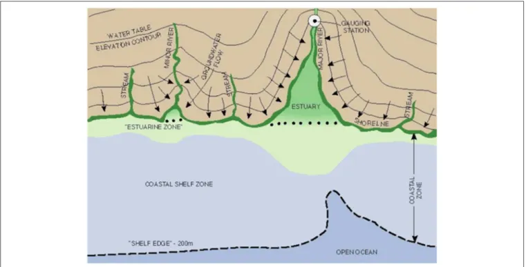
Could groundwater play an important role in such land-sea exchange? Terrestrial groundwater flows down-gradient and ultimately discharges into the sea (Figure 1). This process, part of what is now called “submarine groundwater discharge” (SGD) has become recognized as an important factor in land-sea exchange. While the presence of submarine springs has been known since the days of the Romans, this “invisible pathway” was neglected scientifically for many years because of the difficulty in assessment and the perception that the process was unimportant. This perception has now changed dramatically. Within the last several years there has emerged a recognition that in some cases, groundwater discharge into the sea may be both volumetrically and chemically important. The earlier views were at least partially driven by the difficulty in measuring such flows. Most large rivers are gauged, and their discharges can often be found online. While there is no direct gauge for SGD, techniques have been worked out over the last few decades that allow us to estimate these flows. Here we define SGD as “the flow of water through continental and insular margins from the seabed to the coastal ocean, regardless of fluid composition or driving force” (Burnett et al., 2003). Note that we have added the term “insular” to the original definition. As pointed out before (Zektser and Everett, 2000; Moosdorf et al., 2015) islands typically have higher groundwater discharge fluxes per unit area of land mass than continents. Also note that since we view “groundwater” as any water in the saturated zone of geologic material (Freeze and Cherry, 1979), groundwater is here synonymous with pore water. Importantly, SGD includes waters of any salinity. In fact, fresh water from
FIGURE 1 | Schematic of the coastal zone showing water table contours and terrestrial groundwater flow paths. This illustrates how groundwater flow driven by hydraulic gradients is focused in river valley estuaries and dispersed at highlands. Note that the groundwater contours and flow paths shown control only the terrestrially-driven flow. Marine, geophysical and biological forces contribute substantially to the total flow through coastal sediments. Also note that the gauging station, located well upstream to eliminate tidal effects, will miss all the groundwater discharged below the gauge (Buddemeier, 1996).
recharged aquifers on land only represents a minor portion of the total flux in many cases.Moore (2010)added a “scale length of meters to kilometers” to the earlier definition in order to separate SGD from microscale processes involving pore water exchange. A reasonable idea as the mechanisms driving the flow are very different. See further discussion on this subject in section Geophysical Processes.
Another term that has become widely used in the field is the “subterranean estuary” (STE;Moore, 1999). Basically, the STE is seen as the mixing zone between groundwater and seawater within a coastal aquifer. Within this zone, reactions occur that can substantially modify the composition of these fluids. So, while one might envision the penetration of seawater and its subsequent discharge back into the sea as “seawater recycling,” the geochemical processes within the subterranean estuary may have distinctly altered the composition of the discharging water.
Since there have been a few previous reviews (e.g.,Burnett et al., 2003; Moore, 2010) of SGD research, we will limit this overview to updates and refinements since about 2010. We will restrict our coverage to marine settings including the coastal zone, shelf, estuaries, and lagoons. We will include updates concerning measurements, estimates of SGD magnitudes, geochemical/ecological effects, and cultural/economic aspects. While many SGD studies have been concerned with possible chemical/ecological implications, there have also been recent efforts to evaluate the economic and cultural values associated with SGD (e.g., Michael et al., 2017; Moosdorf and Oehler, 2017; Burnett et al., 2018; Pongkijvorasin et al., 2018). There is
also mounting evidence for the global occurrence of offshore fresh and brackish groundwater reserves underneath continental shelves (Post et al., 2013; Gustafson et al., 2019). Since there is no clear evidence on whether these fossil offshore aquifers are exchanging with the ocean, they are beyond our scope. However, the potential use of these non-renewable reserves as a freshwater resource does provide a clear incentive for future research.
While there was not much scientific work done specifically on SGD prior to the later part of the twentieth century, there were some attempts, many of them related to possible offshore sources of potable water. The lack of interest in the process led Fran Kohout, one of the true pioneers in the field, to comment that “...these marvels of the sea (submarine springs) are justifiably classified as neglected phenomena of coastal hydrology” (Kohout, 1966). He reported in that paper that a literature search only succeeded in finding 15 scientifically-oriented studies concerning SGD. Other early contributions includedLee (1977),
Bokuniewicz (1980), Johannes (1980), and Valiela and D’Elia (1990)among others. These early researchers had the foresight to see that SGD needed increased attention. In their “Preface to a Special Issue” on groundwater discharge in the journal Biogeochemistry,Valiela and D’Elia (1990)commented that “we are very much in the exploratory stage of this field.” We thus see the period before the mid-1990s as the “early days” of SGD research. Things then started to change quickly. In the proceedings of a Land Ocean Interactions in the Coastal Zone (LOICZ) conference dedicated specifically to SGD (“Groundwater Discharge in the Coastal Zone,” Moscow, July 6–10, 1996), it was stated that: “Measurements or estimates of groundwater and associated chemical fluxes, especially over substantial areas or time periods, are notoriously uncertain” (Buddemeier, 1996). Around the same time, some very interesting and provocative data started to appear. Based on large enrichments of226Ra in the shelf waters
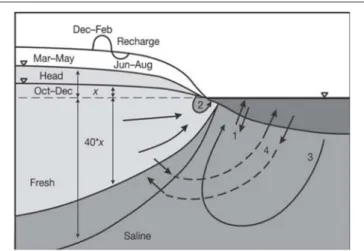
off South Carolina and Georgia,Moore (1996)concluded that the groundwater flux, largely recirculated seawater, to the shelf must be about 40% of the river flux to the same area. A few months later,Cable et al. (1996)reported that radon (222Rn) was significantly enriched in the inner shelf waters of the northeastern Gulf of Mexico. Using a model based on radon inventories they calculated that within a relatively small region (∼620 km2) there was groundwater (combination of saline and fresh) flow in the range of 180–710 m3/s. This is roughly equivalent to the outflow from the Apalachicola River, the largest river in Florida. The value of geochemical tracers quickly became apparent and many studies followed. During this period, which we refer to here as the “developmental period” from the mid-1990s to mid-2000s, there was substantial progress in this field. During this period there were many site studies, considerable advances in technology, more elaborate modeling efforts, and many new insights into driving forces and magnitudes of SGD. Multiple drivers of SGD became recognized (Figure 2). Teams of oceanographers and hydrologists collaborated in meetings and field efforts through sponsorship from the Scientific Committee on Oceanic Research (SCOR), UNESCO and other international agencies (Taniguchi et al., 2002; Burnett et al., 2006). New technologies for measuring geochemical tracers played a key role in getting things moving. For example, Moore and Arnold (1996) developed a
FIGURE 2 | Flow paths and some of the driving forces of SGD. Mechanisms shown include: (1) tidal pumping, (2) nearshore circulation due to tides and waves, (3) saline circulation driven by dispersive entrainment and brackish discharge, and (4) seasonal exchange (Michael et al., 2005).
coincidence counting system that made determinations of223Ra and224Ra much easier and faster. Development of an automated radon-in-water continuous monitoring system greatly simplified radon mapping in the coastal zone (Burnett et al., 2001; Dulaiova et al., 2005). Such technological advances were not limited to geochemical tools. Designs for automated seepage meters based on heat-pulse, dye-dilution, and electromagnetic principles as well as improved electrical resistivity approaches all made substantial contributions (Taniguchi and Fukuo, 1993; Krupa et al., 1998; Paulsen et al., 2001; Sholkovitz et al., 2003; Swarzenski et al., 2006).
Beginning around the mid-2000s, we entered into the “mature stage” of SGD research. SGD investigations have now advanced from hydrogeologic “curiosities” to mainstream science. The scientific community now recognizes that SGD is not only a function of the terrestrial hydraulic gradient but that marine and other drivers result in substantial flow through coastal and shelf permeable sediments. So, while the water table contours shown in Figure 1 may describe the terrestrial flow, the total flow in many cases is dominated by seawater infiltration and subsequent circulation through STEs. As pointed out in more recent reviews, the driving forces of SGD and porewater exchange overlap in both time and space (Moore, 2010; Santos et al., 2012b). There is now widespread recognition that SGD plays an important role in the delivery of nutrients and other dissolved materials to the ocean. While SGD remains somewhat invisible, and still represents a challenge to be measured, it is no longer being overlooked.
GEOPHYSICAL ASPECTS
Geophysical Processes
Literature reviews on the physical drivers of porewater exchange (Huettel and Webster, 2000; Huettel et al., 2014) and SGD (Moore, 2010; Santos et al., 2012b; Robinson et al., 2018) are
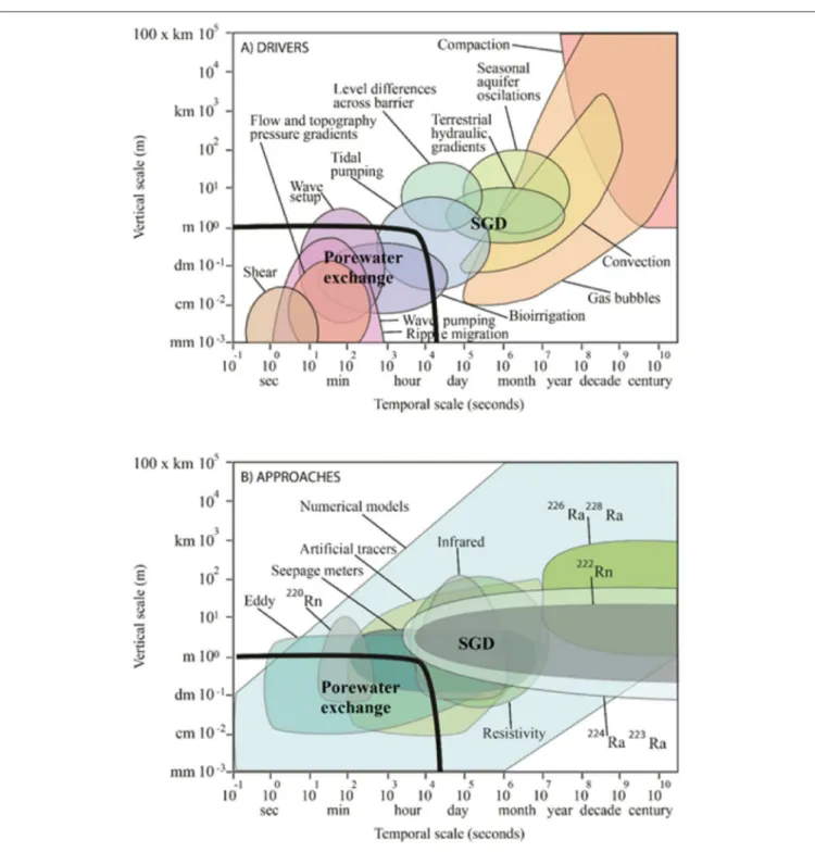
already available. Here, we summarize recent developments in the field and illustrate the challenges of quantifying the multiple overlapping geophysical drivers of fluid flow (Figure 3). SGD and porewater exchange, which we see as different but overlapping processes, are driven by a complex combination of processes occurring over spatial scales ranging from mm
to km, and temporal scales ranging from seconds to years (Santos et al., 2012b). Building onMoore’s (2010)interpretation of SGD, we use length and time scales as boundaries to distinguish the terms porewater exchange and SGD (see thick line in Figure 3). Ours andMoore’s (2010) definition of SGD excludes several small spatial and temporal scale processes such
FIGURE 3 | (A) The operating space of the physical processes driving porewater exchange and SGD in coastal systems. The thick black line separates the porewater exchange space (bottom left) from the SGD space according toMoore (2010)’s definition. (B) The approaches used to quantify SGD (bottom graph) often capture multiple drivers, preventing a straightforward quantification of individual physical processes.
as wave pumping, flow and topographically-induced pressure gradients, and ripple migration that drive advective porewater exchange on scales of <m and <hour. Other important processes such as tidal pumping, wave setup and bio-irrigation may be considered as porewater exchange and/or SGD depending on the context, measurement technique employed, and environmental implication of interest.
Because different techniques tend to quantify overlapping physical processes, confusion when reporting and interpreting results often prevents straightforward comparisons among different field sites and research groups. Most attempts to quantify different drivers of SGD tend to focus on a separation between fresh SGD driven by terrestrial hydraulic gradients vs. saline SGD driven by multiple marine forces. Similar to porewater exchange (<m scale), saline SGD (>m scale) often has large gross yet zero net water fluxes. Earlier investigations relied on salinity observations of water collected from seepage meters to assess the relative contribution of fresh SGD to total SGD (Michael et al., 2003; Santos et al., 2009) as well as a comparison between Darcy’s Law derived fresh SGD vs. total SGD derived from seepage meters (Taniguchi and Iwakawa, 2004) or geochemical tracers (Mulligan and Charette, 2006). More recent investigations have relied on a comparison of salt balance approaches (fresh SGD) vs. geochemical tracers (total SGD). For example, salinity and flow observations were used to infer fresh SGD, while a radium isotope mass balance was used to estimate tidally-driven saline SGD in Australian estuaries (Sadat-Noori et al., 2015, 2017). The different half-lives of radium isotopes have been used to broadly separate SGD from porewater exchange (Tamborski et al., 2017b, 2018).
These investigations provided widespread evidence that the volumetric contribution of fresh SGD is minor compared to saline SGD and porewater exchange at a wide range of field sites. The estimates based on multiple methods also shed light into the physical processes that may be quantified using the different measurement approaches (see overlapping areas in Figures 3A,B). Separating the relative contribution of the different physical processes driving saline SGD is important because longer residence times of seawater within sediments will have a greater impact on the geochemical composition of the exchanging seawater (Seidel et al., 2014; Tamborski et al., 2017a). The multiple time scales of marine driving forces are difficult to quantify using geochemical approaches or field observations. As a result, the roles of currents, tides, waves, and density have been explored mostly using numerical models (Li and Barry, 2000; Robinson et al., 2006; Sawyer et al., 2013).
Tidally-driven SGD has been extensively investigated following the discovery of the beach water table over-height or super-elevation (Nielsen, 1990) followed by the discovery of fresh groundwater tubes underlying upper saline plumes in beach aquifers (Robinson et al., 2006). Seawater infiltrating beaches, fractured aquifers and/or marshes at high tide creates a circulation cell that drives the return of seawater to the ocean at low tide on time scales of days to months (Robinson et al., 2009; Wilson et al., 2015; Geng and Boufadel, 2017; Santos et al., 2019). This process can account for a large fraction of SGD on a local scale, releasing solutes from the beach into the
ocean. The beach water table over-height is driven by faster aquifer recharge during flood tide than discharge at ebb tide, resulting in a localized increase in beach groundwater level that can retard fresh SGD while enhancing saline SGD (Nielsen, 1999; Li et al., 2000). The upper saline plume commonly found in permeable coastal aquifers (Robinson et al., 2018) can alter density-driven seawater circulation since denser seawater overlying fresh groundwater drives convective exchange (Greskowiak, 2014; Röper et al., 2015).
Wave-driven SGD often overlaps the effects of currents and tides (Xin et al., 2010). While waves are known to play a major role in fluid exchange (Sawyer et al., 2013), field investigations have not been able to fully separate their relative contribution to total SGD. Investigations on wave-driven SGD rely on numerical models usually under ideal, phase-averaged conditions (Robinson et al., 2014). Waves expand the tidally-driven upper saline plume in beaches and enhance total SGD (Xin et al., 2010). The importance of waves driving porewater exchange is highly variable with integrated volumetric exchange rates estimated to exceed tidal pumping by one order of magnitude. During storms, wave pumping can increase by orders of magnitude exceeding all other geophysical drivers of fluid flow across the sediment-water interface (Sawyer et al., 2013). In contrast to the effects of tides that occur primarily in intertidal areas, wave-driven porewater and groundwater flow can also occur in shallow subtidal areas.
The overlapping nature of marine drivers of SGD (i.e., currents, tides, waves, density gradients) complicate the individual quantification of the specific physical drivers of SGD. The residence time of seawater circulation cells in coastal aquifers is quite variable ranging from minutes to hours when driven primarily by currents or waves (Anwar et al., 2014), hours to months when driven by tides in intertidal areas (Seidel et al., 2014) and months to thousands of years when driven by density (Post et al., 2013; Seidel et al., 2015; Michael et al., 2016). The multiple driving forces are not necessarily synergistic or additive (Robinson et al., 2018) and interact non-linearly (King, 2012; Xin et al., 2015). For example, while tidal pumping maximizes density-driven convection in intertidal aquifers, it may decrease terrestrial fresh SGD due to the localized elevation of the water table (Robinson et al., 2007). Overlapping tides and waves in numerical models resulted in lower SGD than when either tides or waves are modeled individually (Xin et al., 2010). SGD also responds to past events creating a memory effect that can modify flow for several weeks (Xin et al., 2014). Delayed SGD related to antecedent storms (Smith et al., 2008; Yu et al., 2017), seasonal changes in the terrestrial hydraulic gradient (Michael et al., 2005), and three-dimensional morphological complexities (Zhang et al., 2016) have been described, adding another dimension to the problem and complicating the assessment of the interactions between multiple forces.
Research about the physical drivers of SGD has been developed mostly in permeable sandy aquifer sites. While muddy sediments are often perceived to be impermeable, secondary permeability created by abundant animal burrows can enable advective flow in muddy mangrove and saltmarsh sediments (Xin et al., 2011; Tait et al., 2016). The burrows can connect underlying sandy aquifers containing fresh groundwater to the
surface (Wilson et al., 2015) and enhance tidally-driven saline SGD (Xin et al., 2011; Stieglitz et al., 2013). Groundwater flows in those systems is three dimensional and highly complex due to the patchy nature of burrows, subtle geomorphological gradients, and heterogeneous sediments and vegetation (Moffett et al., 2012; Wilson and Morris, 2012; Xin et al., 2012). Radon and radium observations in multiple mangrove creeks revealed tidally-driven porewater exchange ranging from 2 to 35 cm/day (Tait et al., 2016, 2017). If extrapolated to the global mangrove area, these exchange rates would be enough to filter the entire continental shelf volume in ∼150 years and are equivalent to ∼1/3 of the annual volume of river water entering the oceans (Tait et al., 2016). Because mangrove and saltmarsh porewaters are often highly enriched in carbon and greenhouse gases (Santos et al., 2019), the input of dissolved carbon to the oceans via mangroves may be comparable to the input from global rivers (Chen et al., 2018b). Therefore, muddy mangrove and saltmarsh systems that are widespread on global shorelines deserve additional attention and may disproportionally contribute to SGD and related biogeochemical inputs to the ocean.
High salinity SGD has also been shown in some deltas. For example,Xu et al. (2013, 2014)used radium isotopes to quantify SGD fluxes in the Yellow River Delta. They estimated a SGD flux of 1.3 × 10⁹m3d−1with a range of 2.8 × 10⁸- 3.0 × 10⁹m3d−1.
Even the minimum SGD value was about 3 times higher than the Yellow River discharge at that time. The SGD input of dissolved nutrients was shown to be at least 5 times higher than river input.
Geophysical Methodology
To date, the most commonly applied approaches to quantify SGD fluxes provide estimates over a wide spatial range (Figure 3). A significant gap remains between “embayment-scale” or “beach-scale” geochemical flux estimates on one hand, and seepage meter point measurements on the other. Geophysical methods have been increasingly applied in recent years in order to bridge this gap. The most common geophysical tools applied in SGD studies thus far are based on temperature and salinity variations. In contrast to many geochemical tracer approaches, geophysical approaches can discriminate between freshwater and saline components of SGD (e.g.,Stieglitz et al., 2008a; Tamborski et al., 2015). Particularly applicable to point sources of freshwater SGD, e.g., karstic or volcanic origin, where considerable spatial contrasts in these parameters exist, these approaches provide a “map,” but do not allow for a quantification of SGD fluxes without combining with other methods.
Detection of SGD Sites by Thermal Infrared Sensing Digital thermal infrared cameras are increasingly accessible in price and size, which has resulted in a significant rise in their application over the past decade. By mapping sea surface temperatures with a thermal infrared (TIR) sensor, plumes of buoyant low-density (fresh/brackish) groundwater can be detected. Locations of groundwater discharge are inferred from temperature anomalies (either low or high), based on the seasonal contrast between groundwater and ocean temperature (e.g.,
Varma et al., 2010). Often, TIR observations are used as a guide to target subsequent sampling by quantitative methods (e.g.,
Mulligan and Charette, 2006; Röper et al., 2014). On large spatial scales (km-scale), readily available space borne remote sensing TIR data can be used to identify large SGD inflows sustaining persistent temperature plumes, e.g., in Geographe Bay, Western Australia (Varma et al., 2010), in Java, Indonesia (Oehler et al., 2018), and along the Irish coast (Wilson and Rocha, 2012). TIR cameras are most often mounted on light aircraft (Duarte et al., 2006; Johnson et al., 2008; Lee et al., 2016a; Bejannin et al., 2017) and more recently on drones (e.g.,Lee et al., 2016b) with a typical temperature resolution of 0.1◦
C at a spatial resolution down to 0.5 m (e.g.,Johnson et al., 2008; Kelly et al., 2013). An often-overlooked application is the simple handheld use of an infrared camera, which for instance allows the rapid identification of cm-scale groundwater springs at low tide in the intertidal zone (Röper et al., 2014). Some studies suggest that the surface area of a sea surface temperature plume can be used to quantify SGD fluxes (e.g.,Kelly et al., 2013; Tamborski et al., 2015). This is based on the assumption that the 3D structure of the plume is known or can be estimated. However,Lee et al. (2016a)illustrate the often non-consistent shape of SGD plumes by multiple aerial surveys over a range of seasons and tidal stages. This inherent limitation of surface remote sensing approaches in oceanography is well-documented (e.g., river plumes,Burrage et al., 2003). While there are inherent limitations in using the non-conservative tracer heat/temperature for SGD studies (SGD is not the only “source” of temperature anomalies), this approach has today become a popular part of the SGD toolkit owing to the availability of affordable sensors. Multispectral and hyperspectral sensors are becoming increasingly accessible and may see wider application in the near future. For example, mapping of turbidity plumes caused by sediment remobilization due to groundwater inflow (Kolokoussis et al., 2011). Sea surface salinity would also be an ideal parameter to map and quantify freshwater inflow, but available operational satellite products (SMOS) to date do not have the appropriate resolution for nearshore processes, and airborne low-frequency microwave radiometer sensors remain rare (e.g.,Burrage et al., 2003).
Mapping the Subterranean Estuary With Electrical Ground Conductivity
Early studies of SGD often provided diverse results between “downscaled” geochemical flux estimates and “upscaled” point measurements as, for example, obtained by seepage meters. This is particularly the case where flow patterns are affected by natural or artificial preferential flow paths. While this scale gap remains, it has been significantly reduced over the past decade thanks to advances in a range of additions to the SGD toolkit, including geoelectric methods. When referring to “geoelectric methods,” the terms bulk/ground (electrical) ground conductivity, resistivity (the inverse of conductivity), and electrical tomography are used in the literature. They all refer to basically the same approach, albeit using slightly different instrumentation. The electrical conductivity (resistivity) of coastal sediments is a function of the soil porosity (or pore water fraction) and of the salinity (and temperature) of the interstitial water. In SGD studies, spatial variations of pore water salinity close to the fresh-salt interface are significantly
greater than those of porosity. Geoelectric instrumentation consist of an array of multiple electrodes (minimum four), either directly inserted into the ground (e.g., Stieglitz et al., 2008a), deployed on the sediment surface (e.g., Breier et al., 2005; Swarzenski et al., 2006) or, in some cases, towed behind a boat (Manheim et al., 2004; Su et al., 2014). The geometry of the electrode array determines the volume of sediment over which conductivity/resistivity will be averaged (e.g., Stieglitz et al., 2008b; Henderson et al., 2009).
Geoelectric mapping helps to improve SGD field studies by, for example, informing a more representative placement of seepage meters where preferential flow paths persist (Stieglitz et al., 2007, 2008b). It allows upscaling of point measurements to beach-scale fluxes (Stieglitz et al., 2008a), and repeated measurements along the same transects document the temporal variability of the fresh-salt interface and of fresh groundwater and seawater recirculation fluxes (Taniguchi et al., 2008; Bighash and Murgulet, 2015). They can also be used for the establishment of a sub-surface salt balance model from which SGD fluxes can be calculated (Dimova et al., 2011; Bighash and Murgulet, 2015).
Surface-deployed electrodes and an inversion calculation can be used to obtain a 2D resistivity section with a vertical penetration about one order of magnitude less than the horizontal extension of the array (e.g., 10 m depth along a 100 m transect), at a spatial resolution on the order of a few meters. Using this approach, Taniguchi et al. (2006)
demonstrated that freshwater SGD rates were highest just landward of the saltwater-freshwater interface on a beach in Japan. Gilfedder et al. (2015) showed that a considerable increase in groundwater flux followed storm events on an Australian coastal wetland. Geoelectrical methods are particularly useful to document the temporal dynamics of SGD fluxes and the freshwater-saltwater interface in the subterranean estuary. For example, resistivity mapping on Ubatuba beach (Brazil) showed that the freshwater–saltwater interface moved offshore during a rising tide, in the opposite direction as would be expected, indicating that preferential flow in the fractured rock aquifer was a more important driver of SGD flux than tidal water level fluctuations at this site (Taniguchi et al., 2008).
While interpretation of in situ profile data is straight-forward, uncertainties in both data acquisition (e.g., survey geometry, land topography) and processing (e.g., inversion artifacts, choice of interpolation method) can produce suboptimal results in resistivity inversion calculations of surface arrays (Henderson et al., 2009). These errors can be addressed to some degree by careful ground-truthing (including vertical direct profiling and borehole data) and fine-tuning of the model inversions to the specific characteristics of a field site including sediment type and distribution (Henderson et al., 2009; Johnson et al., 2015). The coupling of geoelectric data and hydrogeological density-driven flow modeling will likely be used more extensively in the future to improve our understanding of the complex and dynamic mixing processes between fresh and saline groundwaters at their interface (Robinson et al., 2006).
Seafloor Mapping and Sub-bottom (seismic) Profiling Similar to other forms of subsurface fluid flow, SGD can affect seafloor morphology. Acoustic seafloor mapping tools (multibeam echosounders and sidescan sonar) providing high resolution maps of the seafloor have revealed the locations of seafloor structures associated with SGD, e.g., “Wonky Holes” (Stieglitz, unpublished data). These seafloor depressions have a diameter of 10 to 30 m and a depth of up to 4 m below surrounding water depths of around 20 m. These features lie some 10 km offshore from the Great Barrier Reef coastline (Stieglitz and Ridd, 2000; Stieglitz, 2005). Schlüter et al. (2004) and Rousakis et al. (2014) mapped pockmarks in the Baltic and Mediterranean Sea, resulting from the interaction between sediment fluidization and bottom currents and sub-aqueous limestone formation (karstification). The investigation of subsurface geological structures by seismic profiling can be instructive to determine the geological origin of SGD and its flow paths (Evans and Lizarralde, 2003; Viso et al., 2010). For example, seismic profiling data suggests that submarine paleochannels, infilled with permeable sediments and capped with impermeable material provide a hydrological connection of coastal aquifers with offshore discharge sites. Thus, providing preferential flow paths for SGD as interpreted from observations along the Great Barrier Reef (Stieglitz and Ridd, 2000; Stieglitz, 2005) and offshore at Wrightsville Beach, USA (Mulligan et al., 2007). In some cases SGD appears to be controlled by fault lines or fracture patterns (Bokuniewicz et al., 2008). A few examples of results from these approaches are shown in Figure 4.
GEOCHEMICAL ASPECTS
Geochemical Processes
The discharge of meteoric groundwater and salty groundwater generally show distinctively different geochemical characteristics. The direct discharge of meteoric groundwater may reflect geochemical characteristics of fresh groundwater, which depend on local hydrogeologic conditions and anthropogenic perturbations. In contrast, the discharge of salty groundwater, which may be composed exclusively of recirculated seawater or a composite of meteoric groundwater and seawater, goes through vigorous biogeochemical alterations in the subterranean estuary (STE) (Santos et al., 2008).
Geochemical processes in the STE are very different from those observed in river estuaries in many respects. The most distinct difference is the fact that the ratio of solid to liquid in a STE is much higher than that in river estuaries. Therefore, reactive elements can be more easily removed, and pH may be enhanced due to the adsorption of H+ on oxide surfaces in an organic-poor STE (Lee and Kim, 2015) or reduced due to production of CO2 during organic matter respiration
(Cyronak et al., 2014). In an organic-rich STE, various re-mineralized components of organic matter, including nutrients, dissolved organic carbon (DOC), dissolved inorganic carbon (DIC), fluorescent dissolved organic matter, and trace elements, are highly enriched and pH is generally lower. The temperature of groundwater is relatively constant compared with surface waters, especially in temperate regions. In addition, STE waters are often
FIGURE 4 | (Top) Airborne Infrared maps from beaches on Long Island (USA) elucidating cold SGD plumes (adapted fromTamborski et al., 2015); (Center) bulk ground conductivity transect indicating preferential freshwater SGD flow path. Arrow length indicates SGD flow rates measured with seepage meters at the respective locations (adapted fromStieglitz et al., 2008a); (Bottom) Sub-bottom (seismic) profile of a riverine paleochannel and associated Wonky Holes (Great Barrier Reef, Australia) (Stieglitz, unpublished data).
enriched in reduced species [NH+
4, Fe(II), etc.]. Therefore, the
STE has been found to be much more dynamic in terms of biogeochemical alterations, relative to river estuaries.
Amongst chemical species, the fluxes of nutrients via SGD have been studied most extensively since they have significant impacts on marine ecosystems. In a STE, the behavior of N species is very complicated depending on the redox conditions and organic matter re-mineralization. NH+4 is often found to be
removed by nitrification in oxic conditions (Spiteri et al., 2008; Anwar et al., 2014; Anschutz et al., 2016) or also by adsorption onto particles (Buss et al., 2004; Lorah et al., 2009). Under anoxic conditions, dissolved N can also be removed by forming gaseous species (Kroeger and Charette, 2008; Couturier et al., 2017). Si and P in groundwater can be removed in STE by adsorption, but P can be potentially desorbed from the sediment surface layer under much higher Si concentrations since they compete for the same specific ligand sites including Fe- and Mn-, and Al-oxides (Cho et al., 2019b). However, in organic-rich STEs, all these nutrients are highly enriched by re-mineralization. Recent studies also documented the importance of dissolved organic nitrogen (DON) and phosphorus (DOP) in delivering nutrients through SGD (Kim et al., 2013; Sadat-Noori et al., 2016; Stewart et al., 2018). Therefore, we can conclude that the impact of SGD is very different depending upon the hydrogeological and biogeochemical conditions of the STE.
There have been many upscaling attempts to gauge the magnitude of nutrients fluxes through SGD on basin scales. SGD-driven fluxes of nutrients are generally significant in coastal waters (Kim et al., 2005; Rodellas et al., 2015a; Cho et al., 2018). Recently the global volume of fresh submarine groundwater discharge (FSGD) has been estimated around 1% of river discharge (Luijendijk et al., 2019; Zhou et al., 2019), less than the previously estimated 5–10% (Oki and Kanae, 2006). Consequently, the global fluxes FSGD of DIN, DIP, and DSi through FSGD to the global ocean seem to be below 10% of those from river discharge (Cho et al., 2018and references therein). However,Cho et al. (2018)showed that the fluxes of DIN, DIP, DSi through total (fresh+saline) groundwater discharge on a global scale were comparable to river inputs. Rahman et al. (2019)also showed a similar result for DSi input via saline SGD, accounting for a 25–30% increase in global estimates of net DSi inputs (riverine, SGD, aeolian, hydrothermal, and seafloor weathering) to the ocean.
SGD may also play an important role for the fluxes of terrestrial carbon to the ocean as a form of DOC or DIC. In addition, a significant amount of marine carbon is also returned back to the ocean by SGD. In general, marine vs. terrestrial sources of DOC and DIC are differentiated by stable carbon isotopes (Gramling et al., 2003). In a STE, DOC is transformed to DIC via microbial processes. DOC and DIC are also formed within a STE by the bacterial degradation of particulate organic carbon (POC). Therefore, many STEs show higher DOC concentrations in groundwater than coastal seawater, indicating that SGD is a potential DOC source to the near-shore ocean (Webb et al., 2019). However, the contribution of SGD to the marine DOC budget remains unknown relative to other sources such as in-situ production of DOC in the
euphotic zone. Clearly, the importance of SGD on the fluxes of refractory and aged DOC to the ocean should be more extensively evaluated in the future.
Fluxes of DIC were found to be important in many oceanic regions. By considering SGD in the DIC budget in the ocean, the sink or source regions of CO2 have been re-evaluated (Cai et al., 2003; Dorsett et al., 2011; Liu et al., 2012). The importance of SGD-derived DIC fluxes to the oceans have been particularly emphasized in carbon-rich mangrove forest areas (Chen et al., 2018b) and have been suggested to exceed regional river inputs in Florida (Liu et al., 2012) and in an Australian embayment (Stewart et al., 2015). In addition, DIC concentrations in STEs and their associated contributions to the ocean showed large seasonal variations (Wang et al., 2015). Fluorescent DOM (FDOM), especially humic-like varieties, is generally enriched in STEs, and thus SGD showed a significant influence on the coastal budget of humic-like FDOM (Kim et al., 2013; Suryaputra et al., 2015). Kim and Kim (2017) documented that fresh groundwater in Jeju Island, Korea, generally showed lower DOC due to degradation and higher humic-like FDOM produced from bacterial degradation of labile DOC and POC in aquifers. They suggested that SGD provides an environmental condition favorable for coral ecosystems by reducing UV penetration and DOC concentrations. Therefore, SGD-associated carbon studies should be conducted not only for establishing local/regional carbon budgets but also for understanding marine ecosystem changes and implications for ocean acidification.
Studies of trace element fluxes associated with SGD have shown that many elements exhibit non-conservative behavior within a STE. Although river estuaries are generally sinks of trace elements due to flocculation of particle reactive elements, STEs often display significantly higher trace element concentrations relative to river water or seawater in association with re-mineralization of organic matter, release from oxides, and desorption from sediments (Charette and Sholkovitz, 2006; Santos-Echeandia et al., 2009). Therefore, the behavior of trace elements in STEs is largely dependent on pH, Fe/Mn oxides, and bacterial activities. Due to such a reactive nature of trace elements to particles, colloids play an important role in the delivery of trace elements from STEs to the coastal ocean (Kim and Kim, 2015). In Jeju Island, Korea,Jeong et al. (2012)showed that the change (∼20-fold) in concentrations of trace elements (i.e., Al, Mn, Fe, Co, Ni, and Cu) in the STE resulted in the matching change in inventory of these elements in coastal waters. Although a STE can serve as a significant source for most trace elements which are extremely low in seawater, STEs can be an important sink of conservative elements in seawater by changing redox conditions. For example, forming reduced conditions for U uptake (Charette and Sholkovitz, 2006) and precipitation of Mn oxides for Mo adsorption (Beck et al., 2010). Although a few local or regional studies demonstrated the importance of SGD for the delivery of trace elements to the ocean (Moore, 2010; Jeong et al., 2012; Kim and Kim, 2015; Trezzi et al., 2016), so far the global or basin scale importance is largely unknown. It is particularly important for Fe since the growth of marine planktons could be limited by extremely low-level Fe in seawater, although it is a major element in the earth’s crust.
Thus, it is very important to look at the magnitude of SGD-driven dissolved trace elements to the ocean for basin-scale as well as local/regional scales in association with climate and ecosystem changes.
Among trace elements, rare earth elements (REE) associated with SGD have received considerable attention recently. In general, high enrichment of REE, relative to the simple binary mixing of meteoric groundwater and seawater has been observed in STEs, although the STE can also act as a sink for heavy REEs (HREE) owing to adsorption onto Fe oxides (Johannesson et al., 2011). In STEs, light REEs (LREE) are more readily exchangeable on aquifer mineral surfaces than HREEs, and HREEs and middle REEs (MREE) exhibit a greater association with oxide minerals (Willis and Johannesson, 2011; Chevis et al., 2015). Thus, redox conditions along the flow path of groundwater can affect REE concentration and fractionation (Johannesson et al., 2005, 2011; Tang and Johannesson, 2005, 2006). A case study carried out on a sandy STE in Florida (Chevis et al., 2015) showed that advection and bio-irrigation differentially affect REE fluxes to the ocean as fresh groundwater is enriched in HREEs, while marine pore-water is enriched in MREE in association with the reductive dissolution of Fe oxides/oxyhydroxides. Therefore, REE contributions to coastal waters are clearly identified due to large contributions of different REE patterns to coastal waters (Kim and Kim, 2011; Johannesson et al., 2017). Much more extensive studies are necessary to determine SGD’s contribution to the budgets and fractionations of REE on basin and global scales.
The compilation of Nd isotopes in the global ocean showed that the traditionally believed main Nd sources, e.g., rivers and atmosphere, cannot explain the large difference in Nd isotope ratios and concentrations in different basins, the so called “Nd paradox.” Recent studies showed that SGD can account for the missing Nd source (>90% of the known source;Tachikawa et al., 2003; Johannesson and Burdige, 2007; Chevis et al., 2015). However, much more local and regional evidence are necessary to validate this hypothesis. Besides, large enrichments of alkaline earth elements (Sr, Ba, and Ra and their isotopes) have been successfully utilized to trace SGD to the ocean. SGD inputs of Sr, with less radiogenic Sr than seawater, influence the Sr isotope budget in the ocean, making up 13–31% of the marine Sr isotope budget (Beck et al., 2013). This fluvial input is comparable in magnitude to the flux driven by submarine hydrothermal circulation through mid-ocean ridges. Yet, the use of Sr isotopes as an SGD tracer is still challenging since Sr isotopic composition and distribution of the coastal waters are rather complicated (Huang et al., 2011). Such a complicated pattern seems to be associated with different isotopic ratios from different sources, fractionations along the path, and non-conservative behaviors within the STE (Andersson et al., 1994; Xu and Marcantonio, 2004; Huang and You, 2007). Since Ra isotopes are one of the more useful SGD tracers, more details concerning the Ra isotope applications for flux estimations will be covered in the following methodology section.
Geochemical Methodology
Coastal salinity may seem like an obvious SGD tracer but it has interferences from terrestrial surface runoff and it does not capture the recirculated seawater component of SGD. Therefore, since the 1990’s several groundwater tracers have been applied for SGD quantification in addition to, or instead of salinity (Table 1). Among others, these include radium, radon, methane, silica, hydrogen, and oxygen stable isotopes of water (Bugna et al., 1996; Cable et al., 1996; Campbell and Bate, 1996; Moore, 1996; Godoy et al., 2013; Rocha et al., 2016). Radon and radium isotopes have been applied most frequently, with 40% of the published 473 SGD articles between 2015 and 2019 applying one or both (Web of Science, 2019). The advantage of radon (222Rn, T1/2 = 3.8 days) is that automated measurement methods allow for easy time-series and spatial survey measurements. Due to the large concentration gradient between groundwater and ocean water, its gaseous nature, and relatively short half-life, radon is applicable for assessment of recent and local SGD inputs. Radium analysis of seawater, on the other hand, requires a collection of large volume samples and laboratory or shipboard measurements. However, its great advantage is that radium has four isotopes with half-lives covering a wide range of time scales (224Ra, T1/2
=3.6 days; 223Ra, T1/2 = 11.4 days; 228Ra, T1/2 = 5.7 years; and226Ra, T1/2 =1,600 years) thus allowing SGD assessment on multiple spatial and temporal scales. In addition, radium isotopes can be used to estimate water mixing and residence times (Charette et al., 2008). For example, beyond the embayment scale, ocean-basin scale SGD estimates were recently performed using inventories of the relatively long-lived228Ra (Kwon et al., 2014). Uncertainties are often high for both radon and radium mass balance estimates, largely but not exclusively, because of the difficulty in constraining a value for the groundwater “end-member” (the concentration of the tracer in the discharging groundwater;Burnett et al., 2007; Schubert et al., 2019).
SGD tracer measurement methods have recently been improved to enhance detection limits and make more efficient measurements over longer time periods as well as obtaining finer spatial scale applications. One example of improvement for radium measurements is a large-volume (over 1,500 L/4 h) sampling method using commercially available in situ pumps modified to accept MnO2 coated filter cartridges (Henderson et al., 2013). The method has been applied on continental shelves as well as in open ocean environments and is a promising tool to significantly increase the number of observations of ocean basin-scale radium isotope inventories in the coming years. Improvement in the existing coastal radon detection methods via a commercially available radon-in-air detectors (RAD7, Durridge) was achieved by more efficient gas stripping via improved air-gas exchanger design (Santos et al., 2012a) and use of membrane extractors (Gilfedder et al., 2015). These allow for more powerful and efficient pumping and better radon measurement response rates during coastal surveys. The latter issue was also tackled byPetermann and Schubert (2015), who introduced a methodology to correct radon data collected using an air-water exchanger (RAD-Aqua, Durridge) connected to a RAD-7 radon detector for its response delay when moving
TABLE 1 | Summary of the main geochemical tracers used in SGD related studies.
Tracer Measurement Lab/in situ Application References Salinity Conductivity In situ Fresh water SGD
226Ra Gamma-spec Lab SGD estimation Moore, 1996 222Rn Lucas cells (alpha-scintillation) Lab SGD estimation Cable et al., 1996 222Rn Automated (RAD-7, alpha-spectrometry) In situ SGD estimation
-temporal -spatial
Burnett et al., 2001; Dulaiova et al., 2005
222Rn Underwater gamma-spec (HPGe & NaI) In situ SGD estimation
-temporal -spatial
Povinec et al., 2006; Tsabaris et al., 2012; Dulai et al., 2016
222Rn Automated (RAD-7, alpha-spectrometry) Lab, in situ STE residence time
estimation
Goodridge and Melack, 2014; Oh and Kim, 2016
220Rn Automated (RAD-7, alpha-spectrometry) In situ SGD prospecting
SGD estimation -temporal -spatial
Chanyotha et al., 2014, 2018; Swarzenski et al., 2016 Methane Gas chromatography Lab SGD estimation Bugna et al., 1996 Methane METS membrane diffusion detector TETHYS in-situ
underwater mass spectrometry
In situ SGD estimation -temporal -spatial
Kim and Hwang, 2002; Dulaiova et al., 2010
224Ra,223Ra RaDeCC (alpha-scintillation) Lab Water mass mixing,
residence times, SGD estimation
Moore and Arnold, 1996; Charette et al., 2008
224Ra/228Th RaDeCC (alpha-scintillation) Lab Porewater exchange Cai et al., 2014 224Ra,223Ra RaDeCC (alpha-scintillation) Lab Porewater exchange Rodellas et al., 2015b 228Ra Gamma-spectrometry Lab Ocean basin scale SGD Moore et al., 2008;
Kwon et al., 2014
226Ra,228Ra Large volume pump + gamma spectrometry Lab Ocean basin scale SGD Henderson et al., 2013 224Ra,228Ra Underwater gamma-spectrometry In situ Residence times, SGD
estimation
Eleftheriou et al., 2017
fDOM, humification index Fluorometry Lab SGD estimation Nelson et al., 2015 Silica Colorimetry Lab SGD estimation Street et al., 2008 δ18O and δ2H Optical spectroscopy Lab SGD estimation Godoy et al., 2013;
Rocha et al., 2016
between high and low radon activity water masses. Schubert et al. (2019) recently suggested additional improvements in the application of radon mass balance approaches that should improve corrections for radon losses from mixing and atmospheric evasion.
Since the “early days” of SGD studies, there has been a natural progression in improving radon measurement methodologies from labor-intensive grab samples collected in the field and analyzed in the lab or on ships (Mathieu et al., 1988), to the use of automated systems such as the RAD-AQUA (Burnett et al., 2001), to completely automated detection systems that can work unattended for months to years. Examples of the latter approach include autonomous water-proofed gamma-spectrometry systems that are passive and do not require power-demanding water pumping (Tsabaris et al., 2012). A mobile underwater in-situ gamma-ray spectroscopy system was successfully applied for coastal surveys of radon and 224Ra as a ship-deployed tow system (Patritis et al., 2018) and was also developed for long-term deployment on a permanently moored station where it recorded hourly radon measurements for multiple years (Dulai et al., 2016 and see Figure 5). These
novel technologies bring the ability to perform longer and higher resolution SGD monitoring in diverse field settings, which will help document trends in SGD in different hydrogeologic and climatic settings, under extreme weather events, excessive groundwater pumping trends, and sea level rise scenarios. Eventually, such systems could be deployed as a global network.
There have been several new SGD tracers introduced recently. Another isotope of radon,220Rn, also called “thoron,” has been
used for SGD prospecting, i.e., finding points of discharge as one must be close to a source to detect this very short-lived isotope. In an effort to employ220Rn as a groundwater tracer,Huxol et al. (2012)showed that while220Rn is easily detected in soil gas, it is often undetectable in groundwater. This is the case because under saturated conditions, migration of thoron through water is so slow that radioactive decay reduces the concentration to undetectable levels. However, flowing water apparently disturbs the immobile water layers stimulating the transfer of220Rn to the flowing water phase (Huxol et al., 2013). Thus, while thoron is difficult to detect in groundwater, it does serve as a good groundwater discharge tracer. Chanyotha et al. (2014) found intermittent thoron spikes in a 25-km stretch of a Bangkok canal
FIGURE 5 | (A) An autonomous gamma-spectrometer [NaI(Tl)] was deployed off the coast of Kiholo Bay, HI, USA. (B) Gamma-ray spectra were collected in the surface waters at hourly resolution. (C) The spectra during low tide show radon decay products, while at high tide radon and its progenies are diluted to below detection levels. (D) Hourly radon measurements over multiple years (a 9-month record shown here) allows us to evaluate SGD dynamics over tidal and seasonal time scales. Data fromDulai et al. (2016).
at essentially the same locations in surveys run along the same line 4 years apart. They also introduced a tool, the “meaningful thoron threshold,” that ensures that a positive reading at or above the threshold has a 90% certainty of being a real detect. Thoron was also used in coastal spring discharge monitoring in Hawaii (Swarzenski et al., 2016).
Another natural SGD tracer involves dissolved organic matter (DOM). For example, SGD is often enriched in humic-like fluorescent DOM (Kim and Kim, 2017) and Nelson et al. (2015)demonstrated the utility of using indices of humidification derived from DOM in discharging groundwater as a tracer of SGD dispersal in nearshore waters.
There is renewed interest in the application of other U/Th series radionuclides, for example the224Ra/228Th disequilibrium pair to study SGD and pore-water exchange dynamics (Cai et al., 2014). It has been demonstrated that carefully constructed radon and radium isotope mass-balances with well-defined
end-members allow the quantification of and distinction between large-scale SGD and small-scale pore water exchange (Rodellas et al., 2015b; Cook et al., 2018). On a larger-scale form of exchange, radon has been applied to estimate beach pore water residence times and the flushing of a subterranean estuary, which showed positive correlation with tidal amplitudes and associated nutrient and dissolved organic carbon enrichment (Goodridge and Melack, 2014) and strong correlation with seawater intrusion (Oh and Kim, 2016). Radium and radon have also been combined with and used to document SGD-derived greenhouse gas fluxes in for example, a subtropical estuary (Sadat-Noori et al., 2016), the Amazon region (Call et al., 2019), and the Arctic (Lecher et al., 2015).
While geochemical tracers continue to provide valuable information for SGD studies, the most notable trend in the field is the application of multiple techniques that include geochemical tracers, geophysical approaches, direct
FIGURE 6 | Biological production in coastal ecosystems based on nutrients supplied through SGD. The numbers refer to the driving forces identified in Figure 2.
measurements, and hydrological modeling (e.g.,Taniguchi et al., 2015). Such applications using multiple approaches decrease the degrees of freedom when interpreting SGD processes in often complex environments.
BIO-ECOLOGICAL IMPACTS
Bio-ecological Processes
Groundwater discharge has been recognized as a mechanism for transporting land-derived materials to the sea. Nutrients, carbon, metals, and other materials, which are dissolved in terrestrial groundwater, can drive bio-ecological processes in coastal seas. These effects are enhanced by recirculated seawater as it reacts within the aquifer sediment (see the Geochemical section). SGD can also act as a conduit of anthropogenic pollutants to coastal regions, and the lower salinity and pH associated with some types of SGD can stress local marine biota (reviewed in Lecher and Mackey, 2018).
Most studies of marine biota with respect to SGD focus on primary producers, because they provide the base of marine ecosystems as well as the chief response to nutrient supply via SGD (Figure 6). To date, many studies have revealed that nutrients transported through groundwater can support benthic and water column primary production in various coastal ecosystems. For example, SGD drives benthic primary production in the intertidal zone of the Yellow Sea (Waska and Kim, 2010, 2011). SGD also contributes significantly to reef productivity and/or calcification (Kamermans et al., 2002; Greenwood et al., 2013; McMahon and Santos, 2017). In a coastal water column, phytoplankton community structure was shown to be altered by SGD (Troccoli-Ghinaglia et al., 2010; Blanco et al., 2011; Adolf et al., 2019). More recently, a direct relationship between SGD and in situ phytoplankton primary productivity in nearshore coastal areas in Japan was found (Sugimoto et al., 2017). In Mediterranean coastal lagoons,Andrisoa et al. (2019)
provided direct evidence for the role of karstic groundwater and porewater fluxes in sustaining primary production. Nutrient addition bioassay experiments support the view that SGD acts as a continual nutrient source (Gobler and Boneillo, 2003; Lecher et al., 2015).
Conversely, excess nutrient loadings via polluted groundwater into coastal seas may cause cultural eutrophication and microalgal blooms. In South Korea, SGD was identified as the most likely nutrient source triggering harmful algal blooms (HABs) and green tides (Hwang et al., 2005; Lee et al., 2009; Kwon et al., 2017; Cho et al., 2019a). In oligotrophic coastal reef environments, significant effects of SGD on marine biota were reported with their magnitudes varying according to land-use practices. The effects were shown to be most intense in locations with high anthropogenic impacts (Amato et al., 2016, 2018). Macroalgal overgrowths of coral reefs worldwide has been associated with nutrient inputs from SGD (Knee and Paytan, 2011). On the other hand, reef structure can also impact the nutrient load discharged into the sea by SGD (Oehler et al., 2019). In the case of benthic communities, most SGD linkages are reported from intertidal regions. Several patterns have emerged from a limited number of studies suggesting that intertidal fresh SGD can change microbiological communities (Adyasari et al., 2019), determine species diversity, distribution, biomass distribution, and proliferation of benthic animals (e.g.,Ouisse et al., 2011; Leitão et al., 2015; Foley, 2018). For example, benthic communities in the vicinity of freshwater SGD are often characterized by reduced species richness and diversity, due to high abundances of a small number of euryhaline/freshwater-tolerant species (Zipperle and Reise, 2005; Dale and Miller, 2008). Intertidal SGD has been associated with a shift in dominant species of macrofauna and meiofauna and can exclude ubiquitous species that are in the surrounding marine environment (Zipperle and Reise, 2005; Welti et al., 2015; Shoji and Tominaga, 2018). SGD might also moderate pore-water
temperatures and provide a refuge in sediment for macrofauna against extreme temperatures (Miller and Ullman, 2004). Overall, intertidal SGD may enhance biodiversity and species richness on a broader spatial scale.
SGD has been believed to contribute to coastal fisheries production including extensive aquaculture (e.g., oyster and mussel) in many locations around the world (Moosdorf and Oehler, 2017; Chen et al., 2018a; Shoji and Tominaga, 2018). Although there was little scientific evidence until recently, a growing body of interdisciplinary work is now demonstrating an ecological linkage between SGD and fisheries resources. For example, the Mediterranean mussel is a highly valuable commercial species. At the Olhos de Aqua beach in Portugal, groundwater inputs were recognized as increasing abundance and body size of these mussels (Piló et al., 2018). Cage experiments of the mussel Mytilus galloprovincialis in Salses-Leucate lagoon in France revealed that groundwater discharge provides favorable environmental conditions (i.e., higher temperature and food availability) for faster growth (Andrisoa et al., submitted). This is thought to be the case as groundwater discharge is a major source of nutrients and affects primary production within these ecosystems (Rodellas et al., 2015a; Andrisoa et al., 2019). Along the volcanic coast of northern Japan, fresh groundwater is an important factor providing suitable environment for phytoplankton that drives the high quality of the sessile bivalve Crasslstrea nippona, a commercially important local oyster (Hosono et al., 2012). In the Caribbean region, a groundwater-fed inlet provides a habitat for queen conch Lobatus gigas populations, which is one of the most important fishery resources in the region (Stieglitz and Dujon, 2017).
An increase of fish abundance and biomass and utilization of nursery areas has been observed in the vicinity of SGD (Hata et al., 2016; Utsunomiya et al., 2017; Starke et al., submitted;
Yamane et al., 2019). The first location where an impact of SGD on fish abundance was directly recorded was in Obama Bay, Japan (Utsunomiya et al., 2017). There, the effect of nutrients transported via SGD on the food-chain was highlighted, because primary production was shown to be higher near SGD sites (Sugimoto et al., 2017). Furthermore, in the tidal flat of Seto Inland Sea, Japan, abundant juveniles of the marbles sole Pseudopleuronectes yokohamae were found near SGD sites with abundant prey organisms (Hata et al., 2016). Experimental evidence confirmed that the juvenile P. yokohamae obtained elevated levels of nutrition in the vicinity of SGD (Fujita et al., 2019). These findings demonstrated that SGD-derived nutrients enhanced marine fish production.
SGD has been shown to influence marine biota across a variety of coastal ecosystems. However, the mechanisms by which SGD affects primary production as well as marine animals differ from one ecosystem to another depending upon the hydrogeographical properties such as type of groundwater discharge (i.e., spring or seepage), location, species present, nutrient content of the groundwater, SGD flux, among other factors (Sugimoto et al., 2017; Shoji and Tominaga, 2018). Additional research is needed for a comprehensive assessment of SGD’s impact on marine ecosystems.
Bio-ecological Methodology
Four-decades after Johannes’s benchmark paper (Johannes, 1980), several SGD studies confirmed that groundwater is a significant source of nutrients to coastal seas. Although there is no doubt that SGD-derived nutrients contribute to marine organisms and ecosystem functions, evidence of the actual linkage between SGD and marine organisms is limited. Evidence seems best at some specific geological sites (e.g., karstic and volcanic regions) and intertidal sandflats where the discharge of groundwater can be directly viewed (Moosdorf and Oehler, 2017; Lecher and Mackey, 2018). In some cases, gas bubbles and excessive phenomena such as eutrophication and algal blooms are tied to SGD (Knee and Paytan, 2011). The difficulty in making the SGD-ecological linkage may be explained in two ways. First, marine organisms (i.e., microalgae, macroalgae, and animals) living in coastal waters or sediments are subject to various physical and biogeochemical processes that can affect their growth and physiology. In addition, nutrients supplied from multiple sources including rivers, atmospheric deposition, oceanic waters, and organic matter regeneration as well as groundwater inputs complicate an SGD assessment. Second, the pathway of SGD is invisible restricting our investigations in most coastal ecosystems. However, technological advances over the last decade have increased our ability to assess the ecological linkage to SGD in systems from local to shelf scales.Lecher and Mackey (2018)synthesized the effects of SGD on marine biota. Here we focus on how to assess the impact of SGD on marine organisms and ecosystems based on the latest methodological advances (Table 2).
Stable nitrogen isotope ratios (δ15N) of primary producers are well-known to be useful in detecting the direct linkage between groundwater inputs and marine organisms when the dissolved inorganic nitrogen (DIN) of groundwater is isotopically distinct from other DIN sources. For example,McClelland and Valiela (1998)demonstrated a strong relationship between increases of δ15N of NO−
3 in groundwater and increases in δ15N of various
primary producers in several estuaries in Massachusetts. A clear positive relationship between seagrass δ15N and the estimated
groundwater flux was a pioneering work for this approach (Kamermans et al., 2002). To date, several studies have traced the behavior and fate of groundwater DIN using the δ15N of primary producers, seagrasses, and macroalgae from local to regional scales (e.g., Lapointe et al., 2004, 2015; Derse et al., 2007; Honda et al., 2018; Andrisoa et al., 2019). In comparison to phytoplankton, macroalgae and seagrasses provide a time-integrated view of the N sources. Given that macroalgae directly take up nutrients only from the water column whereas seagrass does so mainly from interstitial waters, macroalgae is considered the more appropriate tool to assess the long-term availability of nitrogen in the overlying water column (Umezawa et al., 2002). In recent studies, researchers have deployed pre-treated macroalgae to assess the time-integrated impacts of SGD on a fine spatial scale. For example,Amato et al. (2016) quantified a groundwater impacted area in Kahului Bay, Hawaii, using the δ15N of both in situ macroalgae collected from intertidal and subtidal zones as well as pre-treated macroalga deployed for a short-term in anchored cages. Similar studies have been
TABLE 2 | Summary of the main bio-ecological parameters used in SGD related studies.
Tracers Measurement Lab/In situ Application References δ15N and δ13C Isotope ratio mass spectrometer (IRMS) Lab Tracing nitrogen and
carbon flows, food web analysis
McClelland and Valiela, 1998; Hata et al., 2016; Andrisoa et al., 2019 δ15N of macroalgae deployed in the water IRMS and macroalgae incubation Lab + in situ Spatial mapping of
SGD impacts on primary producers
Amato et al., 2016
Nutrient Submersible colorimeter In situ High resolution monitoring of nutrient
Blanco et al., 2011
Nutrient Spectrophotometry Lab Primary production estimation
Waska and Kim, 2011; Wang et al., 2018 Chlorophyll Fluorometry Lab, in situ Biomass of
phytoplankton,
Kobayashi et al., 2017; Honda et al., 2018 Photosynthetic pigments High performance liquid chromatography (HPLC) Lab Class differentiation of
benthic algae
Waska and Kim, 2010
Phytoplankton Spectral fluorometry In situ Class differentiation of phytoplankton
Blanco et al., 2011
Phytoplankton Flow cytometer Lab Size differentiation of phytoplankton
Lecher et al., 2015; Adolf et al., 2019 Phytoplankton Bottle incubation with nutrient addition Lab + in situ Growth rate of
phytoplankton, Limiting nutrients
Gobler and Boneillo, 2003; Lecher et al., 2015
Phytoplankton Bottle incubation with enriched DI13C addition Lab + in situ Primary productivity of phytoplankton
Sugimoto et al., 2017
Dissolved oxygen Optical oxygen sensor In situ Net ecosystem production, photosynthesis, respiration
Honda et al., 2018
pCO2 Non-dispersive infrared sensor In situ Net ecosystem production, photosynthesis, respiration
Santos et al., 2012a; Maher et al., 2019
Number of benthic animals Core sampler In situ Biomass and diversity of animals, Habitat use
Dale and Miller, 2008; Leitão et al., 2015 Number of fish Net In situ Biomass and diversity
of animals, Habitat use
Hata et al., 2016; Yamane et al., 2019 Behavior of animals Acoustic telemetry In situ Habitat use Stieglitz and Dujon,
2017 Shell length of bivalve Cage experiment In situ Growth rate (Andrisoa et al.,
submitted) Total length of fish Cage experiment In situ Growth rate Fujita et al., 2019
done at a fringing coral reef ecosystem of Hawai’i Island (Abaya et al., 2018) and four embayments in Tutuila, American Samoa (Shuler et al., 2019).
However, the exact relationship between algae and SGD is sometimes difficult to interpret because the isotopic composition of the source nitrogen is variable and can cause uncertainty when interpreting the isotope fractionation during the assimilation, especially if more than one form of nitrogen is present (e.g., NO−
3 and NH
+
4), or if more than one source of nitrogen is
available (e.g., riverine, groundwater, oceanic, and regenerated nitrogen; Sugimoto et al., 2010, 2014). Thus, the utilization of the δ15N of primary producers as a proxy for the δ15N of nutrient sources is difficult unless adequate information is obtained regarding the δ15N of the various sources. For example, in the Waquoit Bay estuarine system, a comparison
of the δ15N of phytoplankton, NO−3, and NH +
4 revealed that
phytoplankton derived 3–47% of their N from groundwater NO−
3, while the major N source was regenerated NH + 4
(York et al., 2007).
Along with analyses of δ15N, gradients in the stable carbon
isotope ratio (δ13C) between fresh groundwater and marine end members (Gramling et al., 2003) can be utilized to detect the direct linkage between SGD and organisms. For example, the δ13C signature of macrophyte and phytoplankton in coastal lagoons on the French Mediterranean coastline shows the contribution of karstic groundwater discharge and porewater exchange as significant sources of dissolved inorganic carbon to primary production (Andrisoa et al., 2019). Therefore, these δ15N and δ13C signals in primary producers can be traced through some marine food webs. Although there is still no clear evidence,