HAL Id: inria-00465141
https://hal.inria.fr/inria-00465141
Submitted on 1 Nov 2010
HAL is a multi-disciplinary open access
archive for the deposit and dissemination of
sci-entific research documents, whether they are
pub-lished or not. The documents may come from
teaching and research institutions in France or
abroad, or from public or private research centers.
L’archive ouverte pluridisciplinaire HAL, est
destinée au dépôt et à la diffusion de documents
scientifiques de niveau recherche, publiés ou non,
émanant des établissements d’enseignement et de
recherche français ou étrangers, des laboratoires
publics ou privés.
OSIF: A Framework To Instrument, Validate, and
Analyze Simulations
Judicaël Ribault, Olivier Dalle, Denis Conan, Sébastien Leriche
To cite this version:
Judicaël Ribault, Olivier Dalle, Denis Conan, Sébastien Leriche. OSIF: A Framework To Instrument,
Validate, and Analyze Simulations. SIMUTools2010, Mar 2010, Torremolinos, Spain. �inria-00465141�
OSIF: A Framework To Instrument, Validate, and Analyze
Simulations.
Judicaël Ribault - Olivier Dalle
INRIA - CRISAM
University of Nice Sophia Antipolis I3S-UMR CNRS 6070
BP93 - 06903 Sophia Antipolis, France
[email protected]
Denis Conan - Sebastien Leriche
Institut Télécom, Télécom SudParis UMR CNRS SAMOVAR
9 rue Charles Fourier 91011 Évry, France
[email protected]
ABSTRACT
In most existing simulators, the outputs of a simulation run consist either in a simulation report generated at the end of the run and summarizing the statistics of interest, or in a (set of) trace file(s) containing raw data samples produced and saved regularly during the run, for later post-processing. In this paper, we address issues related to the management of these data and their on-line processing, such as: (i) the instrumentation code is mixed (piggy-backed) in the model-ing code; (ii) the amount of data to be stored may be enor-mous, and often, a significant part of these data are useless while their collect may consume a significant amount of the computing resources; and (iii) it is difficult to have confi-dence in the treatment applied to the data and then make comparisons between studies since each user (model devel-oper) builds its own ad-hoc instrumentation. In particular, we propose OSIF, a new component-based instrumentation framework designed to solve the above mentioned issues. OSIF is based on several mature software engineering tech-niques and frameworks, such as COSMOS, Fractal and its ADL, and AOP.
Categories and Subject Descriptors
I.6.6 [Simulation And Modeling]: Simulation Output Analysis; I.6.4 [Simulation And Modeling]: Model Vali-dation And Analysis; D.2.13 [Software]: Reusable Software
General Terms
Design, Experimentation, Measurement, Verification
Keywords
Instrumentation, Observation, Context management, As-pect Oriented Programming
1.
INTRODUCTION
The workflow used for studying a system using discrete-event simulation is often described in the simulation
litera-ture, e.g. in [2, 12]. Despite a few minor differences, every author seems to agree on the various major steps of this workflow: define goal of the study, collect data about the system to be simulated, build a model of the system, imple-ment an executable version of this model, verify correctness of the implementation, execute test runs to validate the sim-ulation model, build experiment plans, run production runs to generate outputs, analyze data outpouts, and finally, pro-duce reports.
In [18], Zeigler et al. further refine the methodology by intro-ducing the concept of Experimental Frame as follows: “[An experimental frame] is a specification of the conditions under which the system is observed or experimented with”. Hence, their Experimental Frame not only describes the instrumen-tation and output analysis but also drives the simulation. Thanks to this separation between the Experimental Frame and the system model, it is possible to define many Exper-imental Frames for the same system or apply the same Ex-perimental Frame to many systems. Therefore, we can have different objectives while modeling the same system, or have the same objective while modeling different systems. Although some authors carefully describe the implementa-tion details of a simulator and classical discrete-event simu-lation algorithms (e.g. Banks et al. in [2, 1], or Fujimoto in [8]), none do actually describe and discuss the issues re-lated to the management of the data produced during a sim-ulation run: most of them simply assume that statistics are computed during the simulation and either saved on-the-fly for later processing, or directly used to produce a final ex-ecution report at the end of each run. Some authors, like
Andrad´ottir [1], propose techniques to reduce the
computa-tional complexity of this dynamic observation and on-line statistics computation.
Others, like Himmelspach et al. [10], while still mainly fo-cusing on experiment planning issues, acknowledge that han-dling the huge amount of data produced by a simulation, es-pecially in a distributed environment, is a complex task. For this purpose, they propose a simple architecture in which intrumenters instantiate observers, that, in turn, may use mediators to handle the transmission during the simulation of the data across the network, to their storage destination. In [7], Dalle and Mrabet already presented the OSA Instru-mentation Framework (OIF). OSA [6] stands for Open
Sim-ulation Architecture. OIF is inspired from the concepts of the DEVS Experimental Frame (EF) but it only focuses on the instrumentation, validation and analysis concerns. In-deed, in OSA, the instrumentation and scenario concerns are separated into distinct layers which is not the case in the DEVS EF. On the contrary, the DEVS EF specifies three distinct entities (generator, transducer and acceptor), and therefore establishes a clear separation between three con-cerns, that are not distingued in OSA. However, the concept of layers found in OSA is orthogonal to that of entities (or component, which are also supported by OSA), which means that OSA could actually implement both separations (i.e. in OSA, one can easily implement the generator, acceptor and transducer components in both the scenario and instrumen-tation layers).
In this paper we present the Open Simulation Instrumen-tation Framework (OSIF). OSIF is inspired from the OIF project but it is not a part of the OSA project. In fact, one of our motivation is the ability to plug OSIF on any simulator. We use our experience in building the OSA ar-chitecture to build a new framework dedicated to instrument simulations, based on similar concepts: provide an open ar-chitecture, with clear separation of concerns, and in the end, favor reuse of useful components. OIF is a tool for OSA while OSIF aims at being a generic instrumentation frame-work that could be plugged onto any simulator (including OSA).
In the sequel of the paper, Section 2 presents our motivations to build a generic open instrumentation framework and how we plan to achieve our goals. Section 3 introduces the case study used throughout the paper. Then, Section 4 presents the generic instrumentation framework illustrated thru the large-scale simulation case study. Section 5 compares the contribution of this paper to related works. Finally, Sec-tion 6 concludes the paper and draws some perspectives.
2.
MOTIVATIONS AND OBJECTIVES
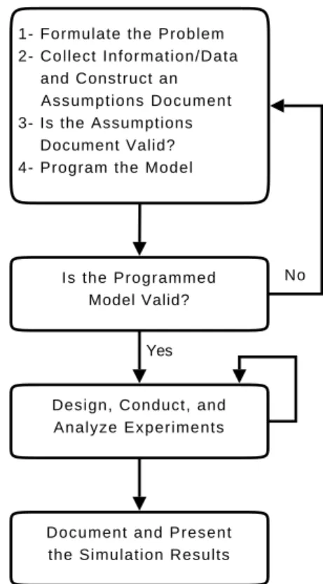
Law presents in [12] a general workflow to build a valid and credible simulation study. Figure 1 resumes Law’s workflow but focus on tasks where instrumentation is needed. The first four tasks of the Law’s workflow lead to a simulation model. Then, the programmed model is checked to state its validity: the simulation model is instrumented and valida-tion results compare results from the real system with results from the simulation model. Next, more simulation experi-ments are designed, conducted and analyzed. The conclu-sions drawn from the simulation results are presented in a document.
In this paper we use the term simulation model to describe the executable program representing the system model un-der study. To design an instrumentation of a system model by following this workflow, most simulators offer a simula-tion API for the declarasimula-tion of observable data within the simulation model. These common practices imply that all the possible observations for a given simulation model need to be decided (and hard coded) at the time the system model is implemented. But, simulation model developers find it difficult to choose which data need to be instrumented, and end-users are reluctant to run simulations collecting data they don’t care about. Moreover, if the resulting simulation
1- Formulate the Problem 2- Collect Information/Data and Construct an Assumptions Document 3- Is the Assumptions Document Valid? 4- Program the Model
Is the Programmed Model Valid?
Design, Conduct, and Analyze Experiments
Document and Present the Simulation Results
No
Yes
Figure 1: Simulation workflow focusing on instru-mentations tasks.
model does not contain the required instrumentation for an analysis, a software evolution is necessary to modify the sim-ulation model. This raises an issue about the credibility of the conclusions drawn from the comparison of simulation results from different simulation models.
Separation of Concerns.
From this perspective, the sepa-ration of concerns between model and instrumentations pro-vides many benefits. For example, keeping the simulation model clear from any instrumentation allows to reuse it in every kind of studies and makes it more understandable. Moreover, instrumenting only the data needed allows to run simulations faster. On large-scale simulations involving many experts, each expert could work on his part. Indeed, it is important for large-scale and distributed simulations to allow instrumentation experts working independently from the simulation modeling expert. This leads to remove de-pendences between tasks of Box 1 and the other boxes in Figure 1.We propose to use the Aspect-Oriented Programming (AOP) paradigm [11] that enables us to separate model-ing concern from instrumentation concern, and to weave the code of the model and the code of the instrumentation on demand. Moreover, we separate the collection of raw instrumentation data (into collectors) from the processing of higher-level instrumentation results (into processors with generic operators). This second separation of concerns is one of the key concepts proposed by the COSMOS framework [5, 16].
From Real to Virtual System.
Before carrying out a sim-ulation study, it is necessary to follow a validation process as mentioned in the second box of Figure 1. The instrumen-tation can help validate a simulation model by comparing simulation results with experiments on a real system. This requires to use firstly the same inputs and secondly the same statistical analysis of the outputs. The best approach would be to use the same validation results process on experimen-tation and simulation. Indeed, a process to validate results that could be applied both on a real system and on a simu-lation model gives more credibility to the simusimu-lation model, and allows extrapolating the findings of a simulation on a real system.The COSMOS framework has been created to process con-text information of real systems during their executions. Using also COSMOS as the instrumentation framework for simulation purposes allows using it both when experiment-ing the real system and simulatexperiment-ing the virtual system.
From Live to Post analysis.
The third box of Figure 1is about the design, the running and the analysis of simu-lation experiments. Running a simusimu-lation may result in a huge amount of simulation data and may then consume a lot of disk space. Moreover, gathering data in a distributed simulation is not trivial and may also consume a lot of net-work bandwidth. After having run experiments, when all the simulation data are collected, a validation phase is nec-essary before they are analyzed. Indeed, a simulation run may produce results that could not be analyzed for instance because the confidence interval is too large or because the duration of the simulation considering the simulation time is too narrow. If so, it is necessary to loop to the third box in order to obtain results that are analyzable. Afterwards, sim-ulation results are analyzed and conclusions can be drawn (fourth box of figure 1).
In order to avoid memory, disk, and bandwidth consump-tion issues, and in order to ease and then optimize the val-idation and analysis processes, we propose to execute these three steps (data gathering, validation of simulation results, and analysis) together during the simulation run (called live analysis). Therefore, data gathering may not store any data on disks but will send them directly to the validation and analysis processors. The validation process dynamically con-trols the analysis process in order to produce results easily understandable. As a consequence, the data flow can be optimized. Moreover, it is easier to replay a study that inte-grates its data processing. Indeed, since statistical analysis are done in live during instrumentation processing, no third-party tool is required. Nevertheless, it is sometimes neces-sary to preserve raw data (e.g. for debugging purposes). Thus, logging capabilities for post analysis is also a require-ment.
COSMOS provides the developer with pre-defined generic operators such as averagers or additioners. Each operator is included into a unit of control called a processor or a node. A node can be finely tuned to be active or passive, block-ing or not in observation or in notification, etc. Therefore, COSMOS allows us to easily build a live analysis on in-strumented data while optimizing data flow. Moreover, we
will show in the next sections how we can easily complement chains of processors that optimize data flows for live analysis with chains of nodes that log raw data for post analysis.
Instrumentation Composition.
Another interestingstrumentation feature is the possibility to write simple in-strumentation processes (including data gathering, valida-tion of simulavalida-tion results, and analysis) and combine them into more complex ones. Benefits are valuable since writing many simple instrumentation processes is easier than writing a complex one. Considering reuse, it is more likely to reuse several times simple and generic instrumentation processes rather than reusing a complex dedicated one. Another case of reuse is the design of a new instrumentation process from an already existing one from a catalogue. Reusing and posing instrumentation process is also an asset when com-paring studies sharing the same instrumentation process. In that case, it is easier to compare and trust the results be-cause validation of simulation results and results analysis are the same among studies.
COSMOS is a component-based framework based on the
Fractal component model [3, 4] and its associated
ar-chitecture description language Fractal ADL [13]. The
Fractalcomponent model is a reflexive component model
providing composition with sharing. Fractal ADL is capa-ble of specifying the reuse of instrumentation processes by the sharing of components since COSMOS concepts (e.g., collectors and processing nodes) are reified as components.
3.
CASE STUDY
As a proof of concept and to show in a practical way how the separation of concerns, the live-post analysis, and the com-position of instrumentations are performed with OSIF, we take the case study of the simulation of a peer-to-peer
sys-tem1. We choose this illustrative example because it shows
the limits of simple instrumentations.
In fact, the goal is to simulate a safe backup storage system on a peer-to-peer network. The model involves N peers and one peer connected through a network. The super-peer has a global vision of the system like in the Edon-key2000 protocol. Each peer could establish communication with any other peers (N ∗ (N − 1) links). The scenario in-volves users, each user is connected to one peer and can push data into the P2P storage system. Data are split into blocks of the same size, each block is fragmented into s frag-ments. From these s fragments, r redundancy fragments are computed. The (s + r) fragments of the data block are dis-tributed on different peers. Any combination of s fragments allows to rebuild the raw data. Therefore, the system tol-erates r failures. Peers are free to leave the system at any time. Peers who disappear are considered dead and reappear empty after a certain period. In that case, a reconstruction mechanism of lost fragments is introduced to ensure data durability.
From this model, several instrumentations can be con-ducted. For instance, to validate results of the simulation model, we want to check that the peer’s lifetime corresponds
to the values that have been specified, to check that the num-ber of fragments corresponds to the numnum-ber of blocks into the system multiplied by (s + r), or to check that the re-constructions only processes critical blocks. When the sim-ulation model is validated, many studies can be conducted, for instance for analyzing the incidence of peers’ lifetime, re-dundancy level, topology of the network of peers, or blocks’ allocation on peers.
For the sake of simplicity, we will focus only on the instru-mentation of the peers’ lifetime that illustrates issues about separation of concerns, optimization of instrumented data flow, and design of complex instrumentation by composi-tion. To prototype our solution, we have used the OSA simulator.
4.
OPEN SIMULATION
INSTRUMENTA-TION FRAMEWORK
Open Simulation Instrumentation Framework (OSIF) is a framework to design, conduct, validate and analyze results of experiments. OSIF is based on several strong software engineering concepts and open frameworks such as AOP,
Fractal ADLand COSMOS. OSIF is architectured around
four principles:1)separation of concerns between simulation
concern and instrumentation concern,2) live-post
process-ing of instrumented data, 3) reuse of existing
instrumen-tation between real or simulated systems, and4) easy
de-sign of complex instrumentation processings by composition. The first principle fosters the separation of instrumentation concern from modeling concern, enabling the reuse of in-strumentation code and facilitating software evolution. The second principle enables the optimization of the transmis-sion, the storage, and the processing of instrumented data. The third principle also leverages the confidence in simula-tion analysis results and conclusion thanks to the fact that instrumentations have been used and validated repeatedly both on real and simulated systems. The fourth principle allows a better understanding of the instrumentation pro-cess, and to conduct better and much more complex instru-mentation with fewer software defaults.
In this section, we begin with a short introduction to the principles of the COSMOS framework. Next, we explain how to handle issues presented in Section 2 with OSIF.
4.1
COSMOS
COSMOS (COntext entitieS coMpositiOn and Sharing) [5, 16, 15] is a LGPL component-based framework for managing context data in ubiquitous applications. Context manage-ment is (i) user and application centered to provide informa-tion that can be easily processed, (ii) built from composed instead of programmed entities, and (iii) efficient by mini-mizing the execution overhead. The originality of COSMOS is to use a component-based approach for encapsulating fine-grain context data, and to use an architecture description language (ADL) for composing these context data compo-nents. By this way, we foster the design, the composition, the adaptation and the reuse of context management poli-cies. In the context of OSIF, context data components be-come instrumentation data components.
The COSMOS framework is architectured around the
fol-lowing three principles that are brought into play in OSIF: the separation of data gathering from data processing, the systematic use of software components, and the use of soft-ware patterns for composing these components. The first principle supports the clean separation between data gath-ering that may depend upon the simulation framework and data processing that is simulation framework
agnos-tic. The second principle, software components, fosters
reuse everywhere. Finally, the third principle promotes the architecture-based approach “composing rather than pro-gramming”. The COSMOS framework is implemented on top of the Fractal component ecosystem with the message oriented middleware (MOM) DREAM [14].
4.2
Separation of Concerns
In OSIF, the separation between simulation and instrumen-tation concerns is performed using the Aspect-Oriented Pro-gramming (AOP) paradigm and the COSMOS’ concept of the “collector”.
Aspect-Oriented Programming.
AOP [11] is a softwareengineering technique for modularizing applications
bring-ing many concerns into play. The general idea is that,
whatever the domain, large applications have to address dif-ferent concerns such as data management, security, GUI, data integrity. Using only procedural or object orientations, these different concerns cannot always be cleanly separated from each other and, when applications evolve and become more complex, concerns end up being intertwined, called the “spaghetti” code problem. AOP promotes three principles. Firstly, functional or extra-functional aspects of an applica-tion should be designed independently from an applicaapplica-tion core and so the application design is easier to understand. Secondly, it is not easy to modularize common-interest con-cerns used by several modules, like logging service. Those cutting concerns can be described using AOP cross-cutting expressions that encapsulate each concern in one place. Thirdly, AOP favors inversion of control principle. Inversion of Control (IoC) is a design pattern attempting to remove all dependencies from the business code by putting them in a special place where the goal is only to manage dependencies. Considering a simple example of a lamp con-trolled by a switch, in basic object-oriented programming, the control of the lamp is placed in the code of the switch. Using the inversion of control principle with AOP the con-trol of the lamp is no longer in the code of the switch but in a dedicated aspect that will make the connection between the switch and lamp. This results in a better separation of concerns and reusability.
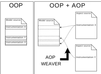
Instrumentation is a cross-cutting concern because many parts of the simulation model need to be introspected and complemented with instrumentation concern. The left part of Figure 2 illustrates how the instrumentation concern pollutes the modeling code when using traditional Object-Oriented Programming (OOP). The code is hard to read and it is hard to figure out where the code of the model is. The right part of Figure 2 illustrates how to avoid this drawback by reorganizing the instrumentation concern into separate source code files (aspects). The arrow represents the action of the AOP weaver which is a tool that is re-sponsible for binding the aspects with the modeling code on
I n s t r u m e n t a t i o n X
I n s t r u m e n t a t i o n X Instrumentation Y
Model source Model source
I n s t r u m e n t a t i o n X Instrumentation Y
OOP + AOP
OOP
Aspect source Aspect sourceAOP
WEAVER
Figure 2: Separation of concerns using AOP.
demand (and possibly dynamically). This keeps the code of the model concise and stripped from the instrumentation code.
As an example, Listing 1 illustrates a Java class Peer with two methods: boot() and halt(). Each method has some modeling code and call the instrumentation framework (crosscuting concern). The instrumentation code pollutes the modeling code as illustrated on the left part of Figure 2. Indeed, Java class Peer invoke method write(message) which is part of the instrumentation framework represented here by the Sampler object. Sampler is connected to the simula-tor engine and writes on disk the simulation time and the message.
Listing 1: Peer Java class without separation of con-cerns. p u b l i c c l a s s P e e r{ S a m p l e r s a m p l e r; S t r i n g p e e r n a m e; p u b l i c void b o o t( ) { [ . . . ] // modeling code s n i p p e d s a m p l e r. w r i t e ( p e e r n a m e+” b o o t ” ) ; } p u b l i c void h a l t( ) { [ . . . ] // modeling code s n i p p e d s a m p l e r. w r i t e ( p e e r n a m e+” h a l t ” ) ; } }
Thanks to AOP, it is possible to separate modeling concern from instrumentation concern. The aspect of Listing 2 writ-ten in AspectJ shows how to isolate the instrumentation concern in a separate module as illustrated on the right part of Figure 2. The aspect peer instrumentation calls the instru-mentation framework right after the execution of methods boot() and halt().
Therefore, Listing 3 illustrates the same modeling code stripped from instrumentation concern.
Listing 2: AspectJ aspect to observe Peer class. p u b l i c aspect p e e r _ i n s t r u m e n t a t i o n { S a m p l e r P e e r. s a m p l e r ; a f t e r( P e e r p e e r ) : execution ( void P e e r . b o o t ( ) ) && t h i s ( p e e r ) { s a m p l e r. w r i t e ( p e e r n a m e+” b o o t ” ) ; } a f t e r( P e e r p e e r ) : execution ( void P e e r . h a l t ( ) ) && t h i s ( p e e r ) { s a m p l e r. w r i t e ( p e e r n a m e+” h a l t ” ) ; } }
Listing 3: Java class with separation of concerns. p u b l i c c l a s s P e e r{ S t r i n g n a m e; p u b l i c void b o o t( ) { [ . . . ] // modeling code s n i p p e d } p u b l i c void h a l t( ) { [ . . . ] // modeling code s n i p p e d } }
Since only the required instrumentation aspect is weaved to the simulation model, the execution of the simulation runs faster. Moreover, software evolutions of the simula-tion model and the instrumentasimula-tion are facilitated. Finally, instrumentation processing can be developed independently by instrumentation experts and reused more easily.
COSMOS Collector.
The lower layer of the COSMOSframework defines the notion of a data collector. In the con-text of ubiquitous applications, data collectors are software entities that provide raw data from the environment. In M&S, the environment is the simulated model under study. A data collector retrieves instrumented data from a simula-tion and provides them to the data processors. COSMOS collectors are generic and the data structure to be pushed by the advice code of the instrumentation aspect is an ar-ray of Object. Therefore, COSMOS collectors and AOP instrumentation advice s perform the junction between the simulation framework and instrumented data processors of OSIF.
4.3
From Live to Post Analysis
We propose to reuse some concepts of COSMOS, like con-cepts of data processor and data policy to analyze simulation data in live but also to log the raw simulation data while preserving optimization on data flow.
COSMOS processor.
We have seen that the lower layer ofthe COSMOS framework defines the notion of data collec-tor. The middle layer of the COSMOS framework defines the notion of a data processor, named context processor in COSMOS. Data processors filter and aggregate raw data coming from data collectors. The role of a data processor is
to compute some high-level numerical or discrete data from raw numerical data outputted either by data collectors or other data processors. Therefore, data processors are or-ganized into hierarchies with the possibility of sharing. A data processor or node of this graph can be parameterized to be passive or active, blocking or not in observation or in notification.
• Passive Vs. active. A passive node obtains
sim-ulation data upon demand; a passive node must be invoked explicitly by another node. An active node is associated to a thread and initiate the gathering and/or the treatment of simulation data. The thread may be dedicated to the node or be retrieved from a pool. A typical example of an active node is the cen-tralization of several types of simulation data, the pe-riodic computation of a higher-level simulation data, and the provision of the latter information to upper nodes, then isolating a part of a hierarchy from too frequent and numerous calls.
• Observation Vs. notification. The simulation re-ports containing simulation data are encapsulated into messages that circulate from the leave nodes to the root nodes of the hierarchies. When the circulation is initiated at the request of parent nodes or client appli-cations, it is an observation. In the other case, this is a notification.
• Blocking or not. During an observation or a notifi-cation, a node that treats the request can be blocking or not. During an observation, a non-blocking node begins by requesting a new observation report from each of its child nodes, and then updates its simula-tion data before answering the request of the parent node or the client application. During a notification, a non-blocking node computes a new observation re-port with the new simulation data just being notified, and then notifies the parent node or the client applica-tion. In the case of a blocking node, an observed node provides the most up-to-date simulation data that it possesses without requesting child nodes, and a noti-fied node updates its state without notifying parent nodes.
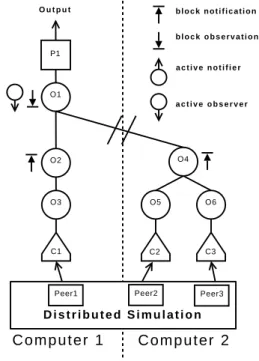
Figure 3 illustrates how to use COSMOS data processors to instrument and compute outputs in a distributed sim-ulation. A distributed simulation involving three peers is executed on two computers. This instrumentation produces as output the min, max, and average lifetime of peers. Each peer is connected to a data collector. Data collectors receive simulation data every time the state of the attached peer changes. Then, collectors push the simulation data to the data processors in which there are enclosed. Data processors O3, O5, and O6 compute the lifetime of peers, that is the dif-ference between the starting up and the shutting down, and send these simulation data to processors O2 and O4. Those processors gather these simulation data from all the peers of the same host and compute the min, max, sum of the lifetimes of peers and the total number of times lifetime has been calculated. Since the latter processors are blocking in notification, the flow of data is stopped. In conclusion, data
processors O2 or O4 are updated every time a peer lifetime is computed and gather simulation data collected on every peer executing in a host.
Data processor O1 is responsible for gathering simulation data at the global level, that is for all the peers of all the hosts. This node is active in observation but blocking, thus meaning that it periodically requests simulation data from data processors 02 and 04.
C2 C3 C1 P1 O3 O5 O6 O2 O4 O1 b l o c k n o t i f i c a t i o n b l o c k o b s e r v a t i o n a c t i v e n o t i f i e r a c t i v e o b s e r v e r
C o m p u t e r 1
C o m p u t e r 2
D i s t r i b u t e d S i m u l a t i o n O u t p u tPeer1 Peer2 Peer3
Figure 3: Graphical representations of data process-ing in a distributed simulation.
Therefore, considering this live analysis, the disk overhead to store simulation data can be minimum if we store only the final result provided by node O1. Concerning the band-width overhead, it depends upon the number of requests performed by node O1 and upon the amount of simulation data transferred from node O4 to O1. Considering the
previ-ous simulation involving N peers (N′is the number of peers
on Computer2), each peer being started up and shut down T times during the simulation. A basic instrumentation would have written N ∗ T times the peer name, the action (boot or halt) and the simulation time on disk. The same
instrumen-tation would have transferred N′
∗ T times the peer name, the action (boot or halt) and the simulation time thru the network. For large-scale simulations, the amounts of data will be huge. Using OSIF, we can easily build a live anal-ysis instrumentation that directly write only the min, max, and average lifetime of peers on disk, and transfers the min, max, sum of the lifetimes of peers and the total number of times lifetime has been calculated. thru the network. More-over, live analysis have its own thread, so we do not notice any CPU overhead on a Core2Duo computer. For exam-ple, running a local simulation involving 1000 peers during 5 years takes 23 seconds to instantiate and 70 seconds to execute with live analysis of peers lifetime. With basic log-ging of the raw simulation data the same simulation takes
14 seconds to instantiate and 70 seconds to execute. The difference represents the overload due to the instantiation of COSMOS nodes and collectors.
COSMOS instrumentation policy.
The upper layer of theCOSMOS framework defines the notion of a context policy that translated into the concept of instrumentation in OSIF. COSMOS instrumentation policy abstracts simulation data provided to the user/application, that is instrumentation policies are the “entry points” to the graph of processing nodes. We use instrumentation policies to translate instru-mentation data provided by COSMOS processors into an understandable format: textual, graphical, or third-party tools compliant.
Let’s take the example of Figure 3. The goal now is to log simulation data in order to have the complete peers’ connec-tion and disconnecconnec-tion history. The node O1 aggregates and merges simulation data from nodes O2 and O4 and pushes them to the instrumentation policy P1. The instrumentation policy may then decides the output format, for instance for being able to process them using OMNeT++ analysis tool Scave [17]. Scave helps the user to process and visualize simulation results saved into vector and scalar files. So, the instrumentation policy P1 translates simulation data out-putted by node O1 into vector or scalar files understandable by Scave. Thus, we can latter post-analyze our data using Scave.
We have seen how using COSMOS data processors and poli-cies we can design a live analysis or a logging system. Log-ging raw data is necessary in certain cases such as debugLog-ging but live analysis allows for disk usage and network band-width usage optimizations. The CPU overhead may be sig-nificant on large instrumentations with lots of computations: in the worst case, it will be the same as the computation needed by a post analyze. Thus, OSIF allows designing in-strumentations taking into account the topology of the simu-lation and optimizing the data flow, but also it can produce results consistent with existing tools in order to compare simulation studies results.
4.4
Composition of instrumentations
In this section, we show how to use the architecture de-scription language of Fractal (Fractal ADL) for sharing, reuse and mix COSMOS-based instrumentation processing: collectors, data processors, and instrumentation policies.
Component-based Architecture.
Being based onCOS-MOS, OSIF benefits from the three principles of separation of concerns, isolation and composability of the component-based software engineering approach: in COSMOS, every data collector and every data processor is a software compo-nent. By connecting these components, we define assemblies that gather all the information needed to implement a spe-cific instrumentation policy. COSMOS is implemented with the Fractal component model and instrumentation policies are specified using Fractal ADL. Designers of intrumen-tation policies are able to describe complex hierarchies of data processors by taking advantage of the two main char-acteristics of Fractal: hierarchical component model with
sharing.
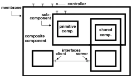
Figure 4: Graphical notations of the Fractal compo-nent model.
As depicted in Figure 4, a component is a software entity that provides and requires services. The contracts of these services are specified by interfaces. Fractal distinguishes server interfaces that provide services and client interfaces that specify the required services. A component encapsu-lates a content. It is then possible to define hierarchies of components offering views at different level of granularity. Hierarchies are not solely trees since sub-components shared by several composites. The notion of sharing of components naturally expresses the sharing of system resources (mem-ory, threads, etc.). Components are assembled with bind-ings, which represent a communication path from a client interface to a (conformant) server interface. Moreover, com-positions of components are described with an Architecture Description Language (ADL). Without lack of generality, in the sequel, we use the graphical notations of the Fractal component model, as illustrated in Figure 4, and the lan-guage Fractal ADL [13] that is based on XML.
Architecture Description Language.
Fractal ADLis aXML language to describe the architecture of a Fractal ap-plication: components’ topology (or hierarchy), relationship between client interfaces and server interfaces, name and initial value of components’ attributes. A Fractal ADL definition can be divided into several sub-definitions placed into several files. Thus, Fractal ADL allows the separa-tion of concerns because applicasepara-tion definisepara-tion can be split into multiple files. Moreover, Fractal ADL supports a mechanism to ease the extension and redefinition through inheritance. Extension and redefinition allow the reuse (of a part or the whole) of existing instrumentation policies writ-ten using Fractal ADL. When a definition B exwrit-tends a definition A, B possesses all the elements defined in defini-tion A, like an internal copying mechanism. Moreover, if definition B defines an element that has the same name in definition A, B’s definition overrides A’s one. The extension mechanism enables us to create a new definition by compo-sition of existing definitions. Listing 4 illustrates a Fractal
ADL definition of the live analysis of a peer. This
defini-tion takes one argument and is composed of four Fractal components: a collector and a data processor parameterized with the name of the peer used in argument and allowing to compute the lifetime of a peer, a data processor com-puting the average lifetime, and an instrumentation policy presenting the result.
Listing 4: Fractal ADL definition of a live analysis of a peer lifetime. <d e f i n i t i o n name=” P e e r L i f e t i m e ” arguments=” peername ”> <component name=” O u t p u t P o l i c y ” [ . . . ] <!−− A D L c o d e s n i p p e d −−> <component name=” A v e r a g e L i f e t i m e ” [ . . . ] <!−− A D L c o d e s n i p p e d −−>
<component name=” L i f e t i m e O f $ { peername } ” [ . . . ] <!−− A D L c o d e s n i p p e d −−>
<component name=” C o l l e c t o r O f $ { peername } ” [ . . . ] <!−− A D L c o d e s n i p p e d −−> </component> </component> </component> </component> </d e f i n i t i o n >
Figure 5 illustrates the multiple extension capability of
Fractal ADL. At the top, we have a Fractal ADL
def-inition extending the Fractal ADL defdef-inition of Listing 4 with two different parameters. At the bottom, we have the resulting instrumentation policy. We can see that the data processors LifetimeOfPeer1 and LifetimeOfPeer2 are both en-capsulating the data processor AverageLifetime. This can be done thanks to the inheritance mechanism of Fractal
ADL. From this example, it’s easy to imagine and design
more complex composition such as composition of several live analysis (lifetime, bandwidth, . . . ) and logging to post analyze simulation data.
The extension capabilities of Fractal ADL allow, as il-lustrated in the example defined in figure 5, to merge com-ponents. The merging process allows to update and extend already defined component. Therefore, it is possible to reuse and extend existing instrumentation and configure it. This can range from a simple update of parameters until the re-placement or addition of management contexts.
<d e f i n i t i o n name=”C o m p o s i t i o n ” e x t e n d s=P e e r L i f e t i m e ( p e e r 1 ) , P e e r L i f e t i m e( p e e r 2 )> </d e f i n i t i o n > CollectorOfpeer1 CollectorOfpeer2 LifetimeOfpeer1 LifetimeOfpeer2 AverageLifetime OutputPolicy
Figure 5: Fractal ADL composition mechanism and the resulting COSMOS design.
There are several benefits to using the extension and the redefinition mechanisms of Fractal ADL. Firstly, writing many simple instrumentations is easier for maintenance than
writing a complex instrumentation from scratch. Secondly, there is more chance to reuse generic simple instrumenta-tions rather than a complex dedicated one. Thirdly, it is easier to compare and have confidence in results when in-strumentation and statistical analysis are the same among studies. In order to do this, since a simulation model is the composition of existing models and new models, the cor-responding instrumentation may also be the composition of existing instrumentations and new instrumentations. There-fore, each simulation model should be accompanied by one or more instrumentations that could be reused —i.e., at least the instrumentation used to validate the simulation model.
4.5
From Real to Virtual System
In OSIF, we use COSMOS to process simulation data. As mentioned in Section 2, it would be appropriate to com-pare simulation results with the results of an experiment. COSMOS has originally been developed to manage context
data in ubiquitous applications [3, 4, 15]2. So, OSIF can
naturally be used for instrumenting both real applications and simulations of real applications. As a consequence, the validation of simulation models is much more effective, less buggy. Therefore, the level confidence in the validation pro-cess increases.
5.
RELATED WORKS
Although designing, conducting and analyzing an experi-ment are not trivial tasks, there are few literatures
address-ing those issues. In practice, most users simply update
the model or simulator to consider their instrumentations. Those practices, however, questions the credibility of results. In [18], Zeigler and al. are the first to take into account those questions. They propose the concept of the experimental frame into the DEVS formalism. A frame generates input to the model, monitors an experiment to see the desired experimental conditions are met and observes and analyzes the model output. Thus, the experimental frame not only instrument but also drive the simulation. Nevertheless, the experimental frame does not consider how model outputs are computed. In fact, to manage output using the experimental frame, the model needs to produce simulation output on the output port. Therefore, the model needs to forward on its output port internal data to observe. Thus, the model mix modeling concern with instrumentation concern.
In [1], Andrad´ottir addresses the management of simulation
data flow. He describes techniques to reduce the computa-tional complexity of dynamic observation and on-line statis-tics computation. In [10], Himmelspach and al. propose in JamesII a simple architecture to handle the transmission during the simulation of the data across the network, to their storage destination. In both cases, they do not con-sider to separate the data gathering concern from the mod-eling concern but propose an interesting solution to manage simulation data.
In [9], Gulyas and Kozsik address the problematic of separa-tion of concerns in simulasepara-tion using AOP. They do not focus
2See also the following projects: Cappucino on mobile
com-merce (http://www.cappucino.fr/), and Totem on perva-sive gaming
generally on instrumentation and analysis problematic but on the use of AOP to gather data.
In [17], Varga and Hornig address the problematic of results’ analysis. They propose Scave, a tool to post analyzes simu-lation data. Scave can apply a batch of analysis to several simulation data files. This favors the comparison between similar studies by using the same analysis process on several simulation outputs but does not raise questions about data gathering.
We propose to reuse all of these principles in a single frame-work. In fact, we propose to separate the modeling con-cern and the instrumentation concon-cern using AOP, reduce the computational complexity of dynamic observation and on-line statistics computation and transmit the data across the network to their storage destination using COSMOS. Moreover, it is possible to save the simulation data in any format. Therefore, using the standard format from Om-net++, we are able to use Scave to post process simulation data.
6.
CONCLUSIONS AND PERSPECTIVES
As a conclusion, we have shown in this paper OSIF, a frame-work to design, conduct and analyze experiments thanks to several software engineering principles and framework such as AOP, COSMOS and Fractal ADL. OSIF is a generic solution that could be integrated in every simulator. OSIF has been used successfully through the large-scale simula-tion presented in Secsimula-tion 3. Benefits of OSIF are multiple: (i) OSIF allows a complete separation of concerns between modeling and instrumentation; (ii) OSIF favors validation results by allowing the sharing of analysis between the real system and the simulated system; (iii) OSIF allows to man-age and optimize the flow of simulation data whatever we want to live analyze or post analyze simulation data; and (iv) OSIF allows to design and compose complex instrumen-tations in a simple way.
The use of the OSIF framework is based on the use of AOP and COSMOS. Since AOP is available for most program-ming languages, OSIF could be used whatever the simulator and the language used. COSMOS collectors are written in Java, but there already exist several ways to integrate non-Java languages, for example, using JNI. The next step to the success is to unite a community around OSIF to build and share COSMOS components in order to enrich the ex-perience of the end-user.
To enrich the OSIF experience, we are planning future works. The first one is derived from the fact that exten-sion and redefinition mechanisms of Fractal ADL can lead to unintended results because of side effects being difficult to predict. A tool for describing, analyzing and verifying instrumentation as one currently developed by COSMOS (COSMOS DSL) will retain the advantages while avoiding disadvantages. Then, a medium term project is to build on top of the COSMOS instrumentation policy a tool to drive simulation experiments. We plan to bring into play the principles that Himmelspach explained in [10]. Indeed, COSMOS offers all we need to drive simulation such as con-trolling the number of runs necessary to obtain the expected confidence intervals or automatically cut the beginning of a
simulation or refining inputs to obtain the best inputs com-bination for a study.
7.
ACKNOWLEDGMENTS
This work was partially funded by the European project IST/FET AEOLUS, the ANR project SPREADS and the ARC INRIA project BROCCOLI.
8.
REFERENCES
[1] S. Andrad´ottir. Handbook of Simulation, chapter
9-Simulation Optimization, pages 307–334. EMP & Wiley, 1998.
[2] J. Banks, J. S. Carson II, B. L. Nelson, and D. M. Nicol. Discrete-Event System Simulation. Prentice Hall, 5th edition, 2009.
[3] E. Bruneton, T. Coupaye, M. Leclercq, V. Qu´ema, and J.-B. Stefani. An Open Component Model and its Support in Java. In Proc. 7th International
Symposium on Component-Based Software Engineering, volume 3054 of Lecture Notes in Computer Science, pages 7–22, May 2004.
[4] E. Bruneton, T. Coupaye, M. Leclercq, V. Qu´ema, and J.-B. Stefani. The Fractal Component Model and Its Support in Java. Software—Practice and Experience, special issue on Experiences with Auto-adaptive and Reconfigurable Systems, 36(11):1257–1284, Sept. 2006. [5] D. Conan, R. Rouvoy, and L. Seinturier. Scalable
Processing of Context Information with COSMOS. In J. Indulska and K. Raymonds, editors, Proc. 6th IFIP WG 6.1 International Conference on Distributed Applications and Interoperable Systems, volume 4531 of Lecture Notes in Computer Science, pages 210–224, Paphos, Cyprus, June 2007. Springer-Verlag.
[6] O. Dalle. OSA: an Open Component-based Architecture for Discrete-Event Simulation. In 20th European Conference on Modeling and Simulation (ECMS), pages 253–259, Bonn, Germany, May 2006. [7] O. Dalle and C. Mrabet. An instrumentation
framework for component-based simulations based on the separation of concerns paradigm. In Proc. of 6th EUROSIM Congress (EUROSIM2007), Ljubljana, Slovenia, September 9-13 2007.
[8] R. M. Fujimoto. Parallel and distributed simulation systems. Wiley Series on Parallel and Distributed Computing. J Wiley & Sons, 2000.
[9] L. Gulyas and T. Kozsik. The Use of Aspect-Oriented Programming in Scientific Simulations. In Proceedings of Sixth Fenno-Ugric Symposium on Software
Technology, Estonia. Citeseer, 1999.
[10] J. Himmelspach, R. Ewald, and A. M. Uhrmacher. A flexible and scalable experimentation layer. In S. Mason, R. Hill, L. M¨onch, O. Rose, T. Jefferson, and J. Fowler, editors, Proc, of the 2008 Winter Simulation Conference (WSC’08), pages 827–835, Miami, FL, Dec. 2008.
[11] G. Kiczales, J. Lamping, A. Mendhekar, C. Maeda, C. V. Lopes, J.-M. Loingtier, and J. Irwin.
Aspect-oriented programming. In European Conference on Object-Oriented Programming, ECOOP’97, volume 1241 of LNCS, pages 220–242, Jyv¨askyl¨a, Finland, June 1997. Springer-Verlag.
[12] A. Law. Simulation Modeling and Analysis. McGraw-Hill, 2006.
[13] M. Leclercq, A. ¨Ozcan, V. Qu´ema, and J.-B. Stefani.
Supporting Heterogeneous Architecture Descriptions in an Extensible Toolset. In Proc. 29th ACM International Conference on Software Engineering, (USA), May 2007.
[14] M. Leclercq, V. Qu´ema, and J.-B. Stefani. DREAM: a Component Framework for the Construction of Resource-Aware, Configurable MOMs. IEEE Distributed Systems Online, 6(9), Sept. 2005. [15] D. Romero, R. Rouvoy, S. Chabridon, D. Conan,
N. Pessemier, and N. Seinturier. Enabling
Context-Aware Web Services: A Middleware Approach for Ubiquitous Environments. Chapman and
Hall/CRC, 2009.
[16] R. Rouvoy, D. Conan, and L. Seinturier. Software Architecture Patterns for a Context Processing Middleware Framework. IEEE Distributed Systems Online, 9(6), June 2008.
[17] A. Varga and R. Hornig. An overview of the
OMNeT++ simulation environment. In Proceedings of the 1st international conference on Simulation tools and techniques for communications, networks and systems & workshops, page 60. ICST (Institute for Computer Sciences, Social-Informatics and Telecommunications Engineering), 2008.
[18] B. P. Zeigler. Theory of Modelling and Simulation. Krieger Publishing Co., Inc., Melbourne, FL, USA, 1984.