HAL Id: hal-01099544
https://hal.archives-ouvertes.fr/hal-01099544
Submitted on 7 Jan 2015
HAL is a multi-disciplinary open access
archive for the deposit and dissemination of sci-entific research documents, whether they are pub-lished or not. The documents may come from teaching and research institutions in France or abroad, or from public or private research centers.
L’archive ouverte pluridisciplinaire HAL, est destinée au dépôt et à la diffusion de documents scientifiques de niveau recherche, publiés ou non, émanant des établissements d’enseignement et de recherche français ou étrangers, des laboratoires publics ou privés.
Sea-salt injections into the low-latitude marine
boundary layer: The transient response in three Earth
system models
K. Alterskjær, J.E. Kristjánsson, Olivier Boucher, H. Muri, U. Niemeier, H.
Schmidt, M Schulz, C. Timmreck
To cite this version:
K. Alterskjær, J.E. Kristjánsson, Olivier Boucher, H. Muri, U. Niemeier, et al.. Sea-salt injections into the low-latitude marine boundary layer: The transient response in three Earth system models. Journal of Geophysical Research: Atmospheres, American Geophysical Union, 2013, 118 (21), pp.12195-12206. �10.1002/2013JD020432�. �hal-01099544�
Sea-salt injections into the low-latitude marine boundary layer:
The transient response in three Earth system models
Kari Alterskjær,1Jón Egill Kristjánsson,1Olivier Boucher,2Helene Muri,1 Ulrike Niemeier,3Hauke Schmidt,3Michael Schulz,4and Claudia Timmreck3
Received 27 June 2013; revised 30 September 2013; accepted 21 October 2013.
[1] Among proposed mechanisms for counteracting global warming through solar radiation
management is the deliberate injection of sea salt acting via marine cloud brightening and the direct effect of sea-salt aerosols. In this study, we show results from multidecadal simulations of such sea-salt climate engineering (SSCE) on top of the RCP4.5 emission scenario using three Earth system models. As in the proposed“G3” experiment of the Geoengineering Model Intercomparison Project, SSCE is designed to keep the top-of-atmosphere radiative forcing at the 2020 level for 50 years. SSCE is then turned off and the models run for another 20 years, enabling an investigation of the abrupt warming associated with a termination of climate engineering (“termination effect”). As in former idealized studies, the climate engineering in all three models leads to a significant suppression of evaporation from low-latitude oceans and reduced precipitation over low-latitude oceans as well as in the storm-track regions. Unlike those studies, however, wefind in all models enhanced evaporation, cloud formation, and precipitation over low-latitude land regions. This is a response to the localized cooling over the low-latitude oceans imposed by the SSCE design. As a result, the models obtain reduced aridity in many low-latitude land regions as well as in southern Europe. Terminating the SSCE leads to a rapid near-surface temperature increase, which, in the Arctic, exceeds 2 K in all three models within 20 years after SSCE has ceased. In the same period September Arctic sea ice cover shrinks by over 25%.
Citation: Alterskjær, K., J. E. Kristja´nsson, O. Boucher, H. Muri, U. Niemeier, H. Schmidt, M. Schulz, and C. Timmreck (2013), Sea-salt injections into the low-latitude marine boundary layer: The transient response in three Earth system models, J. Geophys. Res. Atmos., 118, doi:10.1002/2013JD020432.
1. Introduction
[2] The concept of “climate engineering” (CE) or
geo-engineering refers to a deliberate manipulation of the climate in order to avoid the most severe consequences of global warming [Crutzen, 2006]. It has gained increased scientific interest over the past decade, as global emissions of long-lived greenhouse gases, in particular CO2, continue to soar, raising
concerns that the“2°C target” may become unachievable by mitigation alone [Rogelj et al., 2010]. Recent extreme summer heat waves over the midlatitude continents have been statisti-cally linked to global warming [Coumou and Rahmstorf,
2012], further raising awareness of some of the manifestations of global warming.
[3] Solar radiation management (SRM) is a subset of CE
techniques that involves increasing the reflection of solar radi-ation from the Earth system in order to limit global warming. Among proposed SRM techniques is marine cloud brighten-ing (MCB),first proposed by Latham [1990]. MCB seeks to exploit the first aerosol indirect effect [Twomey, 1977] by which an increase in the concentration of cloud condensation nuclei (CCN) may increase the number of droplets in a cloud, thereby increasing their total surface area and hence the cloud albedo. Droplets of sea water would be sprayed into the air, e. g., by unmanned vessels [Salter et al., 2008], and as the sea water evaporates it leaves behind sea-salt particles which may be lifted into above lying cloud decks and increase their albedo. This process may also lead to a second indirect effect in which the decreased size of the cloud droplets leads to suppressed precipitation release and therefore to an increase in cloud lifetime and optical depth [Albrecht, 1989].
[4] Several model studies have looked at the radiative and
the climatic impact of such climate manipulation. Latham et al. [2008]; Jones et al. [2009] and Rasch et al. [2009] modeled MCB using simplified assumptions when prescribing certain cloud droplet numbers resulting from the sea-salt seeding, while Korhonen et al. [2010]; Partanen et al. [2012]; Jones and Haywood [2012]; Alterskjær et al. [2012] 1Department of Geosciences, University of Oslo, Oslo, Norway.
2
Laboratoire de Météorologie Dynamique, IPSL/CNRS, Université Pierre et Marie Curie, Paris, France.
3
Max Planck Institute for Meteorology, Hamburg, Germany.
4Norwegian Meteorological Institute, Oslo, Norway.
Corresponding author: J. E. Kristjánsson, Department of Geosciences, University of Oslo, Oslo, Norway. ( jegill@geo.uio.no)
©2013 The Authors. Journal of Geophysical Research: Atmospheres published by Wiley on behalf of the American Geophysical Union. This is an open access article under the terms of the Creative Commons Attribution-NonCommercial-NoDerivs License, which permits use and dis-tribution in any medium, provided the original work is properly cited, the use is non-commercial and no modifications or adaptations are made. 2169-897X/13/10.1002/2013JD020432
and Alterskjær and Kristjánsson [2013] performed model studies in which sea-salt particles were emitted from the sea surface in an attempt to simulate more realistically the physical processes involved. They all found significant cooling effects on the climate, due to the aerosol indirect effect increasing cloud albedo, but large spatial variations were found in the temperature signals. Rasch et al. [2009] found that MCB could restore the globally averaged near-surface temperature and pre-cipitation to present-day values but not simultaneously. Partanen et al. [2012] and Jones and Haywood [2012] also studied the radiative impact of clear-sky reflection of solar radiation by the sea-salt aerosols themselves, referred to as the direct effect of the sea salt. They found that this effect contributed significantly to the total radiative impact of sea-salt seeding. Online interactive simulations [Bala et al., 2011; Hill and Ming, 2012; Baughman et al., 2012] make it possible to study the climate response to this kind of manipulation, includ-ing possible side effects and feedbacks. A problem is that some of these responses and feedbacks may be model dependent. Another challenge is that so far no common experimental de-sign has been used, and therefore comparison of the different studies is difficult. To alleviate these problems, a multimodel approach with a common experimental setup was needed.
[5] We herein present results from what to our knowledge is
thefirst coordinated multimodel study of sea-salt climate engi-neering (SSCE). Three Earth system models (ESMs) are used to simulate a canceling of the forcing from the RCP4.5 sce-nario by sea-salt seeding. The objective of the multimodel ap-proach is to study what simulated CE climate responses are robust between the models. In particular, we investigate radia-tive effects and impacts on the hydrological cycle, near-surface air temperatures, and surfacefluxes. GeoMIP (Geoengineering Model Intercomparison Project) [Kravitz et al., 2011] is cur-rently following up our study and previous simpler GeoMIP G1 and G2 intercomparisons, in which CO2forcing was
can-celed by reductions in the solar constant, by creating a set of well-defined SSCE experiments to be performed by participat-ing modelparticipat-ing groups in GeoMIP [Kravitz et al., 2013].
[6] The participating models and the experimental setup
are described more closely in section 2, while results are presented and discussed in section 3. We summarize and conclude in section 4.
2. Models and Experimental Setup
[7] Three state-of-the-art Earth system models were used in
this study; the Institut Pierre Simon Laplace ESM
(IPSL-CM5A [Dufresne et al., 2013]), the Max Planck Institute ESM (MPI-ESM [Giorgetta et al., 2013]), and the Norwegian ESM (NorESM [Bentsen et al., 2013]). The main characteris-tics of the models are listed in Schmidt et al. [2012, Table 1], which shows that the models do not share any main compo-nents and they are run at slightly different resolutions. For the atmosphere, the IPSL-CM5A runs at 2.5° × 3.75° with 39 ver-tical layers up to 65 km, the MPI-ESM runs at a T63 spectral truncation with 47 layers in the vertical ending at 0.01 hPa, and the NorESM runs at 1.9° × 2.5° with 26 vertical layers up to ~2 hPa. The ocean component has 96 × 95 grid points and 39 layers in the IPSL-CM5A, ~1.5° × 1.5° and 40 layers in the MPI-ESM, and ~1° × 1° and 70 layers in the NorESM. The advantage of having such diversity in model components and resolutions is that this will increase confidence in results supported by all three models [Schmidt et al., 2012]. This study does not include an evaluation of the models themselves as this is already done elsewhere.
[8] The SSCE experiment is designed so as to cancel the
globally averaged radiative forcing relative to 2020 associated with the RCP4.5 scenario [Moss et al., 2010]. This resembles what is proposed for the GeoMIP G3 experiment [Kravitz et al., 2011], in which injected stratospheric sulfur is to cancel the RCP4.5 forcing, and we therefore denote our experiment G3-SSCE. The SSCE experiment was initialized in 2020 from a reference simulation of RCP4.5, and the tabulated forcing of the RCP4.5 was balanced by SSCE until 2070, when the SSCE was turned off. The simulations continued for another 20 years to enable investigation of the termination effect from this type of CE. We note that the RCP4.5 radiative forcing change from 2020 to 2070 is +1.64 W m 2, so that a much
weaker CE is needed in the G3 experiments than in the simpler G1 experiment, where the forcing from an instantaneous qua-drupling of the atmospheric CO2was canceled by solar
con-stant reduction (7.5 W m 2in NorESM), e.g., Schmidt et al.
[2012]. The SSCE was performed in marine regions between 30°S and 30°N based on a study of susceptibility for MCB in-cluding both satellite data and ESM simulations by Alterskjær et al. [2012]. This region contains extensive decks of low ma-rine clouds, and the solar zenith angle is small; hence, the po-tential to alter the climate through altering the clouds’ albedo is high. In the same region, the direct effect of aerosols in clear sky may be large due to the small solar zenith angle and the low surface albedo.
[9] The G3-SSCE experiment was designed so as to
simu-late the response of low clouds and solar radiation to a spray of sea water creating sea-salt particles. Such injections will
Table 1. Values of Selected Key Parameters Averaged Globally and Annually for Each of the Three Models
G3-SSCE 2060s RCP4.5 2060s RCP4.5 2020
IPSL-CM5A MPI-ESM NorESM IPSL-CM5A MPI-ESM NorESM IPSL-CM5A MPI-ESM NorESM Net downwardflux, TOA (W m 2) 1.01 1.25 1.23 1.72 1.71 1.42 1.45 1.50 1.11 Outgoing LW radiation (W m 2) 238.8 236.1 232.5 240.5 237.6 233.4 238.2 237.0 232.8 Outgoing SW radiation (W m 2) 101.8 103.1 104.7 99.4 101.1 103.6 102.0 101.9 104.6 Total cloud cover (%) 56.1 62.5 53.9 55.4 62.4 54.3 56.7 62.6 54.0 Precipitation (mm day 1) 2.76 2.95 2.84 2.84 3.01 2.88 2.75 2.97 2.83 Near-surface air temperature (K) 287.4 288.2 287.8 288.2 288.9 288.2 286.9 288.0 287.4 Water vapor path (kg m 2) 24.0 25.4 25.5 25.7 27.2 26.4 23.3 25.4 25.03 Surface upward latent heatflux (W m 2) 80.1 85.2 82.1 82.6 87.1 83.5 80.0 85.9 82.0 Surface upward sensible heatflux (W m 2) 23.3 19.4 17.9 23.1 19.2 17.9 23.3 19.4 17.8 Liquid water path (g m 2) 68.8 60.8 124.4 70.5 62.2 125.3 68.1 60.2 126.0
increase the concentration of sea salt in the lower atmosphere, which in turn may affect cloud properties. Modeling this therefore required an experimental setup that allowed for changes in both sea-salt concentration and cloud droplet number concentration (CDNC) in the seeded regions. The level of complexity in the treatment of sea-salt aerosols and aerosol-cloud interactions differed between the models. The experimental design details therefore differed between the models as we wanted to use each model at its highest level of sophistication. The NorESM has a fully prognostic treatment of sea salt and CDNC, while the IPSL-CM5A uses a climatology of sea-salt concentrations but has diag-nostic CDNC. The version of the MPI-ESM used in this ex-periment uses sea-salt concentrations prescribed as part of the aerosol climatology, whereas the CDNC are prescribed. For the NorESM, the SSCE was simulated by increasing the emissions of sea salt uniformly over the seeding region, and no assumptions were made on the ability of sea-salt particles to reach the clouds or to serve as CCN. The emit-ted sea-salt particles had a dry number modal radius of 0.13μm and a geometric standard deviation of 1.59, which corresponds to a dry effective radius of 0.22μm. The changes in sea-salt concentrations and CDNC resulting from sea-salt injections in the NorESM were then used as input in the IPSL-CM5A and the MPI-ESM. SSCE was sim-ulated in the IPSL-CM5A by adding the NorESM change in sea-salt concentration to the IPSL-CM5A sea-salt climatol-ogy. This sea-salt change then changed the IPSL-CM5A cloud properties through affecting its diagnostically calcu-lated CDNC. For the MPI-ESM, the change in sea-salt con-centration and CDNC as simulated by the NorESM was added to the MPI-ESM climatology of sea salt and itsfixed CDNC, respectively. Each sea-salt injection strength in the NorESM resulted in certain relations between sea-salt concen-tration increases and CDNC increases. These relations were then used in the MPI-ESM.
[10] Several sensitivity tests were run by each model to
quantify the radiative forcing resulting from a set of SSCE strengths, each based on uniform injections of sea salt in the NorESM. The IPSL-CM5A and the NorESM quantified the radiative forcing by using double radiation calls, while both double radiation calls and the Gregory et al. [2004] method were used in MPI-ESM. The use of the Gregory et al. [2004] method in MPI-ESM includes fast feedbacks, while this is not accounted for when using double radiation calls. Results from the sensitivity tests were used tofind the SSCE strength needed to cancel the RCP4.5 radiative forcing above 2020 levels. Specifically, the annual strength of the SSCE was found for each model by interpolation between their respective sensitivity tests so that the interpolated radia-tive forcing balanced the tabulated RCP4.5 radiaradia-tive forcing for that given year relative to year 2020. The sea-salt injec-tions, sea-salt concentration changes, and/or changes in CDNC corresponding to this SSCE strength were then read into the models between 2020 and 2070.
[11] Note that the NorESM fields of sea salt and CDNC
depend on the NorESM meteorology, including precipita-tion. The NorESM meteorology fields are not exactly colocated with the correspondingfields in the other models, and this may influence the efficiency of both the direct and the indirect effects in the IPSL-CM5A and the MPI-ESM. However, these effects are expected to be rather small based
on comparisons between the NorESM input fields and the low-level cloud fractions in the IPSL-CM5A and the MPI-ESM (not shown). Also, the experimental design chosen allows us to use each model to its fullest ESM capability. A similar approach was proposed for adjusting the location and concentration of stratospheric sulfur in the GeoMIP G3 experiment [Kravitz et al., 2011]. All inputfields used in this study are based on 5 years of NorESM simulation, and in-cloud data are used for the CDNC fields. While the fields are influenced by large-scale dynamical patterns of the NorESM, the variability due to individual weather events will be averaged out.
[12] The models needed different SSCE strengths to
cancel the forcing. For thefinal decade of SSCE, the MPI-ESM required an average annual sea-salt emission of 316 Tg between 30°S and 30°N, the IPSL-CM5A required 560 Tg, while the NorESM required 266 Tg. In NorESM, this corresponds to a factor 3.4 increase in emissions of the 0.13μm sea-salt mode but only a 3.4% increase in the total sea-salt emission mass flux. For future reference, the IPSL-CM5A sea-salt injections needed in the 2060s would require afleet of about 16,000 injection vessels, assuming that these have the design and efficiency proposed by Salter et al. [2008]. The different amounts needed are affected by several factors. The fraction of low clouds in the seeding region is much lower in both the IPSL-CM5A and the MPI-ESM than in the NorESM, leading to changes in cloud albedo over a relatively small area with SSCE for these models. Additionally, while the MPI-ESM and the NorESM both simulate the effect of the injected sea salt on precipitation release [Albrecht, 1989], this effect is not treated in the IPSL-CM5A. As this effect generally acts to in-crease the cloud albedo and lifetime in ESM simulations, not treating this effect in the IPSL-CM5A reduces the effective-ness of the cloud brightening, and more sea salt is needed to achieve a given radiative forcing. The IPSL-CM5A also has a larger aerosol background concentration than the NorESM, rendering the IPSL-CM5A less sensitive to changes in aerosol concentration. All models frequently produce high clouds over the seeding region which limits both the direct and the indirect effects of the injected sea salt. To fully understand each model’s susceptibility to SSCE is beyond the scope of this study.
[13] When we assess the overall effect of SSCE, we
com-pare the last 10 years of G3-SSCE (2060 through 2069) to the unperturbed RCP4.5 scenario in the same period and to a 10 year mean taken over 2015–2024 of the RCP4.5, now referred to as RCP4.5 2020. We can thus evaluate a future climate with and without SSCE and evaluate whether this type of climate engineering is able to maintain the cli-mate we have at SSCE onset. The MPI-ESM performed three realizations of the experiment, the NorESM two full and one partial realization terminating in 2059, while the IPSL-CM5A performed only one realization of the G3-SSCE. For the NorESM, one of the simulations failed when reaching year 2060 due to hardware problems. We chose to include this simulation because it adds information on the transient evolution for SSCE up to 2060. The multimodel average results presented in tables andfigures below have equal (one third) weight given to each model. On global maps, stippled areas indicate where the models disagree on the sign of the change plotted.
3. Results
[14] The G3-SSCE simulations aim to keep the
top-of-atmosphere (TOA) radiative forcing at the RCP4.5 2020 level. For reference, Table 1 shows the performance for each model and the effect on globally averaged values of key selected variables. While the IPSL-CM5A and the MPI-ESM show decreases in the net TOA radiative balance for the last decade of G3-SSCE compared to RCP4.5 2020, the NorESM obtains a small increase.
3.1. Time Evolution of Key Quantities
[15] Figure 1 shows the evolution of outgoing longwave
radiation (OLR) and outgoing shortwave radiation (OSR) at TOA in the different simulations. Generally, the OLR (Figure 1a) increases with time in all RCP4.5 simulations due to the gradually increasing temperature in this scenario. Interestingly, the amplitude of this increase is almost 3 times as large in IPSL-CM5A as in the other two models, mainly due to cloud changes (see Figure 6 below). For the G3-SSCE experiments, the OLR changes are smaller than in RCP4.5 and more mixed between the models. In the MPI-ESM model the OLR drops by about 1–1.5 W m 2over the 50 years, while the NorESM has a weaker drop of about 0.5 W m 2, and in the IPSL-CM5A model there is an increase during thefirst 20 years corresponding to the period before the near-surface temperature stabilizes (Figure 2a).
[16] The evolution of TOA outgoing shortwave (SW)
radi-ation is shown in Figure 1b. The RCP4.5 simulradi-ations all show a decrease in OSR with time. This is as expected, due to reduced snow and ice cover in a warming climate, but
other feedbacks, in particular cloud feedback, which varies greatly between the models [Andrews et al., 2012], may strengthen or weaken that signal. Averaged over all realiza-tions, the SSCE leads to an increase in OSR, as desired, but as in the case of OLR there are significant intermodel differ-ences. While the IPSL-CM5A and the NorESM obtain OSR values that are approximately constant around the 2020 onset value, the MPI-ESM simulates a gradual increase in OSR by up to 1–1.5 W m 2beyond the 2020 values. We note that for all the models, the OSR trends in the SSCE simulations approximately cancel the corresponding trends in OLR, meaning that the TOA radiative balance is almost unchanged with time. For both OLR and OSR, the difference between the curves from the RCP4.5 and the G3-SSCE experiments is significantly smaller for the NorESM than for the other models, and that is also seen in the temperature curves of Figure 2a. This is partly because of differences in cloud responses between the three models due to slow feedbacks, as discussed below, in connection with Figure 6. Another possible minor contribution to different cloud responses stems from different treatments of the aerosol indirect effect in the RCP4.5 simulations: In NorESM, both components of the aerosol indirect effect, i.e., the Twomey and Albrecht effects, are treated. In IPSL-CM5A, on the other hand, only the Twomey effect is treated and in a very simplistic way, with the CDNC being proportional to the logarithm of the sum of fine mode concentrations, while in the MPI-ESM model, there is no treatment of the aerosol indirect effect. Note, however, that both aerosol indirect effects are treated in the MPI-ESM G3-SSCE simulations as discussed in section 2 above.
Figure 1. (a) Simulated time evolution of TOA outgoing (emitted) longwave radiation (W m 2) for
the time period 2006–2090. Dark colors: RCP4.5; light colors: G3-SSCE simulations. Blue: MPI-ESM; green: NorESM; magenta: IPSL-CM5A. (b) As in Figure 1a but for TOA outgoing (reflected) solar radia-tion (W m 2).
Figure 2. (a) As in Figure 1a but for temperature (K). (b) Simulated difference in near-surface tempera-ture (K) between simulations G3-SSCE and RCP4.5 averaged over all three models for the time period 2060–2069. Hatching denotes areas where the three models disagree on the sign of the change.
[17] Figure 2a shows the transient evolution of the globally
and annually averaged near-surface temperature for each model realization of RCP4.5 and SSCE. All three models succeed in limiting and eventually balancing the temperature increase seen in RCP4.5. For the IPSL-CM5A and NorESM there is a temperature increase during thefirst 10–20 years of the simulation, with the MPI-ESM near-surface tempera-ture stabilizing more quickly. Either the initial drift in the NorESM and IPSL-CM5A SSCE experiments can be due to an underestimation of the amount of injected sea salt needed, or there may be feedback mechanisms which make the SSCE less effective than in the sensitivity studies used to find the needed G3-SSCE strength described in the previous section. Note that such an increase in temperature over the first years of the G3-SSCE is expected as the climate is not yet in balance due to the forcing being kept at the RCP4.5 2020 level.
[18] The global distribution of near-surface temperature
change due to G3-SSCE is shown in Figure 2b. Thefigure shows the multimodel multirealization average for thefinal 10 years of the 50 year SSCE period (2060–2069). The largest cooling is found in the latitude band where sea salt is injected (30°S to 30°N) and in the Arctic. Comparing the G3-SSCE final decade temperature to a 10 year average around the onset time of G3-SSCE (not shown), onefinds that most of the globe is warmer in thefinal decade, the Arctic in particular. All models agree on the sign in this region. The overall warmer globe is expected from the drift in global near-surface temperature in the first years of the experiment, while the Arctic amplification corresponds to a decrease in the Arctic sea ice fraction and the ice-albedo effect.
[19] Figure 3 shows the evolutions of annually and
glob-ally averaged surface latent heatflux (LHF, positive upward), surface sensible heatflux (SHF, positive upward), precipita-tion, and total cloud fraction. In the RCP4.5 simulations, the LHF increases with time (Figure 3a), along with an
increase in precipitation (Figure 3c), as a warmer climate allows the atmosphere to hold more moisture and the hydro-logical cycle is enhanced. The G3-SSCE experiments show reduced evaporation compared to RCP4.5, in qualitative agreement with earlier results with a CE cancelation of a doubling or quadrupling of CO2[Bala et al., 2008; Schmidt
et al., 2012]. It is due to less solar heating of the surface in the tropics, leading to less evaporation and therefore less pre-cipitation. As was the case for OLR, the MPI-ESM obtains a negative trend in both LHF and precipitation, while the other two models do not show any clear trends in these quantities. This also corresponds to the OSR increase for the MPI-ESM with SSCE leading to reduced solar heating, less evaporation, and a decrease in precipitation. The evolution of the SHF in Figure 3b shows very small differences between the RCP4.5 and SSCE simulations for all the models. In the IPSL-CM5A and the MPI-ESM there are slightly negative trends in the RCP4.5 realizations, whereas the NorESM obtains a slight increase in SHF as time evolves.
[20] Although the design of G3-SSCE modifies cloud
microphysical properties, differences in global cloud cover between the geoengineered and RCP4.5 climates appear to be mainly determined by cloud feedbacks. Starting with IPSL-CM5A, we see in Figure 3d (magenta curves) that the global cloud cover is about 0.5 percentage points higher in the SSCE simulations than in the warmer RCP4.5 climate, indicating a positive cloud feedback in agreement with expec-tations [Andrews et al., 2012]. For NorESM (green curves), a weaker difference of the opposite sign is found, manifesting the negative cloud feedback of that model [Andrews et al., 2012]. In MPI-ESM (blue curves), the cloud cover is almost unchanged between the RCP4.5 and SSCE simulations, which is also consistent with that model having a cloud feedback that is between those of the other two models [Andrews et al., 2012]. Likewise, in the gradually warming RCP4.5 simula-tions, wefind as expected a strong cloud fraction decrease of Figure 3. As in Figure 1a, but for the quantities (a) latent heat flux at the surface (W m 2, positive
upward) and (b) sensible heatflux at the surface (W m 2, positive upward). (c) Precipitation (mm day 1). (d) Cloud cover (%).
about 1.2% points in IPSL-CM5A over the 50 SSCE years, while it increases by about 0.4% points in NorESM. Again, the result in MPI-ESM is between the other two models, i.e., a decrease of 0.3% points. Cloud feedback cannot be fully understood from cloud cover changes alone, as cloud height and cloud optical depth may also change in a changing climate. We will return to those changes in section 3.2 below, where we study the geographical and vertical distribu-tions of cloud changes.
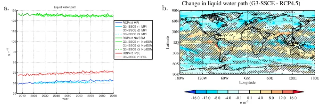
[21] Changes in cloud liquid water path (LWP) may be
viewed as a measure of the second indirect effect (lifetime effect), and we therefore in Figure 4a show the time evolution of this quantity. We note that in all three models, LWP remains approximately constant in time throughout the G3-SSCE simulations. In the RCP4.5 simulations, on the other hand, LWP increases slightly with time in IPSL-CM5A and MPI-ESM, as might be expected in a warming climate, but remains unchanged in NorESM, which has a weaker warming.
The fact that the LWP changes in IPSL-CM5A and MPI-ESM are very similar even though the IPSL-CM5A does not account for the second indirect effect at all suggests that in a globally averaged sense, cloud changes are more influenced by climate change than by in situ cloud microphysical effects. 3.2. Changes in TOA Radiative Fluxes and the
Hydrological Cycle
[22] We will now turn to global distributions of the
multimodel mean changes due to G3-SSCE. Figure 5 shows the change in TOA net (down minus up)fluxes of longwave (LW) (Figure 5a), SW (Figure 5b), and total (LW + SW) (Figure 5c) radiation over the 2060s. The overall positive values of net LW radiation (Figure 5a) are due to lower emissions in a colder climate, as discussed in connection with Figure 1a above, but we note that there are significant geographical variations. The models agree on the sign of the change over most land surfaces, while there are some Figure 4. (a) As in Figure 1a but for liquid water path (g m 2). (b) As in Figure 2b but for liquid water
path (g m 2).
Figure 5. As in Figure 2b but for (a) TOA net LW radiation (W m 2, down minus up), (b) TOA net SW
radiation (W m 2, down minus up), (c) TOA net SW + LW radiation (W m 2, down minus up), and (d) clear-sky TOA net SW radiation (W m 2, down minus up).
discrepancies over ocean, especially in the storm-track regions. It turns out that the low-latitude land regions that experience the largest increases in net LW flux, i.e. the largest decrease in OLR (Figure 5a), also experience an increase in the cloud cover across all models (Figure 6a). Inevitably, for the net SW radiation, based on the design of the G3-SSCE experiments, there is a distinct band of strongly negative values in the marine sea-salt injection region from 30°S to 30°N where the models also agree on the sign of the change (Figure 5b). In addition, a consistent decrease in net SW radiation is also visible over land regions such as the African continent, large parts of Asia south of 45°N, and Australia.
[23] To understand these changes, we note that these
low-latitude land regions experience an increase in cloud cover (Figure 6a), which increases the reflected solar radiation. Looking back at net LW radiation, wefind positive values in those same regions, which is also consistent with the increase in cloud amount. Together, these three factors (net LW radiation, net SW radiation, and cloud cover changes) illustrate a kind of “Walker circulation effect” as follows: The immediate effect of G3-SSCE is to reduce the absorption of solar radiation at the low-latitude ocean surface, while the adjacent land regions are unaffected. As a response to that, a low-latitude circulation is induced with sinking motion over ocean and rising motion over land. This circulation is superimposed on the preexisting low-latitude atmospheric circulation. The rising motion over land enhances the con-vection there, leading to more cloudiness, including high clouds, causing a distinct decrease in the net SW radiation and a corresponding increase in the net LW radiation. This
is illustrated by Figure 7, which displays the difference in low-latitude vertical motions between G3-SSCE and RCP4.5. We note the negative values, corresponding to enhanced rising motion or weakened sinking motion over longitudes corresponding to the land masses of Africa and the Arabian peninsula (10°W to 50°E in the Northern Hemisphere (NH), 20°E to 40°E in the Southern Hemi-sphere (SH)), Oceania and Indonesia (110°E to 180°E in SH), Central and South America (95°–115°W in NH and 40°–70°W in SH), and East Asia (80°E to 120°E in NH), whereas there are positive values over the Atlantic Ocean (15–35°W) and parts of the Pacific Ocean between 160°E and 90°W. The Walker circulation effect is also highlighted in Table 2, which gives the changes in various parameters separately over land and ocean. As the table shows, the net TOA radiation change is positive over land, while it is negative over ocean, mainly due to a strong suppression of OLR over land. We also note that LHF, which over ocean is reduced by almost 4 W m 2, is almost unchanged over
land between the two simulations. As a result, precipitation is marginally increased over land, despite the colder geo-engineered climate, whereas over ocean where the cooling is less pronounced, the precipitation reduction is an order of magnitude larger than over land (Table 2).
[24] In the storm-track regions, all the models obtain an
increase in downwelling SW radiation (Figure 5b) due to the reduced cloud cover in these regions (Figure 6a). The re-duced cloud cover is probably due to a weakening of the mid-latitude storm tracks as a result of a reduced pole-to-equator temperature gradient caused by the spatial pattern of total TOAflux change seen in Figure 5c. The weakening of the Figure 6. (a) As in Figure 2b but for cloud cover (%). (b–d) Zonally averaged difference in cloud cover
(%) between simulations G3-SSCE and RCP4.5 averaged over the time period 2060–2069 for IPSL-CM5A, MPI-ESM, and NorESM, respectively.
storm tracks is evidenced by a weakening of the subtropical jet streams in both hemispheres (not shown).
[25] The change in TOA net flux between the G3-SSCE
experiments and RCP4.5 is negative over most of the oceanic seeding region (Figure 5c), and all three models agree on the sign of this change. One region that stands out with particu-larly large changes in SW (Figure 5b) and net (Figure 5c) radiation is the west coast of northern South America, with an associated extension along the equator from 75°W to 120°W. We note from Figure 6a that these changes cannot be understood from cloud cover changes alone, but as shown in Figure 4b, there is a particularly large increase in LWP in this area. Closer inspection (not shown) indicates that the NorESM has very high sea-salt concentrations and CDNC changes in this area, due to a combination of converging winds (especially along the equator) and persistent low clouds (especially along the coast of South America). These changes are then fed into the other models, as discussed in section 2, and it turns out that the signal seen in Figure 5c has a particularly large contribution from the MPI-ESM, which has persistent, susceptible clouds in this area (not shown). The fact that LWP responds so strongly to sea-salt injections is a manifestation of the lifetime effect, as in both the MPI-ESM and the NorESM precipitation release is influenced by cloud droplet size and hence CDNC.
[26] Outside the seeding region, there are compensating
positive values, and all three models agree on an increase in net radiation over the northern part of Africa, the Middle East, the Gobi desert, and Australia. While these regions are affected by the increase in cloud cover (Figure 6a) in both the SW and the LW, the high surface albedo in these semiarid regions makes the contribution from changes in cloud cover on the SW radiation small compared to the LW effect, and the resulting change in net radiation is positive. The same effect of the surface albedo on the net TOAflux is found over Antarctica (Figure 5c).
[27] As mentioned in section 1, SSCE operates both
through enhanced cloudy-sky solar reflectance (MCB or “indirect effect”) and through enhanced clear-sky solar reflectance (“direct effect”). In order to assess the relative contributions of these two effects, we show in Figure 5d the clear-sky change in TOA net SWflux. Comparing this figure
to Figure 5b, we see a much smoother image, as the clear-sky effect is insensitive to the spatially inhomogeneous cloud distribution. However, in areas with persistent clouds, such as in the aforementioned region off the west coast of South America and along the equatorial eastern Pacific, the cloudy-sky contribution dominates. As shown in Table 2, on average the clear-sky contribution at low latitudes is 69%, with the remaining 31% coming from cloudy sky.
[28] Figure 6a shows the multimodel mean change in
frac-tional cloud cover, while the average global, land area, and ocean area changes in cloud cover are listed in Table 3. From this overview we see that on average the cloud cover increases in G3-SSCE compared to RCP4.5, the increase in percent cloud cover being 0.08 over ocean and 0.36 over land regions. Figure 6a shows that the models agree on the sign of the change over northern Africa, Asia south of 45°N, much of Australia, and in the storm-track regions, while the response differs in sign elsewhere.
[29] In order to relate the cloud changes to TOA radiative
fluxes, it is not sufficient to consider total cloud cover, which is a two-dimensional field obtained from cloud fraction at individual model levels, combined with an assumption on cloud overlap. More insight can be gained by studying changes
a) b)
Figure 7. Vertical west-east cross sections showing the difference in omega-vertical velocity (in 103hPa s 1) between G3-SSCE and RCP4.5 for the time period 2060–2069, averaged over the latitude bands (a) 10°–35°N and (b) 10°–35°S.
Table 2. Changes Due to Climate Engineering (G3-SSCE Minus RCP4.5) of Selected Key Parameters Averaged Over the Three Models, Averaged Over Low Latitudes (Between 35°S and 35°N), and Separately Over Land and Oceana
Total Land Ocean Net downwardflux, TOA (W m 2) 1.08 0.94 1.80 Outgoing LW radiation (W m 2) 1.69 2.74 1.32 Outgoing SW radiation (W m 2) 2.78 1.80 3.12 Total cloud cover (%) 0.35 0.85 0.17 Precipitation (mm day 1) 0.07 0.01 0.10 Near-surface air temperature (K) 0.75 0.92 0.69 Water vapor path (kg m 2) 2.06 1.53 2.24 Surface upward latent heatflux (W m 2) 2.80 0.11 3.76 Surface upward sensible heatflux (W m 2) 0.13 1.11 0.21 Liquid water path (g m 2) 0.07 0.36 0.04 Outgoing SW radiation, clear sky (W m 2) 1.91 0.93 2.25 Outgoing SW radiation, cloudy sky (W m 2) 0.87 0.87 0.87
in the vertical distribution of clouds, and in Figures 6b–6d we show this quantity for each of the three models. Starting with the IPSL-CM5A model, which in Andrews et al. [2012] was found to exhibit a very pronounced positive cloud feedback, we see (Figure 6b) that in the cooler G3-SSCE climate, compared to RCP4.5, there is a pronounced downward shift in upper-tropospheric cloudiness as the tropical tropopause is lowered in a cooler climate [cf. Lorenz and de Weaver, 2007]. This downward shift and the associated increase in cloud top temperature leads to a significant suppression of the clouds’ ability to trap infrared radiation [e.g., Zelinka et al., 2012]. Low-latitude boundary layer clouds, on the other hand, are found to increase in areal extent. Both these changes tend to enhance the cooling of the climate, which the G3-SSCE forcing is already cooling. In the MPI-ESM model (Figure 6c), the cloud changes bear resemblance to those in the IPSL-CM5A model, while in NorESM (Figure 6d) the upper-tropospheric changes are much weaker than in the other two models, possi-bly due to lower vertical resolution in NorESM. Importantly, in NorESM, the low-level cloudiness is decreased in the colder G3-SSCE climate, implying a suppression of the reflectance
of solar radiation, thereby reducing the cooling effect of the climate engineering. To a significant extent, these changes explain the significantly smaller G3-SSCE-induced cooling in NorESM than in the IPSL-CM5A and MPI-ESM models noted above, in connection with Figure 2a.
[30] Figure 8a shows the difference in latent heat flux
between G3-SSCE and RCP4.5. We note that the suppres-sion of the latent heatflux previously mentioned in connection with Figure 3a is largely confined to the low-latitude ocean regions, where the G3-SSCE is implemented. This is in agree-ment with the MCB experiagree-ments of Bala et al. [2011]. In agreement with the enhanced net radiation over low-latitude land regions in Figure 5c, wefind in Figure 8a a significant increase in the latent heatflux over many low-latitude land regions, such as Australia, northern Africa, and the Arabian Peninsula, while there are slight reductions over Indonesia, the Amazonas, and central Africa. For sensible heat flux (Figure 8b), the opposite is found, i.e., a general suppression over low-latitude land areas, and a slight but consistent increase over the oceans. The tendency for many land regions to exhibit higher latent heatfluxes and lower sensible heat fluxes in the engineered climate indicates an enhanced avail-ability of water at the surface, i.e., reduced aridity. This can also be clearly seen by looking at changes in the Bowen ratio (Figure 8c), defined as SHF/LHF, which is a good measure of aridity. Whereas the latent heat flux dominates over wet surfaces, in increasingly dry soil conditions, the sensible heat becomes more and more dominant [Fischer et al., 2007]. Figure 8c shows reduced Bowen ratios over many land regions equatorward of 40° latitude, while at higher latitudes the values are generally small.
[31] The G3-SSCE-induced change in vertically integrated
water vapor path, also referred to as precipitable water, is shown in Figure 8d. There is a general reduction in the mass
Table 3. As in Table 2, Except Globally Averaged
Global Land Ocean Net downwardflux, TOA (W m 2) 0.45 0.87 1.00 Outgoing LW radiation (W m 2) 1.39 2.01 1.13 Outgoing SW radiation (W m 2) 1.84 1.14 2.13 Total cloud cover (%) 0.16 0.36 0.08 Precipitation (mm day 1) 0.06 0.02 0.08 Near-surface air temperature (K) 0.66 0.82 0.59 Water vapor path (kg m 2) 1.43 1.03 1.59 Surface upward latent heatflux (W m 2) 1.86 0.29 2.51 Surface upward sensible heatflux (W m 2) 0.12 0.50 0.37 Liquid water path (g m 2) 1.36 1.21 1.42
Figure 8. As in Figure 2b but for (a) latent heatflux at the surface (W m 2, positive upward), (b) sensible
heatflux at the surface (W m 2, positive upward), and (c) Bowen ratio (nondimensional). Grey areas indicate undefined values. (d) Water vapor path (percentwise change).
of water vapor, as expected in a colder climate, and the reduc-tion is strongest around the Intertropical Convergence Zone (ITCZ), where it amounts to 5–10%. This reduction in ITCZ water vapor is caused by reduced evaporation over the low-latitude oceans due to weaker solar radiation (Figure 8a) and weaker trade winds (not shown), weakening the low-latitude transport of moisture toward the ITCZ. Consequently, the ITCZ has significantly suppressed precip-itation (Figure 9a), whereas the nearby trade wind regions have, if anything, a slight tendency for enhanced precipita-tion. The only regions with intermodel-consistent increases (0–5%) in water vapor path are found over parts of the Antarctic, possibly associated with changes in the Southern Hemisphere storm tracks.
[32] In agreement with the changes in the low-latitude
circulation (Figure 7) and the discussion thereof, we find enhanced precipitation over northern Africa, Australia, the Arabian Peninsula, and northern India, all of which also show positive anomalies in latent heatflux (Figure 8a) and water vapor path (Figure 8d). High-latitude continents have a consistent but rather weak reduction in precipitation, and the same is the case for the storm track regions, in agreement with the reduction in cloud cover noted earlier (Figure 6a).
[33] Investigating precipitation changes in individual
sea-sons, wefind in June-July-August (JJA) increased precipita-tion over most of the Indian subcontinent, related to the Indian summer monsoon (Figure 9b). In northern Africa, summertime precipitation is likewise increased, in particular over the Sahelian region, but there is a reduction in JJA precipitation over many ocean regions at 0–10°N, as well
as over northern South America. Increased precipitation is found in all seasons over Australia, most consistently in the southern provinces (not shown). All seasons except December-January-February show an increased precipitation in southern Europe and a reduction in northern Europe, extending eastward into Siberia.
3.3. Termination Effect
[34] The last 20 years of the simulations, beyond the
50 years of CE, allow us to study the consequences of abruptly shutting off the CE, referred to as the termination effect. Figure 10a shows that from the last decade of SSCE (2060s) the near-surface temperature increased worldwide across all models with a particularly strong signal in the Arctic exceeding 2 K within 20 years after CE was turned off (2080s). Globally averaged, this increase reached 0.7 K (Table 4). This rapid warming brings the globally averaged near-surface temperature to RCP4.5 levels within 10 to 15 years of terminating the SSCE (Figure 2a). Figure 10b shows that the precipitation decreases over many low-latitude continental regions during the same period, with models agreeing over northern Africa, the Middle East, and parts of Australia. There is also model agreement on an increase in precipitation over North America, northern Europe, and Siberia. As for temperature, the globally averaged precipitation reaches RCP4.5 levels within 10 to 15 years (Figure 3c). Jones et al. [2013] studied the termination effect of the GeoMIP G2 experiment in which the forcing from an annual 1% increase in CO2concentration was canceled by reducing the solar
constant. The geographical pattern of change in near-surface Figure 9. Simulated difference in precipitation (mm day 1) between simulations G3-SSCE and RCP4.5,
both averaged over the time period 2060–2069. Hatching denotes areas where the three models disagree on the sign of the change. (a) Annually averaged change. (b) Seasonal change averaged over June-July-August.
Figure 10. Termination effect. Simulated differences between G3-SSCE simulations averaged over the time period 2080–2089 minus the time period 2060–2069. Hatching denotes areas where the three models disagree on the sign of the change. (a) Near-surface temperature (K). (b) Precipitation (mm day 1).
air temperature and its intermodel consensus of our study (Figure 10a) are in agreement with thefindings of the G2 termination effect study. The rapid increase in global pre-cipitation following termination (Figure 3c) and the general model agreement of precipitation increases at midlatitudes and high latitudes (Figure 10b) are also found by Jones et al. [2013]. Unlike the findings of our study, however, the global surface temperature and precipitation did not reach non-geoengineered levels within 20 years of termination in the G2 experiment.
[35] Figure 11 shows that the Arctic September multimodel
sea ice fraction decreased regionally by over 25% when turn-ing off the SSCE. This substantial decrease in ice cover explains the Arctic amplification in the termination effect temperature signal, also in agreement with Jones et al. [2013].
4. Summary and Conclusions
[36] Using three state-of-the-art Earth system models, we
have studied multidecadal simulations of 21st century climate evolution for two cases: an RCP4.5 pathway and climate engi-neering simulations using sea-salt injections over low-latitude oceans to maintain a constant TOA radiative forcing for 50 years, followed by a termination of the climate engineering (G3-SSCE). To our knowledge, this is thefirst multimodel study of climate engineering through sea-salt injections.
[37] The results show that on a global scale, sufficiently
large SSCE leads to a cancelation of the warming seen in RCP4.5 in all the models. The experimental strategy of keep-ing the forckeep-ing at 2020 levels is responsible for a continued global temperature increase the first 15–20 years of G3-SSCE as the climate system is not yet in equilibrium. This is seen in results from the IPSL-CM5A and the NorESM, while global temperature stabilization occurs much faster in the MPI-ESM. The MPI-ESM has pronounced trends in some quantities throughout G3-SSCE, e.g., gradually increasing OSR and decreasing OLR and decreasing latent heat flux and precipitation, while the IPSL-CM5A and the NorESM do not show trends in these quantities.
[38] Despite significant differences in simulated climate
response between the models, e.g., very different cloud feed-backs and different susceptibilities to sea-salt injections, all three modelsfind a suppression of latent heat flux and precip-itation over the low-latitude oceans, which are being subjected to negative radiative forcing through sea-salt climate engineer-ing. Conversely, over the low-latitude continents all three
models find an enhanced latent heat flux and increase in cloud cover as well as precipitation and a reduction in aridity as evidenced by widespread reductions in the Bowen ratio. Together, these land-ocean changes represent an impor-tant shift in the hydrological cycle that can be viewed as an “enhanced Walker circulation”. In this regard, our study confirms the robustness of the results from the earlier sin-gle-model study of Bala et al. [2011]. By comparison, the GeoMIP G1 study by Schmidt et al. [2012] found suppressed precipitation over both low-latitude land and ocean regions, and the desert brightening study by Bala and Nag [2011] found low-latitude land-sea changes that were opposite to those found here. The results of these three studies are phys-ically consistent since at low latitudes a significant portion of the precipitation is caused by moist convection from an un-derlying surface heated by solar radiation.
[39] Over the low-latitude oceans, many spatial features of
the results can be attributed to a cloud lifetime effect associ-ated with sea-salt injections. This effect is simulassoci-ated in two of the three models, and it is manifested through enhanced LWP and, to a lesser extent, cloud cover enhancements in areas of persistent and susceptible low clouds, e.g., along the west coast of Peru. A consequence of this effect is a strong enhancement of reflected solar radiation. Nevertheless, a partitioning of TOA radiation changes into cloudy-sky and clear-sky contributions yields the largest contribution from clear sky, even over low-latitude oceans where MCB might be expected to dominate. This suggests that at least in the three models considered here, low-latitude marine sea-salt injections may act more strongly via clear-sky direct effect than MCB. A similar result was found for the Goddard Institute for Space Studies ModelE2 Earth System Model by Kravitz et al. [2013], whereas Jones and Haywood [2012] using the HadGEM2 ES Earth System Model and Partanen et al. [2012] using ECHAM5.5-HAM2 climate-aerosol model found the indirect effect resulting from MCB to dominate over the direct effect. More studies are needed to clarify the reasons for these intermodel differences.
Table 4. Changes Due to Termination of Climate Engineering for Selected Key Parameters Averaged Over the Three Models, Globally Averaged, and Separately Over Land and Oceana
Global Land Ocean Net downwardflux, TOA (W m 2) 0.55 0.77 1.09 Outgoing LW radiation (W m 2) 1.48 2.13 1.21 Outgoing SW radiation (W m 2) 2.03 1.37 2.31 Total cloud cover (%) 0.06 0.33 0.05 Precipitation (mm day 1) 0.07 0.03 0.09 Near-surface temperature (K) 0.73 0.92 0.66 Water vapor path (kg m 2) 1.50 1.09 1.67 Surface upward latent heatflux (W m 2) 2.01 0.51 2.63 Surface upward sensible heatflux (W m 2) 0.09 0.67 0.40 Liquid water path (g m 2) 1.20 0.90 1.32
aG3-SSCE 2080s minus 2060s.
Figure 11. Termination effect. Simulated September dif-ferences in fractional sea ice cover between G3-SSCE simu-lations averaged over all three models for the time period 2080–2089 minus the time period 2060–2069.
[40] Due to, e.g., differences in cloud feedback, we find
significant differences between the models in the amplitude of the low-latitude changes. The IPSL-CM5A has a strong positive cloud feedback, because in the cooler geoengineered climate, there is an enhancement of low-level cloudiness and a pronounced downward shift in upper level cloudiness, both of which cool the climate further. In NorESM, the cloud feedback is negative, and a suppression of geoengineered cooling is found, while the MPI-ESM results are somewhere in between the IPSL-CM5A and the NorESM.
[41] The termination effect is manifested through a
world-wide rapid increase in near-surface temperature with a partic-ularly large increase in the Arctic exceeding 2 K within 20 years after CE has ceased, in agreement with Jones et al. [2013]. This Arctic amplification is caused by a substantial decrease in the September Arctic sea ice fraction of over 25% regionally. All models show that most variables reach RCP4.5 values within 10 to 15 years after CE shutoff.
[42] The planned GeoMIP experiments of marine cloud
brightening [Kravitz et al., 2013] will allow a large set of models to participate in coordinated experiments and will fur-ther test the robustness of thefindings in this work, in addition to expanding our overall knowledge of this CE technique.
[43] Acknowledgments. This study was partly funded by the European Commission’s 7th Framework Program through the IMPLICC project (FP7-ENV-2008-1-226567) and the EuTRACE project (grant 306395). J.E.K. and K.A. received support from the Norwegian Research Council through the EarthClim project (207711/E10) and its program for supercomputing (NOTUR) through a grant of computing time. H.S., U.N., and C.T. are thank-ful to the MPI-ESM development team and the DKRZ where MPI-ESM simulations have been performed and archived. The IPSL-CM5A climate sim-ulations were performed with the HPC resources of [CCRT/TGCC/CINES/ IDRIS] under the allocation 2012-t2012012201 made by GENCI (Grand Equipement National de Calcul Intensif ), CEA (Commissariat à l’Energie Atomique et aux Energies Alternatives), and CNRS (Centre National de la Recherche Scientifique).
References
Albrecht, B. (1989), Aerosols, cloud microphysics, and fractional cloudi-ness, Science, 245, 1227–1230.
Alterskjær, K., and J. E. Kristjánsson (2013), The sign of the radiative forcing from marine cloud brightening depends on both particle size and emission amount, Geophys. Res. Lett., 40, 210–215, doi:10.1029/2012GL054286. Alterskjær, K., J. E. Kristjánsson, and Ø. Seland (2012), Sensitivity to
delib-erate sea salt seeding of marine clouds—Observations and model simula-tions, Atmos. Chem. Phys., 12, 2795–2807.
Andrews, T., J. M. Gregory, M. J. Webb, and K. E. Taylor (2012), Forcing, feedbacks and climate sensitivity in CMIP5 coupled atmosphere-ocean climate models, Geophys. Res. Lett., 39, L09712, doi:10.1029/2012/ GL051607.
Bala, G., and B. Nag (2011), Albedo enhancement over land to counteract global warming: Impacts on hydrological cycle, Clim. Dyn., 37, doi:10.1007/ s00382-011-1256-1.
Bala, G., P. B. Duffy, and K. E. Taylor (2008), Impact of geoengineering schemes on the global hydrological cycle, Proc. Natl. Acad. Sci. U.S.A., 105, 7664–7669.
Bala, G., K. Caldeira, R. Nemani, L. Cao, G. Ban-Weiss, and H.-J. Shin (2011), Albedo enhancement of marine clouds to counteract global warming: Impacts on the hydrological cycle, Clim. Dyn., 37, 915–931, doi:10.1007/s00382-010-0868-1.
Baughman, E., A. Gnanadesikan, A. Degaetano, and A. Adcroft (2012), Investigation of the surface and circulation impacts of cloud-brightening geoengineering, J. Clim., 25, 7527–7543, doi:10.1175/JCLI-D-11-00282.1.
Bentsen, M., et al. (2013), The Norwegian Earth System Model, NorESM1-M—Part 1: Description and basic evaluation, Geosci. Model. Dev., 6, 687–720.
Coumou, D., and S. Rahmstorf (2012), A decade of weather extremes, Nat. Clim. Change, doi:10.1038/nclimate1452.
Crutzen, P. (2006), Albedo enhancement by stratospheric sulfur injec-tions: A contribution to resolve a policy dilemma?, Clim. Change, 77, 211–219.
Dufresne, J.-L., et al. (2013), Climate change projections using the IPSL-CM5 Earth System Model: From CMIP3 to CMIP5, Clim. Dyn., 40, 2123–2165, doi:10.1007/s00382-012-1636-1.
Fischer, E. M., S. I. Seneviratne, P. L. Vidale, D. Lüthi, and C. Schär (2007), Soil moisture–Atmosphere interactions during the 2003 European summer heat wave, J. Clim., 20, 5081–5099.
Giorgetta, M. A., et al. (2013), Climate and carbon cycle changes from 1850 to 2100 in MPI-ESM simulations for the Coupled Model Intercomparison Project 5, JAMES, 5, 572–597.
Gregory, J. M., W. J. Ingram, M. A. Palmer, G. S. Jones, P. A. Stott, R. B. Thorpe, J. A. Lowe, T. C. Johns, and K. D. Williams (2004), A new method for diagnosing radiative forcing and climate sensitivity, Geophys. Res. Lett., 310, L03205, doi:10.1029/2003GL018747. Hill, S., and Y. Ming (2012), Nonlinear climate response to regional
bright-ening of tropical marine stratocumulus, Geophys. Res. Lett., 39, L15707, doi:10.1029/2012GL052064.
Jones, A., and J. M. Haywood (2012), Sea-spray geoengineering in the HadGEM2-ES Earth-system model: Radiative impact and climate response, Atmos. Chem. Phys., 12, 10,887–10,898, doi:10.5194/acp-12-10887-2012.
Jones, A., J. Haywood, and O. Boucher (2009), Climate impacts of geoengineering marine stratocumulus clouds, J. Geophys. Res., 114, D10106, doi:10.1029/2008JD011450.
Jones, A., et al. (2013), The impact of abrupt suspension of solar radiation management (termination effect) in experiment G2 of the Geoengineering Model Intercomparison Project (GeoMIP), J. Geophys. Res. Atmos., 118, 9743–9752, doi:10.1002/jgrd.50762.
Korhonen, H., K. S. Carslaw, and S. Romakkaniemi (2010), Enhancement of marine cloud albedo via controlled sea spray injections: A global model study of the influence of emission rates, microphysics and transport, Atmos. Chem. Phys., 10, 4133–4143.
Kravitz, B., A. Robock, O. Boucher, H. Schmidt, K. E. Taylor, G. Stenchikov, and M. Schulz (2011), The Geoengineering Model Intercomparison Project (GeoMIP), Atmos. Sci. Lett., 12, 162–167.
Kravitz, B., et al. (2013), Marine cloud brightening experiments in the Geoengineering Model Intercomparison Project (GeoMIP): Experiment design and preliminary results, J. Geophys. Res. Atmos., 118, 11,175–11,186, doi:10.1002/jgrd.50856.
Latham, J. (1990), Control of global warming?, Nature, 347, 339–340. Latham, J., P. Rasch, C.-C. Chen, L. Kettlers, A. Gadian, A. Gettelman,
H. Morrison, K. Bower, and T. Choularton (2008), Global tempera-ture stabilization via controlled albedo enhancement of low-level mar-itime clouds, Philos. Trans. R. Soc., 366, 3969–3987, doi:10.1098/ rsta.2008.0137.
Lorenz, D. J., and E. T. de Weaver (2007), Tropopause height and zonal wind response to global warming in the IPCC scenario integrations, J. Geophys. Res., 112, D10119, doi:10.1029/2006JD008087.
Moss, R. H., et al. (2010), The next generation of scenarios for climate change research and assessment, Nature, 463, 747–756, doi:10.1038/ nature08823.
Partanen, A.-I., H. Kokkola, S. Romakkaniemi, V.-M. Kerminen, K. E. J. Lehtinen, T. Bergman, A. Arola, and H. Korhonen (2012), Direct and indirect effects of sea spray geoengineering and the role of injected par-ticle size, J. Geophys. Res., 117, D02203, doi:10.1029/2011JD016428. Rasch, P., J. Latham, and C.-C. J. Chen (2009), Geoengineering by cloud
seeding: Influence on sea ice and climate system, Environ. Res. Lett., 4, doi:10.1088/1748-9326/4/4/045112.
Rogelj, J., J. Nabel, C. Chen, W. Hare, K. Markmann, M. Meinshausen, M. Schaeffer, K. Macey, and N. Hohne (2010), Copenhagen Accord pledges are paltry, Nature, 464, 1126–1128.
Salter, S., G. Sortino, and J. Latham (2008), Sea-going hardware for the cloud albedo method of reversing global warming, Philos. Trans. R. Soc., 366, 3989–4006, doi:10.1098/rsta.2008.0136.
Schmidt, H., et al. (2012), Solar irradiance reduction to counteract radiative forcing from a quadrupling of CO2: Climate responses simulated by four
Earth system models, Earth Syst. Dyn., 3, 63–78.
Twomey, S. (1977), The influence of pollution on the shortwave albedo of clouds, J. Atmos. Sci., 34, 1149–1152.
Zelinka, M. D., S. A. Klein, and D. L. Hartmann (2012), Computing and partitioning cloud feedbacks using cloud property histograms. Part II: Attribution to changes in cloud amount, altitude, and optical depth, J. Clim., 25, 3736–3754.