SEARCH FOR EXTRASOLAR PLANETS THROUGH HIGH CONTRAST DIFFRACTION LIMITED INTEGRAL FIELD SPECTROSCOPY

(1)

HAL Id: tel-00580958

https://tel.archives-ouvertes.fr/tel-00580958

Submitted on 29 Mar 2011

HAL is a multi-disciplinary open access

archive for the deposit and dissemination of sci-entific research documents, whether they are pub-lished or not. The documents may come from teaching and research institutions in France or abroad, or from public or private research centers.

L’archive ouverte pluridisciplinaire HAL, est destinée au dépôt et à la diffusion de documents scientifiques de niveau recherche, publiés ou non, émanant des établissements d’enseignement et de recherche français ou étrangers, des laboratoires publics ou privés.

SEARCH FOR EXTRASOLAR PLANETS THROUGH

HIGH CONTRAST DIFFRACTION LIMITED

INTEGRAL FIELD SPECTROSCOPY

Jacopo Antichi, Kjetil Dohlen

To cite this version:

Jacopo Antichi, Kjetil Dohlen. SEARCH FOR EXTRASOLAR PLANETS THROUGH HIGH CON-TRAST DIFFRACTION LIMITED INTEGRAL FIELD SPECTROSCOPY. Astrophysics [astro-ph]. Università degli studi di Padova, 2007. English. �tel-00580958�

(2)

SEARCH FOR EXTRASOLAR PLANETS

THROUGH HIGH CONTRAST

DIFFRACTION LIMITED

INTEGRAL FIELD SPECTROSCOPY

Jacopo Antichi

Department of Astronomy

University of Padova

Thesis submitted towards the degree of

Doctor of Philosophy

(3)

(4)

UNIVERSITÀ DEGLI STUDI DI PADOVA, DIPARTIMENTO DI ASTRONOMIA

Coordinatore: Ch.mo Prof. Giampaolo Piotto

Relatori: Dott. Raffaele Gratton, INAF-Osservatorio Astronomico di Padova Dott. Massimo Turatto, INAF-Osservatorio Astronomico di Padova

Controrelatore: Dr. Kjetil Dohlen, Laboratoire d'Astrophysique de Marseille & Observatoire Astronomique de Marseille Provence

(5)

(6)

Subject

This Dissertation is devoted to high contrast diffraction limited Integral Field Spectroscopy for the direct imaging of extrasolar planets. The aim is to describe this subject in the domain of signals dominated by Speckles residual. This latter being the specific working case of the Integral Field Spectrograph (IFS) planned for the next Planet Finder instrument of the Very Large Telescope facility (SPHERE). In the effort of realizing the Integral Field Unit of this instrument, we found a new optical concept (BIGRE) allows to overcome all the features affecting the Slit Functions of a 3D-Spectrograph working in this optical regime. As a consequence, the proposed IFS is a complete BIGRE oriented instrument, optimized for the SPHERE system. More generally, the presented theory on diffraction limited Integral Field Spectroscopy is largely new and could contribute in advancing the field of high contrast imaging.

(7)

(8)

Summary

Nowadays the extrasolar planet research can be raised to the level of a new chapter of Astrophysics, combining different domains of science: Physics of sub-stellar objects, Planetology, Astrobiology and Optics in an interdisciplinary way; in this sense, this matter “rides the wave” of the evolutive epoch we are leaving, the one of the interdisciplinary information.

The statistics on the properties of planets and their parent stars is increasing monthly, and is opening the way to the next step of this research, the direct detection. The first direct detection of a stellar companion with a planetary mass, occurred only in 2004, when distinct images of a star 2M1207 and of its low-mass companion were finally obtained, exploiting a few among the best astronomical facilities available today: VLT/NACO and HST/NICMOS. After the first detection, the ones of GQ Lup b and AB Pictoris b followed in 2005. However, these cases should be considered the first pioneering efforts to try to collect separately the light of a planet from the one of the parent star and, at present, it remains a non-standard technique in Astronomy.

Direct detection techniques, such the ones based on high contrast imaging or interferometry, could overcome the limits of the in-direct approaches. The Transit technique - for instance - provides the radius of a low-mass companion only. Derivation of the planet mass by the periodic variation of the stellar light curve is impossible unless Radial Velocity measures are available: the object may be a planet, but also a low mass star or a brown dwarf or a white dwarf, whose radii are similar to the Earth one. The Radial Velocity technique - in turn - is sensitive only to extrasolar planets with relatively small orbits, typically corresponding to objects at a distance smaller than a few AU from their parent star, or with high eccentricity. These limitations lead to ambiguous interpretations on the properties of what has been actually detected, biasing both single-object and statistical analyses.

Simultaneous Differential Imaging (SDI) is a high contrast differential calibration technique, allowing to create several images taken at different wavelengths of the same field of view around a target star. Subtraction of simultaneous monochromatic images is a way to remove the Speckle Noise which dominates over any other optical pattern inside the angular separation boundary, where a suitable Adaptive Optics system restores the diffraction limit fixed by the telescope aperture. This calibration technique has produced already a number of important scientific results in the realm of sub-stellar objects, reaching star vs. planet Contrast of order of 104-105 with the NACO-SDI facility at the VLT. Presently, the Contrast threshold allowing to detect (young) Jupiter-like planets - around 107 - is the challenge for the next ground based Planet Finder projects as the European one SPHERE.

SPHERE will mount the first Integral Field Spectrograph aimed to the direct detection of extrasolar planets. The theory joining 3D-Spectroscopy and extrasolar planets direct detection represents what, in this Dissertation, we defined as Spectroscopical Simultaneous Differential Imaging (S-SDI). In this frame, diffraction limited Integral field Spectroscopy is needed to obtain monochromatic images over the entire field of view around a target star. Then, through 3D-Spectroscopy, simultaneous difference of monochromatic images should exceed the standard Simultaneous Differential Imaging, based on chromatic filters only. The work presented in this Dissertation is entirely devoted to high contrast diffraction limited Integral Field Spectroscopy. The aim is to describe this subject, leading the reader to

(9)

approaching step by step the domain of diffraction limited Integral Field Spectroscopy, from the ideal case, up to the real case of a Speckle dominated input signal. This latter being the specific case of the SPHERE Integral Field Spectrograph (IFS). Design of a diffraction limited IFS requires careful consideration of a number of subtle effects, including not uniform illumination of the entrance aperture (causing diffraction patterns different from the classical Airy disk), cross talk between adjacent spaxels (i.e. pixels in the spatial dimension) caused by the wings of the diffraction profiles, and correct sampling in both spatial coordinates and wavelength. Appropriate consideration of these effects should be combined in a design where the largest field of view, spectral resolution and coverage are obtained at the cheapest possible cost (this being mainly driven by the number of detector pixels).

In the effort of realizing the Integral Field Unit of this instrument, we found that a new optical concept - BIGRE - allows to overcome all the features affecting the Slit Functions of a 3D-Spectrograph working in this optical regime. As a consequence, the SPHERE Integral Field Spectrograph presented in this Dissertation is a complete BIGRE oriented instrument. The theory of a diffraction limited IFS presented in this Dissertation is largely new, and it is the most important original contribution of this work.

Finally, this Dissertation ends describing the contribution we gave for the 3D-Spectroscopy facility foreseen within the EPICS instrument. EPICS is a feasibility study for a Planet Finder for the OWL Telescope promoted by ESO in 2005. It was based on a collaboration of expertises from all over Europe; the design explored different possible frameworks for the future European ELT.

The structure of the Dissertation is as follows: in Section 1 we introduce the topic of extrasolar planet research; special emphasis is given to the model atmosphere for extrasolar giant planets, on which both Simultaneous Differential Imaging and the Spectroscopical Simultaneous Differential Imaging achieve their scientific reasons. Section 2 is dedicated to a panoramic description of the detection methods useful to the search for planets; here special emphasis is given in the comparison between direct and in-direct detection methods. The fact that in-direct detection method will remain fundamental even after direct detection techniques will be operative is clearly stated. In Section 3 Simultaneous Differential Imaging and Spectroscopical Simultaneous Differential Imaging are defined, described and compared. The important aspect here is that - in principle - S-SDI is much powerful that the standard SDI, and that the Integral Field Spectrograph of SPHERE could reach Constrast values as high as 107, i.e. the (young) Jupiter Contrast size. In Section 4 the SPHERE project is described as a whole, except for the Integral Field Spectrograph. Sections 5 and 6 are fully dedicated to this subject. Specifically, Section 5 is dedicated to the general description of the classical TIGER and the new BIGRE devices, and to the optimization of the BIGRE Integral Field Unit of this Integral Field Spectrograph. Results of laboratory prototyping are presented; they confirm that BIGRE is the right optical solution in order to achieve the science goals of this Integral Field Spectrograph. Section 6 describes the IFS optical design, and Section 7 finally, the work we did for the 3D-Spectroscopy channel foreseen for EPICS.

(10)

Sommario

La ricerca di pianeti extrasolari oggi può essere considerata come un nuovo capitolo della Astrofisica che riunisce differenti campi scientifici: Fisica degli oggetti sub-stellari, Planetologia, Astrobiologia ed Ottica in modo interdisciplinare; in questo senso questa materia “cavalca l’onda” dell’epoca in cui viviamo, quella della conoscenza interdisciplinare.

L’inferenza statistica riguardante le proprietà dei pianeti e delle loro stelle ospiti migliora di mese in mese e sta aprendo la strada per il passo successivo di questa ricerca, la rivelazione tramite metodi diretti. La prima scoperta diretta di un compagno stellare di massa planetaria è avvenuta solo nel 2004, quando, finalmente, sono state ottenute immagini distinte della stella 2M1207 e del suo compagno di piccola massa, usufruendo di un paio dei migliori strumenti per l’Astronomia disponibili oggi: VLT/NACO e HST/NICMOS. Dopo questo primo ritrovamento, nel 2005 sono seguiti quelli di GQ Lup b ed AB Pictoris b. Tuttavia, questi casi devono essere considerati come esempi pionieristici dell’intento di rappresentare separatamente la luce di un pianeta e quella della sua stella madre. Al momento, in Astronomia questi casi rimangono esempi di rivelazione non standardizzati in una tecnica consolidata.

Le tecniche per la scoperta diretta, come quelle basate sull’Imaging ad alto contrasto o l’Interferometria, possono superare i limiti propri degli approcci indiretti. La tecnica dei Transiti - per esempio - fornisce come informazione fisica solo il raggio del compagno di piccola massa. Ricavare la massa del pianeta attraverso la variazione periodica della curva di luce della stella ospite è impossibile a meno che siano disponibili anche misure di Velocità Radiale: l’oggetto in questione potrebbe essere un pianeta ma anche una stella di piccola massa, oppure una nana bruna od una nana bianca, il cui raggio è simile a quello della Terra. A sua volta, la tecnica delle Velocità Radiali è sensibile alla presenza di un pianeta, nel caso in cui esso abbia orbita relativamente stretta - tipicamente essa corrisponde ad oggetti con distanza più piccola di qualche UA dalla stella madre -, oppure nel caso in cui la sua orbita abbia un valore di eccentricità alto. Questi limiti comportano interpretazioni ambigue su ciò che effettivamente è stato rivelato, pregiudicando l’analisi sul singolo oggetto, come quella sull’intero campione statistico.

L’Imaging Differenziale Simultaneo (SDI) è una tecnica di calibrazione differenziale ad alto contrasto che permette di creare alcune immagini di diversa lunghezze d’onda e dello stesso campo di vista attorno ad una stella target. La sottrazione simultanea di immagini monocromatiche è utilizzata come metodo per rimuovere il rumore di Speckle. Esso domina su ogni altro “pattern ottico” compreso nell’intervallo di separazione angolare dove un sistema di Ottica Adattiva opportuno restaura il limite ottico di diffrazione, fissato a sua volta dall’apertura del telescopio. Questa tecnica di calibrazione ha già prodotto importanti risultati scientifici nel regno degli oggetti sub-stellari, arrivando a valori di Contrasto stella vs. pianeta dell’ordine di 104-105 con lo strumento NACO-SDI al VLT. Al momento, la soglia di Contrasto che permette di rivelare pianeti gioviani (giovani) - dell’ordine di 107 - rappresenta la sfida per i prossimi progetti da terra per la rivelazione diretta dei pianeti extrasolari, tra cui quello Europeo SPHERE.

SPHERE monterà il primo Spettrografo a Campo Integrale indirizzato alla rivelazione diretta di pianeti extrasolari. La teoria che collega Spettroscopia 3D e la rivelazione diretta di pianeti extrasolari è ciò che, in questa Dissertazione, noi definiamo come Imaging Differenziale Simultaneo Spettroscopico (S-SDI). In questa prospettiva, la Spettroscopia a

(11)

Campo Integrale al limite ottico di diffrazione è necessaria per ottenere immagini sull’intero campo di vista attorno ad una stella target. Poi, sempre attraverso la Spettroscopia 3D, la differenza simultanea di immagini monocromatiche dovrebbe superare l’Imaging Differenziale Simultaneo standard, che è basato solo su filtri cromatici.

Il lavoro qui presentato è interamente dedicato alla Spettroscopia a Campo Integrale al limite ottico di diffrazione in condizione di alto contrasto. La volontà è di descrivere questo argomento, portando il lettore ad avvicinarsi passo dopo passo al domino della Spettroscopia a Campo Integrale al limite ottico di diffrazione, partendo dal caso ideale, fino al caso reale di un segnale di ingresso dominato dal rumore di Speckle. Specificamente, quest’ultimo è il caso in cui opererà lo Spettrografo a Campo Integrale montato su SPHERE. La progettazione di uno Spettrografo a Campo Integrale ottimizzato per lavorare al limite ottico di diffrazione richiede di fare attenzione a fenomeni ottici complessi, ad esempio l’illuminazione non uniforme delle fenditure di ingresso (questo causa profili di diffrazione diversi dal classico disco di Airy), cross talk tra spaxel adiacenti (cioè pixel nella dimensione spaziale) causato dalle ali dei profili di diffrazione, ed il corretto campionamento del segnale di ingresso sia nelle coordinate spaziali che in lunghezza d’onda. L’esame opportuno di questi effetti deve essere combinato in un progetto ottico dove il massimo campo di vista e la giusta risoluzione spettrale siano ottenute con il minimo costo possibile (quest’ultimo dipende principalmente dal numero di pixel del rivelatore).

Nell’intento di realizzare l’Unità a Campo Integrale di questo strumento, abbiamo messo a punto un nuovo concetto ottico - BIGRE - che permette di superare tutti gli effetti che intaccano le Funzioni di Fenditura di uno Spettrografo 3D, operante in questa condizione ottica. Come conseguenza, lo Spettrografo a Campo Integrale di SPHERE, presentato in questa Dissertazione, è completamente orientato al concetto ottico BIGRE. La teoria di uno uno Spettrografo a Campo Integrale ottimizzato per lavorare al limite ottico di diffrazione è in gran parte nuova e rappresenta il contributo originale più importante di questo lavoro. Infine, questa Dissertazione termina con la descrizione del contributo che abbiamo dato alla realizzazione dello Spettrografo 3D previsto all’interno dello strumento EPICS. EPICS è uno studio di fattibilità per un Planet Finder - adatto al Telescopio OWL - promosso da ESO nel 2005. Questo lavoro si è basato sulla collaborazione di esperti provenienti da tutta Europa; nella progettazione si sono esplorati possibili adattamenti per il futuro Extremely Large Telescope Europeo.

La struttura di questa Dissertazione è la seguente: nella Sezione 1 introduciamo l’argomento dei pianeti extrasolari; è data particolare enfasi ai modelli di atmosfera relativi ai pianeti extrasolari giganti, sui quali sia l’Imaging Differenziale Simultaneo e l’Imaging Differenziale Simultaneo Spettroscopico traggono la loro ragione scientifica. La Sezione 2 è dedicata ad una descrizione panoramica dei metodi utili nella rivelazione dei pianeti extrasolari; particolarmente sottolineata è la comparazione tra metodi diretti e metodi indiretti. E’ spiegato chiaramente il fatto che i metodi indiretti rimarrano fondamentali una volta che le tecniche di detezione diretta saranno operative. Nella Sezione 3 sono definite, descritte e comparate le tecniche di Imaging Differenziale Simultaneo ed Imaging Differenziale Simultaneo Spettroscopico. Il fatto importante qui è che - di principio - la tecnica S-SDI è più potente della tecnica SDI standard, e che lo Spettrografo a Campo Integrale di SPHERE è in grado di raggiungere valori di Contrasto dell’ordine di 107_{, cioè i}

valori di Contrasto tipici dei pianeti gioviani (giovani). Nella Sezione 4 è descritto l’intero progetto SPHERE, eccetto lo Spettrografo a Campo Integrale. Le Sezioni 5 a 6 sono completamente dedicate a questo argomento. Specificamente, la Sezione 5 riguarda la descrizione generale del classico dispositivo TIGER e del nuovo dispositivo BIGRE, e

(12)

l’ottimizzazione della Unità a Campo Integrale di questo Spettrografo 3D. Inoltre, sono presentati i risultati del prototipo di laboratorio; essi confermano che BIGRE è la soluzione ottica vincente per soddisfare il caso scientifico di questo strumento. La Sezione 6 ne descrive il disegno ottico e la Sezione 7 - infine - presenta il lavoro svolto per il canale di Spettroscopia 3D previsto per EPICS.

(13)

(14)

List of Figures

Figure 1-1: Central temperature as a function of age for different masses. TH ,TLi and TD

indicate the hydrogen, lithium and deuterium burning temperatures, respectively (cfr.

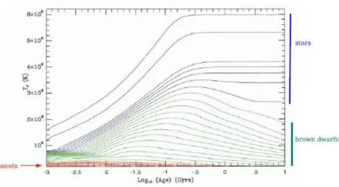
Chabrier and Baraffe 2000). 35 Figure 1-2: Theoretical evolution of the central temperature for stars, brown dwarfs and

planets from 0.3 MJUPITER to 0.2 MSUN. Notice the increase (Maxwell-Bolzmann

plasma), maximum and decrease (Fermi-Dirac plasma) of the central temperature for brown dwarfs. The red lines indicate sub-stellar objects with mass lower than 12 x 10-3 MSUN that represents the sharpest criterion in distinguishing planets and brown dwarfs

(cfr. Burrows et al. 2001). 36 Figure 1-3: Example of observed M and L dwarf spectra in the range 0.5-2.5 [micron] from

M9 to L 5.5. SDSS or 2MASS identifications are given above the dashed line that corresponds to the zero flux level for each spectrum (cfr. Geballe et al. 2002). 38 Figure 1-4: Example of observed L dwarf spectra in the range 0.5-2.5 [micron] from L 6.5 to

L 9.5. SDSS or 2MASS identifications are given above the dashed line that corresponds

to the zero flux level for each spectrum (cfr. Geballe et al. 2002). 38 Figure 1-5: Example of observed T dwarf spectra in the range 0.5-2.5 [micron] from T 0 to T

4.5. SDSS or 2MASS identifications are given above the dashed line that corresponds

to the zero flux level for each spectrum (cfr. Geballe et al. 2002). 38 Figure 1-6: Example of observed T dwarf spectra in the range 0.5-2.5 [micron] from T 4.5 to

T 8. SDSS or 2MASS identifications are given above the dashed line that corresponds

to the zero flux level for each spectrum (cfr. Geballe et al. 2002). 39 Figure 1-7: Dependence of a model of dwarf spectrum on the vertical extent of the

condensate cloud. A sharper cloud-top cut off - parameterized by the scalar s1 and by

the size of the single cloud particle a0 - results in a bluer infrared spectrum (cfr.

Burrows et al. 2006). 40 Figure 1-8: Companions (M2) mass function of the Sun-like stars closer than 25 pc, plotted

against mass (cfr. Grether and Lineweaver 2006). 41 Figure 1-9: The faint part of the I vs. (I-J) colour-magnitude diagram for the Pleiades. Points

represent field stars, while the large filled circles are the confirmed brown dwarfs cluster population (indicated as redder than the dash colour-magnitude boundary). Triangles represent known field brown dwarfs, shifted to the distance of the cluster. The solid line and the dash-dotted line represent respectively the ~120 [Myr] DUSTY isochrones (Chabrier et al. 2000) and the ~125 [Myr] NextGen isochrones (Baraffe et al. 1998), shifted to the distance of the cluster. Finally, upper and the lower dotted lines at the bottom of the diagram indicate the completeness and limiting magnitude of the

survey (cfr. Bihain et al. 2006). 43 Figure 1-10: The derived mass function for the Pleiades (cfr. Bihain et al. 2006). Filled

circles are cumulative data obtained by the counts of the observed brown dwarf population and open circles are the data points obtained by Deacon and Hambly (2004). The solid line - over imposed to the data points - represents the log-normal mass function obtained by Deacon and Hambly (2004), normalized to the total number of object in this survey between 0.5 MSUN down to the completeness mass limit of this

(19)

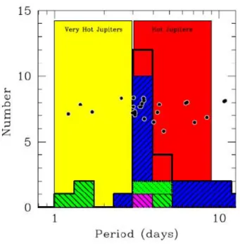
Figure 1-11: Period distribution of the short period extrasolar giant planets. The blue shaded histogram shows planets with mass M sin(i) > 0.2 MJUPITER detected via Radial

Velocities surveys, the green-shaded histogram shows planets detected via OGLE-TRansit surveys and magenta shaded histogram shows the planet detected via the TrES survey. The yellow and the red bands indicate the fiducial period ranges of the Very-Hot-Jupiter and the Very-Hot-Jupiters, while the black points show the individual periods of

the planets (cfr. Gaudi et al. 2005). 46 Figure 1-12: Emergent spectrum of a class I (Teq~130 K, cfr. Sudarsky et al. 2003) extrasolar

giant planet placed at 10 pc from the Earth. 48 Figure 1-13: Emergent spectrum of a class II (Teq~200 K, cfr. Sudarsky et al. 2003)

extrasolar giant planet placed at 10 pc from the Earth. 49 Figure 1-14: Emergent spectrum of a class III (Teq~500 K, cfr. Sudarsky et al. 2003)

extrasolar giant planet placed at 10 pc from the Earth. 49 Figure 1-15: Emergent spectrum of a class IV (Teq~1000 K, cfr. Sudarsky et al. 2003)

extrasolar giant planet placed at 10 pc from the Earth. 49 Figure 1-16: Emergent spectrum of a class V (Teq~1500 K, cfr. Sudarsky et al. 2003)

extrasolar giant planet placed at 10 pc from the Earth. 50 Figure 1-17: Spectral albedo of photosynthetic (green), non-photosyntetic (dry) vegetations

and the Earth’s soil according to Clark (1999). 51 Figure 1-18: Spectral albedo of the Earth as determined by the Earthshine measure of Woolf

et al. (2002), with a model spectrum super-imposed. This latter is the sum of the various contributions as the Figure shows. The interferometric pattern on the right-center of the Figure is the CCD fringing by which the instrumental spectrum produced by the

detector was divided. 52 Figure 1-19: Earthshine contributing area of the Earth during the observation of

Montanez-Rodriguez et al. (2005) (2003 November 19-th, 10.47-13.08 UT hour). The super-imposed colour map represents the mean cloud distribution form the ISCCP data over

this area. 52 Figure 1-20: Histogram of Minimum Mass for 167 known extrasolar planets found with

M⋅sin(i)<15 MJ (cfr. Butler et al. 2006). 53

Figure 1-21: Histogram of the semi-major orbital axis distribution for the 104 planets found in the uniform Doppler survey (accuracy ~3 [m⋅sec-1_{]) of 1330 star conducted by the}

Lick, Keck, Anglo-Australian telescopes with a duration of ~8 [yr] (cfr. Marcy et al.

2005). 54 Figure 1-22: Eccentricity vs. semi-major orbital axis distribution for the 104 planets in the

sample of Marcy et al. (2005). 54 Figure 1-23: M⋅sin(i) vs. semi-major orbital axis distribution for the 104 planets in the

sample of Marcy et al. (2005). 55 Figure 1-24: Orbital eccentricity vs. M⋅sin(i) distribution for the 104 planets in the sample of

Marcy et al. (2005). 55 Figure 1-25: Frequency of extrasolar planets in bins of different metallicity in the sample of

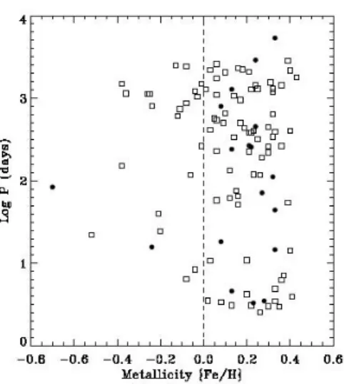
Marcy et al. (2005). 56 Figure 1-26: Occurrence of Very-Hot-Jupiters vs. metallicity in the sample (cfr. Sozzetti

(20)

Figure 1-27: 24 [micron] Spitzer/MIPS images of three protoplanetary disks around high mass O type stars (NGC 2244, NGC2264, IC 1396) together with a model image for the

tail in NGC 2244 (upper right panel), cfr. Balog et al. 2006. 59 Figure 1-28: Montage of resolved dusty disk around mains sequence stars in ascending order

from left to right, top to bottom (from Augereau et al. 2004). The 3 top panels display disks seen is scattered light using coronagraphic techniques to mask the central bright

star. The 3 bottom panels display disks seen in IR and FIR emitted light. 60 Figure 2-1: Comparison between the flux emitted by the Sun (a G2V star) and those coming

from the planets of the Solar System (J=Jupiter, V=Venus, E=Earth, M=Mars). Z represents the spectral distribution of the zodiacal light. The two peaks in the VIS-NIR-MIR correspond to the maxima of reflected light and intrinsic emission respectively

(from Vérinaud et al. 2006). 68 Figure 2-2: Main features in the VISible-Near IR spectra of the most important molecules

expected to be present in planetary atmospheres (H2O, O2, O3, CH4, CO2, N2O), from

Traub and Jucks (2002) and Des Marais et al. (2002). 69 Figure 2-3: Detection methods for extrasolar planets. The lower extent of the lines indicates,

roughly, the detectable masses that are in principle within reach of present measurements (solid lines), and those that might be expected within the next 10-20 [yr] (dashed). The (logarithmic) mass scale is shown at left. The miscellaneous signatures to the upper right are less well quantified in mass terms. Solid arrows indicate (original) detections according to approximate mass, while open arrows indicate further measurements of previously-detected systems. ‘?’ indicates uncertain or unconfirmed

detections (cfr. Perryman 2000). 70 Figure 2-4: Orbital parameters of a planet-star system. In this Figure, the star (s) and the

planet (p) are assumed to be in circular orbit around the center of mass (cm) of the system (more in general, the orbit would be elliptical). The orbital radii are as for the

star and ap for the planet. These are plotted along the orbital plane. The orbital

inclination angle (i) between the normal to the orbital plane and the line of sight determines the orbital inclination angle. The Radial Velocity Vs of the star as measured

along the line of sight (from the upper right in the diagram) depends on the sine of the

orbital inclination angle. 71 Figure 2-5: Radial Velocity signal of the star 51 Pegasi as measured with SARG. 71

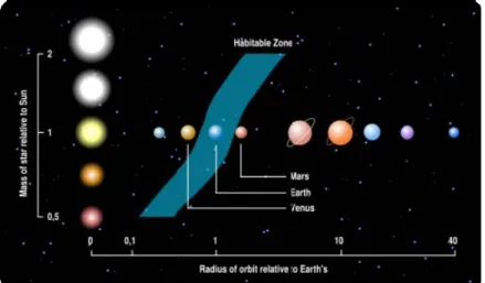
Figure 2-6: Habitable Zone distance and width vs. mass of the hosting star expressed in

MSUN unit. 73

Figure 2-7: Astrometry Variation (α) induced on the parent star for the known planetary systems, as a function of orbital period. Circles are shown with a radius proportional to MP⋅sin (i). Astrometry at the milliarcsec level has negligible power in detecting these

systems, while the situation changes dramatically for microarcsec measurements. Effects of Earth, Jupiter, and Saturn are shown at the distances indicated. The Gaia detection limit is also shown, from ESA/ESO report on extrasolar planets: Perryman et

al. (2005). 74 Figure 2-8: Schematic representation of a transiting planet across the stellar disk. The planet

is shown from first to fourth contact. The stellar flux (solid line) diminishes by ∆F during a Transit for a total time of tT while tF is the duration between to instants of the

Transit called respectively Ingress and Egress. The curvature seen on the light curve during Transit is consequence of the star limb darkening of the stellar disk. The impact

(21)

parameter (b) is shown also in term of the orbital inclination angle (i) and the orbital

semi-major axis (a). Finally the stellar radius is indicated as RS. 76

Figure 2-9: Masses and radii for 9 transiting planets as well as Jupiter and Saturn. Dashed lines represent the radius vs. mass relation parameterized in term of the planets density

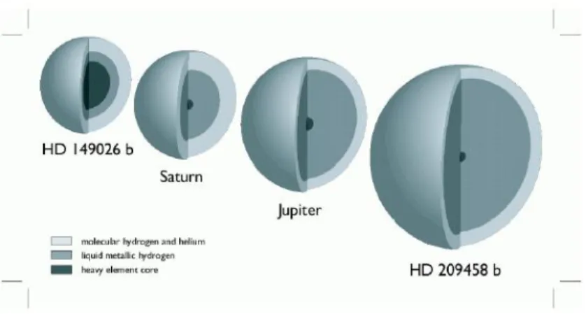
(ρ), cfr. Charbonneau et al. (2006). 77 Figure 2-10: Cut-away diagram of Jupiter, Saturn, the two exotic Hot-Jupiters (HD 209458 b

and HD 149026 b) drawn to scale. The observed radius of HD 149026 b implies a massive core of heavy elements making perhaps 70% of the planetary mass. In contrast, the radius of HD 209458 b would indicate a coreless structural model or an additional

energy source to explain its large value, cfr. Charbonneau et al. (2006). 78 Figure 2-11: Diagnostic diagram for the evaporation status of extrasolar planets. 182

identified planets are plotted with symbols depending on the spectral type of the central star: triangles for F type, filled circles for G type, diamonds for K type and squares for M type. The absence of planets below the line for which the Radial Velocity signal is lower than 10 [m⋅sec-1_{] indicates a selection effect. While, the lifetime line at t}

2=5 [Gyr]

shows that there are no detected Hot-Jupiters in this part of the diagram because this is

a forbidden evaporation region, cfr. Lecavelier des Etangs (2006). 78 Figure 2-12: HST photometric light-curves of the Transit of TrES-1 (top) and HD 209458 b

(bottom). The shorter orbital period and the smaller size of the TrES-1 star result in a Transit that is shorter in duration than that of HD 209458 b. Similarly, the smaller star creates a deeper Transit for TrES-1, despite the fact that HD 209458 b gets a larger radius. TrES-1 light-curve shows a light-hump centred a time of -0.01 days from the light-curve minimum. This is likely the result of the planet occulting a star-spot on the

stellar surface (cfr, Charbonneau et al. 2006). 81 Figure 2-13: (Top) data and best fit model for the OGLE-2005-BLG-169 event. (Bottom) the

difference between this model and the classical form of a single-lens pattern. The

extrapolated mass of the planet is ~13 MEARTH, cfr. Gould et al. (2006). 82

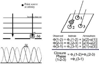
Figure 2-14: Differential Phase technique explained through the Young’s two-slit experiment (cfr. Born and Wolf 1965). The presence of a planet causes a phase shift in

the stellar fringe observed by a long-baseline optical interferometer. 86 Figure 2-15: In an interferometer, a phase delay above an aperture causes a phase shift in the

detected fringe pattern (left panel). Phase errors introduced at any telescope causes equal but opposite phase shifts, cancelling out in the closure phase (right panel).

Equations on the right panel are taken from Readhead et al. (1988). 88 Figure 2-16: Mass vs. separation diagram illustrating the complementarities of different

techniques used for extrasolar planet direct detection. The black circles indicate known planets discovered through in-direct methods. The shaded regions show the approximate parameter space accessible to direct detection techniques employing

Interferometry and high contrast imaging, from Beuzit et al. (2006). 89 Figure 2-17: An H-band image from one of best coronagraphic devices in the world today:

the Lyot Project Coronagraph. This instrument is an optimized, diffraction limited, classical Coronagraph (i.e. Lyot-like) fitted behind an AO system with Control Radius =10 [cm] on the 3.67 [m] AEOS telescope on Mahui islands, currently the highest order AO correction available (cfr. Oppenheimer et al. 2004). The companion (confirmed through common proper motion Astrometry) to this nearby star gets a Contrast of 10-4.5

(22)

Figure 3-1: Spectra (flux densities in [mJy]) of 5 MJUPITER planets with log10 Age: 8.5, 9.0,

9.5 and 9.7 [yr] (from top to bottom). The effective temperatures span between ~200-600 K and the wavelength range is 0.7-1.8 [micron]. From models of Burrows et al.

(2003). 98 Figure 3-2: Parent-to-star flux ratio from 0.5 to 6.0 [micron] for a MJUPITER planet orbiting a

G2V star at 4 AU as a function of the planet age: 0.1, 0.3, 1.3 and 5 [Gyr], from

Burrows et al. (2004). 99 Figure 3-3: Parent-to-star flux ratio from 0.5 to 6.0 [micron] for a 5 [Gyr] planet orbiting a

G2V star at 4 AU as a function of the planet mass: 0.5, 1, 2, 4, 6, and 8 MJUPITER, from

Burrows et al. (2004). 99 Figure 3-4: NIR spectrum of a G2V star sampled with to different spectral steps

corresponding to R=15 (solid line) and R=375 (dotted line). The plot does not include the telluric absorptions proper of the wavelengths range 0.8-1.8 [micron]. Notice the featureless profile of this stellar spectrum at different spectral resolutions. By courtesy

of the CHEOPS team. 99 Figure 3-5: Simulation of the Contrast (5σ detection threshold) vs. separation to the center

for a G2V star a 5 pc in 4 hours observing time, efficiency 0.3, and spectral step equal to λ/50 without Speckle Noise subtraction: in this case a relation scale is valid over all the wavelength bands up to the M one. Curves are computed in different wavelengths band below the K-band limit with realistic SR levels for the AO-compensation of the

signal coming from this model star (by courtesy of the CHEOPS team). 100 Figure 3-6: Simulation of the Contrast (5σ detection threshold) vs. separation to the center

for the same star of Figure 3-5 with Speckle Noise subtraction: in this case it comes clear that Sky Noise dominate L’ and M bands and that the achievable Contrast vs. separation is nearly flat. Curves are computed in different wavelength windows below the K-band with realistic SR levels for the AO-compensation of the signal coming from

this model star (by courtesy of the CHEOPS team). 101 Figure 3-7: Short-exposure (0.1 sec) natural (left) and AO-compensated (right) images of a

star obtained with the CFHT “bonnette” AO-system at λ=1.6 [micron] and D/r0~4. The

grey scale is logarithmic in intensity (from Racine et al. 1999). Notice that the increasing Speckle brightness toward the PSF center and the appearance of the bright

diffraction limited core with size ~2λ/D. 105 Figure 3-8: Quasi-static Speckle pattern. The images show the high spatial frequency content

of long exposures taken with NACO at the VLT separated by about one hour (from

Vérinaud et al. 2006). 105 Figure 3-9: Example of adopted phase screen in the Speckle Noise simulator Code described

in Berton et al. (2006), by courtesy of the CHEOPS team. At left: a phase screen produced by software CAOS (cfr. Carbillet et al. 2004) representing a perturbed wavefront not corrected by Adaptive Optics. At right: the same phase screen

AO-compensated. 107 Figure 3-10: Example of simulated Speckle pattern with coronagraphic spatial filtering of

the coherent part of the central PSF with the Speckle Noise simulator Code described in Berton et al. (2006), by courtesy of the CHEOPS team. The object is a G0V star, the Entrance Pupil size is 8 m and its shape is proper of a VLT telescope in the Nasmyth configuration, the integration time is 0.5 [sec] and the adopted Entrance Pupil phase

(23)

Figure 3-11: Comparison between the speckle noise (dash-dotted line), the photon noise (dashed line), and the noise in the differential image (solid line) obtained using the Speckle Noise simulator Code described in Berton et al. (2006) - by courtesy of the CHEOPS team - as a function of separation for a simulated G0V star at 3 pc from Earth. The ratio between the Speckle and Photon Noises is 102. Notice that the simulations considered in the preparation of this figure assume a Speckle patter field due to

atmospheric turbulence only. 108 Figure 3-12: A 3D-view of NACO-SDI optical design, by courtesy the CHEOPS team. The

double Wollaston Prism separates the beam coming from the AO-Camera Focal Plane in 4 parts. Then, the Camera re-images the Focal Plane of the telescope on 4 distinct 1024 x 1024 array detectors. Before the focus, a 4Q chromatic narrow-band filter is

inserted to obtain simultaneous images in 3 different wavelengths. 111 Figure 3-13: Raw images on the focus of NACO-SDI, by courtesy of the CHEOPS team.

The simultaneous difference between them strongly attenuates the Speckle Noise. 111 Figure 3-14: Optical sketch of the TRIDENT Camera mounted at CFHT and OMM. After

the Lyot Stop, the beam separator uses a combination of 2 polarizing beam splitters, 2 right-angle Prisms, and a first order quarter-wave retarder to generate 3 optical beams, each one organized in a “L”-shape reproducing - as a whole - the shape of a trident. 112 Figure 3-15: Schematic comparison of three Integral Field Spectrograph concept: Image

Slicer Spectrograph (a), TIGER-type Spectrograph (b), FTS (c), from Vérinaud et al.

(2006). 115 Figure 3-16: The principle of an Image Slicer. The slicer mirror array, located on the

re-imaged telescope Focal Plane, divides the FOV and re-images the telescope Exit Pupils along a line on the pupil mirrors. Each pupil mirror then re-images its corresponding slice of the FOV on its corresponding slit mirror located at the Spectrograph Focal Plane. The re-formatted FOV acts as the Entrance Slit in the Spectrograph where all the

slices are aligned as a pseudo long slit (cfr. Prieto and Vivès 2006). 116 Figure 3-17: The TIGER optical concept as reduced by Lee et al. (2001). The IFS Entrance

Slit Plane becomes a matrix of micro-pupils corresponding to different parts of the

original FOV. 116 Figure 3-18: Spectral plot for the light feeding a spaxel near the position θ of a simulated

Jovian planet. The modulation induced on the intrinsic spectrum by the Speckle

Chromatism is clearly visible (from Sparks and Ford 2002). 117 Figure 3-19: Cuts through the original data cube with one spatial dimension (horizontal axis)

and one spectral dimension (vertical axis). In the original cube (top panel) the rings diverge outward with wavelength, while in the spatially re-sampled cube (bottom panel), they form a straight lines running vertically in the plot (from Sparks and Ford

2002). 118 Figure 3-20: Model of a NIR spectrum in the range 0.80-1.80 [micron] of a 1 MJUPITER planet

orbiting a solar-type star (G2V) which is 1 [Gyr] old, with a separation of 10 AU. The spectral emission is mainly intrinsic, with a negligible component of reflected light. The solid spectrum has a spectral resolution R=15 while the dotted one R=375, from Berton

et al. (2006). 119 Figure 3-21: Model f a NIR spectrum of the same planet of Figure 3-20, but at separation of

(24)

reflected light. The solid spectrum has still a spectral resolution R=15 and the dotted

one R=375, from Berton et al. (2006). 120 Figure 3-22: Final output of an IFS observation of a star in the case of the Entrance Pupil

proper to the VLT Nasmyth configuration. Top-left: example of telescope PSF before AO-compensation and Coronagraph spatial filtering, after the simulation of the TIGER-type IFU and the disperser, a large image is obtained. Bottom left: details of the spectra. Separations are expressed in [arcsec]. The spectral range is 0.95-1.70 [micron] and the spectral resolution R=15, so the length of a single spectrum is about 20 pixels (from

Berton et al. 2006). 120 Figure 3-23: Rebuilt monochromatic image obtained using the DRSW of Berton et al.

(2006). As explained in the text, from the spectra of Figure 3-22, a set of images such

as this are obtained before SDI procedure. 121 Figure 3-24: Results of the simultaneous difference operated after a correct chromatic

re-scaling of the monochromatic images. A brown dwarf of 30 MJUPITER finally arises from

the Noise (S/N=30), on the top of this simulated image (from Berton et al. 2006). 121 Figure 3-25: The H-band spectrum of GQ Lup b compared to the spectra of L0 dwarfs of

different ages. The peaked continuum shape of the spectrum of GQ Lup b strongly resembles to that of ~10 [Myr] old 2MASS J01415823-4633574, indicating similarity in low surface gravity and spectral type. All the spectra are normalized to unity at 1.68

[micron], (cfr. McElwain et al. (2006). 122 Figure 4-1: Global concept of the SPHERE instrument indicating its 4 sub-systems:

Common Path, ZIMPOL, IRDIS and IFS. It also includes the main functionalities within the Common Path sub-system. Optical beams are red for NIR, blue for VISible

and orange for Common Path. 127 Figure 4-2: Implementation of SPHERE on the VLT Nasmyth platform 127

Figure 4-3: Sketch of the SAXO loop structure. 128 Figure 4-4: Prototype of the HWP proper to the 4QPMC proposed by the SPHERE team

(from Mawet et al. 2006). 129 Figure 4-5: Experimental and simulated PSF profiles obtained with the 4QPMC proposed by

the SPHERE team. The grey solid curve is the reference experimental PSF in the range 0.7-1.0 [micron]. The continuous black line is the experimental post-Coronagraph PSF profile. The dashed line is the result of simulations taking into account of the waveplates phase residuals and de-focus errors. For comparison, the simulations result obtained with a monochromatic mask - used in the same conditions - is shown by the

dotted curve (from Mawet et al. 2006). 130 Figure 4-6: Basic polarimetric principle of ZIMPOL. 130

Figure 4-7: Current optical design of ZIMPOL. 131 Figure 4-8: Current optical design of IRDIS. 132 Figure 4-9: Block diagram for the SPHERE performances simulator Code. Modules are

distinguished only for common procedures. The module “focal-plane 2” represents the performances simulator Code implemented - respectively - for ZIMPOL, IRDIS and

IFS. 133 Figure 5-1: Profile of IFS Slit Function (solid line) of the single re-imaged WHT Entrance

(25)

The dashed line represents the fit obtained with three (dotted lines) Gaussian functions

(from Bacon et al. 2001). 135 Figure 5-2: Optical concept of a TIGER IFU: the IFS Slits Plane is filled with an array of

micro-images of the telescope Entrance Pupil. 136 Figure 5-3: Simulated profile of a monochromatic IFS Slit Function @ λ=1.35 [micron] in

the case of the TIGER spaxel. Normalization is done with respect to the central value and the ordinate scale is logarithmic. The adopted Output Focal Ratio is FOUT=8. 138

Figure 5-4: TIGER spaxel in a nutshell. 138 Figure 5-5: Optical concept of a BIGRE IFU: the IFS Slits Plane is filled with an array of

micro-images of the telescope Focal Plane. 139 Figure 5-6: Simulated profile of a monochromatic IFS Slit Function @ λ=1.35 [micron] in

the case of the BIGRE spaxel. Normalization is done with respect to the central value and the ordinate scale is logarithmic. The adopted spaxel Output Focal Ratio is

FOUT=8.13 and DSPM=30.72 [mm]. 141

Figure 5-7: BIGRE spaxel in a nutshell. 141 Figure 5-8: Example of simulated bi-dimensional screen (0.5 [msec] integration time),

generated by the SPHERE performance simulator (see Section 4.4). It represents the expected input to the SPHERE Integral Field Unit (by courtesy of the SPHERE team).

144 Figure 5-9: 2D-image of the Slits Functions simulated by the VLT-PF team. The shape of the single TIGER spaxel is square, producing the SINC2_{profile proper the FT of a}

square aperture. Strong distortions due to this effect are clearly visible; the color scale

is logarithmic: blue is hot, red is cold. 144 Figure 5-10: Image of the MicroPupils Plane of the simulated TIGER IFU adopted by the

CHEOPS team. The shape of the single spaxel is circular, producing an Airy Pattern profile. The modulation of the FT of the residual Speckle pattern field on the shape of the single MicroPupils is quite small, and only Intensity variations among re-imaged telescope Entrance Pupils are clearly visible in this 2D-screen. The color scale is

logarithmic: white is hot, grey is cold. 145 Figure 5-11: Distribution of the intensities within the 2 central pixels (dpixel=18 [micron]) of

the IFS Slit Function profile resulting from a simulation of the TIGER IFU optimized by the CHEOPS team. The imposed Output Focal Ratio is FOUT=8. Any Intensity value

is normalized to the total Intensity incident on the single spaxel; the acquisition time is 4 [hr]. All the spaxels produce a SF central-peak whose Intensity is very close to that given by a Uniform Illumination i.e. the Airy Pattern proper to a circular aperture with size equal to the one of the single spaxel. Overimposed a Gaussian curve that fits the

obtained statistical distribution with RMS=4.2x10-5. 145 Figure 5-12: Images of the IFS Slits obtained with the BIGRE IFU, at the OAPD/Lab. The

Shape Distortion of the Slit Functions is practically absent and only Intensity variations among different IFS Slits remain. The color scale is logarithmic: white is hot, grey is

cold. 146 Figure 5-13: Cuts through the data cube obtained by the chromatical dispersion of the IFS

Slits resulting from the prototype TIGER IFU simulated by the VLT-PF team. The spatial dimension is on the horizontal axis, while the spectral dimension is on the vertical axis. The red and blue lines indicate two spectra taken at different radial

(26)

distances to the optical axis. Moving along these spectra, a variable pseudo-periodic

modulation - depending on the wavelength - is clearly visible. 146 Figure 5-14: Sketch of the final spectra (black rectangles) superimposed on an array of 7

(red) hexagonal spaxels, inside of a lenses-based IFU. In this picture, Coherent CrossTalk is the interference signal between monochromatic IFS Slits corresponding to adjacent lenses i.e. separated by a distance equal to DL; while Incoherent CrossTalk is

the spurious signal registered over a fixed monochromatic IFS Slit and due to its

adjacent spectra. 149 Figure 5-15: Possible spectra alignment for the Square configuration of lens based IFU. The

reference axis is aligned to a side of the square. Notice that the symmetries of a square configuration allow to analyze only alignments having Position Angles < α ≤ π/4. 153 Figure 5-16: Possible spectra alignment for the Hexagonal configuration of a lens based IFU.

The reference axis is aligned to a side of the hexagon. Notice that the symmetries of a hexagonal lens based IFU allow to analyze only configurations having Position Angles

α ≤ π/6. 153 Figure 5-17: Example of spectra alignment: the considered case in the Hexagonal-B (cfr.

Table 5-1). 154 Figure 5-18: Estimate of the CCT (~10-2.25 at 150 [micron]) and ICT (~10-3.5 at 75 [micron])

for the same Slit Function shown in Figure 5-3. Normalization is done with respect to the central value and the ordinate scale is logarithmic. These values are not sufficient

for reaching the SPHERE/IFS Contrast goal of C>107_{. 156}

Figure 5-19: Estimate of the CCT (~10-3_{at 150 [micron]) and ICT (~10}-6_{at 75 [micron]) for}

the same Slit Function shown in Figure 5-6. Normalization is done with respect to the central value and the ordinate scale is logarithmic. The values are sufficient (Coherent CrossTalk) or well beyond (Incoherent CrossTalk) the limits allowing to reach the

SPHERE/IFS Contrast goal of C>107. 157

Figure 5-20: Optical design of the BIGRE IFU to be mounted on SPHERE/IFS. 158 Figure 5-21: Viewgraph of the spreadsheet by which the BIGRE solution for the

SPHERE/IFU system has been obtained. The checks at the bottom (colored in green) consider all the constraints imposed by the SPHERE/IFS TLRs and the Technical Constraints inside the SPHERE main module. Notice that the spreadsheet contains - as

Outputs - the basic specifications of the SPHERE/IFS optical design. 159 Figure 5-22: Optical design of a single BIGRE lens for the prototyping of SPHERE/IFU. 160

Figure 5-23: Photo-image of the adopted IFU prototype realized by microoptic systems

gmbh . 161

Figure 5-24: Microscope-image of a portion of the prototype IFU. The deposited mask, that

renders the shape of first surface of the lenses circular, is clearly visible. 161 Figure 5-25: Autocorrelation of the microscope-image of the prototype IFU. 161 Figure 5-26: Optical design of the 3D-Spectrograph adopted for the prototyping. The red

arrow indicates the position of the Spectrograph Pupil Mask. 162 Figure 5-27: CCD-image of the IFS Slits Plane obtained with the IFU prototype. 162

Figure 5-28: Photo-image of the Spectrograph Pupil Plane of the IFS prototype. This is optically conjugated with the MicroPupils Plane that forms inside the thick lenses of the

(27)

BIGRE IFU. The diffractive hexagonal pattern due to the Coherent CrossTalk among

hexagonal spaxels is also visible. 163 Figure 5-29: Intensity map (on a logarithmic scale) of the re-imaged IFS Slits Plane of the

prototype SPHERE/IFU. The top-panels show full images of Setup A (left) and Setup B (right); while the bottom-panels are Intensity-zoomed parts for the Setup A (left) and Setup B (right). Faint hexagonal-like structures are visible in those images obtained with Setup-A, due to the Coherent Cross Talk of the grid. The same hexagonal-like structures are clearly visible in the images proper to Setup B, but they have a much higher Intensity. The Intensity difference of these hexagonal-like structures depends on the Spectrograph Pupil Mask: when SPM is inserted (Setup A) the Coherent CrossTalk level on the IFS Slits Plane decreases. Notice that in order to show the extremely faint structures due to CrossTalk, the spots corresponding to the IFS Slits were saturated. Charge transfer inefficiency in the Detector causes the apparent presence of light along

Detector columns. 164 Figure 5-30: Plot along a CCD-row passing across centers of consecutive re-imaged IFS

Slits, obtained with the SPHERE/IFU prototype when the Spectrograph Pupil Mask is inserted (continuous line), or excluded (dashed line). Notice that the spots at coordinate

X>350 are saturated. 164 Figure 5-31: CCD-image of the final spectra obtained with the IFS prototype realized at the

OAPD/Lab. 165 Figure 6-1: Geometry of the Entrance Slits array produced by the BIGRE IFU system

together with an example of spectra alignment on the IFS Detector Plane. 167 Figure 6-2: 3D-representation of the SPHERE Integral Field Spectrograph. 168 Figure 6-3: Optical design of SPHERE/IFS: optical path of the extreme off-axis

configuration; the total length of the system is: 1403.773 [mm]. 169

Figure 6-4: Optical design of the SPHERE/IFS/Collimator. 172 Figure 6-5: Spot diagrams of the SPHERE/IFS/Collimator from the on-axis configuration to

the extreme off-axis configurations whose correspond to a diagonal FOV equal to ±

1.25 [arcsec]. 172 Figure 6-6: RMS Wavefront Error vs. Wavelength diagram. Adopting the Maréchal’s

approximation (cfr. Born and Wolf 1965), the achieved Strehl Ratio is SR≈0.997. 173

Figure 6-7: Optical design of the SPHERE/IFS/Camera. 175 Figure 6-8: Spot diagrams of the SPHERE/IFS/Camera from the on-axis configuration to the

extreme off-axis configurations corresponding to a diagonal FOV range of ± 1.25

[arcsec]. 175 Figure 6-9: RMS Wavefront Error vs. Wavelength diagram. Adopting the Maréchal’s

approximation (cfr. Born and Wolf 1965), the achieved Strehl Ratio is SR≈0.996. 176

Figure 6-10: Optical concept of the Amici Prism. 178 Figure 6-11: Geometrical optics of the Amici Prism. 180 Figure 6-12: Vertical section of the Amici Prism: HMIN is the maximum vertical deviation of

the rim-ray inside the first Prism. 180 Figure 6-13: Optical design of IFS with the Amici Prism included. 181

(28)

Figure 6-14: RMS Wavefront Error vs. Wavelength diagram of the overall IFS optical layout, with the Amici Prism inserted. Adopting the Maréchal’s approximation (cfr.

Born and Wolf 1965), the achieved Strehl Ratio SR≈0.987. 181 Figure 6-15 Ray-tracing of a single spectrum imaged; the length of the spectrum is 675

[micron] that corresponds to the spectral length lS=37.5 pixels (cfr. Section 5.7). 182

Figure 6-16: Sketch of the circular-apertures mask adopted for the BIGRE IFU sub-system. B is the radius of the mask hole (B=76.71 [micron]), C is half of the lens pitch

(C=80.75 [micron]) and A is a side of the hexagon (A=93.24 [micron]). 182 Figure 6-17: Spot diagrams of the entire SPHERE/IFS optics, from the on-axis to the

extreme off-axis configurations, after re-focusing for a temperature delta of 20 [deg]. 185 Figure 6-18: RMS Wavefront Error vs. Wavelength diagram after re-focusing for a

temperature delta of 20 [deg]. Adopting the Maréchal’s approximation (cfr. Born and

Wolf 1965), the achieved Strehl Ratio is SR≈0.982. 185 Figure 6-19: Spot diagrams of the entire SPHERE/IFS optics, from the on-axis to the

extreme off-axis configurations, after re-focusing for a pressure delta of 0.31 [atm]. 186 Figure 6-20: RMS Wavefront Error vs. Wavelength diagram after the re-focusing for a temperature delta of 0.31 [atm]. Adopting the Maréchal’s approximation (cfr. Born and

Wolf 1965), the achieved Strehl Ratio is SR≈0.986. 186 Figure 6-21: Dithering solution for SPHERE/IFS: the Warm Camera Doublet is moved back

and forth on the XY plane, orthogonally to the optical axis of the system, with a maximum excursion of ±74 [micron]. The red arrow indicates the optical element to be

equipped with suitable piezo and standard motors. 188 Figure 6-22: RMS Wavefront Error vs. Wavelength diagram corresponding to a decentring

of ±90 [micron] on the IFS Detector Plane. The Strehl Ratio level remains as good as the one obtained in the optimized IFS layout. Adopting the Maréchal’s approximation (cfr. Born and Wolf 1965) the Strehl Ratio level is SR≈0.983 with respect to SR≈0.987.

188 Figure 6-23: Opto-mechanical sketch of the Warm Camera sub-system divided in two main parts: a fixed one containing the Triple lens, and a mobile one containing the Double

lens. 189 Figure 6-24: Detailed opto-mechanical sketch of the of the Warm Camera sub-system. The

mobile part mounts two kinds of motors: a piezo-motor (colored in black) for the dithering movement of the Doublet, and a standard motor which moves the Doublet

along the optical axis for re-focusing. 189

Figure 7-1: EPICS organization 193 Figure 7-2: EPICS common path location in OWL optical set-up. The right image is 90 [deg]

rotated along the telescope optical axis with respect to the left image. The telescope mirrors are indicated with the symbol ‘M’ and enumerated from starting from the

primary one. 194 Figure 7-3: Zoom on EPICS common path at F=6 focus. 194

(29)

Figure 7-5: Contrast vs. angular separation for different types of planets (by courtesy O.

Lardiere). 195 Figure 7-6: EPICS will be composed of three spectral channels for the scientific instruments

and one for the WaveFront Sensor. 197 Figure 7-7: Double stage Gauss-Lyot reticulated Coronagraph. 199

Figure 7-8: Optical concept of a fully dioptric TIGER type IFS: the lenses array samples at the Nyquist’s limit the Telescope PSF, producing an array of MicroPupils which represent the Entrance Slits of a standard dioptric Collimator/Camera system. 203 Figure 7-9: Optical implementation of the H-band CHEOPS IFS. Note that the disperser is

placed on an image of the Telescope focal plane. This happens because the IFS object plane is a micro-pupils array which is imaged and dispersed on the Detector pixels 203 Figure 7-10: 3D-sketch of EPICS 4Q-TIGER IFS showing the four arms. The light from the

AO/Coronagraphic-module comes from bottom. Each arm is fed by a pyramid-mirror. Each arm includes: Collimator, an Amici Prism Disperser, a Camera, and a 4k x 4k Detector. The Detectors should be within cryostats not shown in this figure. The length of each arm is ~2.4 [m]. Suitable folding-flats could be inserted into each arm to modify

the geometry of the IFS. 205 Figure 7-11: Side and top views of the EPICS 4Q-TIGER IFS. 205

Figure 7-12: Image of the TIGER IFS spectra of the central star as obtained with the proposed layout covering a 1kx 1k portion of the Detector. Intensities are in log-scale.

206 Figure 7-13: Image of the TIGER IFS spectra of the central star as obtained with the

proposed layout covering a 0.5k x0.5k portion of the Detector. Intensities are in

(30)

List of Tables

Table 5-1: Alignment of the spectra for Square and Hexagonal configurations of a

lenses-based IFU. 152 Table 5-2: Top Level Requirements of SPHERE/IFS, and Technical Constraints of the IFS

sub-system inside the main SPHERE module. 155 Table 5-3: Scheme of the Diffraction Effects and types of CrossTalk acting on a

TIGER/BIGRE Integral Field Unit. 155 Table 5-4: Main parameters of the BIGRE IFU adopted for the prototyping of

SPHERE/IFU. 160 Table 6-1: Scheme of the SPHERE/IFS main sub-systems: a) the BIGRE IFU sub-system; b)

the IFS Collimator sub-system; c) the IFS Dispersion sub-system; d) the Pupil Stop system; e) the IFS Warm Camera system; f) the IFS Cryogenic Camera

sub-system. 168 Table 6-2: Input Parameters for the ray-tracing optimization of the SPHERE/IFS optical

design. 170 Table 6-3: Optical elements of the SPHERE/IFS layout. 171

Table 6-4: Key optical parameters of the Amici Prism for SPHERE/IFS. 181 Table 6-5: Transmission of the glasses adopted for the IFS optical design. The thicknesses

are distinguished by glass type and the transmission of each glass is evaluated for the minimum, the central and the maximum wavelength of the working range of

SPHERE/IFS. 183 Table 6-6: Transmission of all the system components and total Efficiency evaluated for the

minimum, the central and the maximum wavelength of the working range of

SPHERE/IFS. 183 Table 6-7: Ghost RMS spot radii on the IFS Detector surface expressed in [mm]. The

minimum value is 0.230 [mm], arising from the ghost reflection of surface 20 then 19, whose in turn correspond to the Low Pass Chromatic Filter optics located in front of the Detector (see Figure 6-2). The symbol (∞) is adopted to indicate RMS sizes ≥1000 [mm], while the term ‘None’ indicates the dummy surface corresponding to the Pupil

Stop sub-system (see Figure 6-2). 191 Table 7-1: Detection of an extra-solar Earth with different techniques 196

Table 7-2: EPICS double stage AO system concept (left). Example of simulated coronagraphic image expected with this system (right). Wave-length: 1220 [nm]. Seeing: 0.5 [arcsec], G2V star at 10 pc (Mv=5.0). The image has been scaled for better

rendering. The large outer corrected field (due to 1st stage correction) is 1.25 [arcsec] in diameter. The inner corrected field (due to 2nd stage correction) is 0.38 [arcsec] in

diameter. 198 Table 7-3: (Left) Gauss-Lyot reticulated Coronagraph: reticulated Lyot Stop corresponding

to the primary mirror. (Right) performance at 500 [nm] on OWL Entrance Pupil without

phase errors. 199 Table 7-4: Differential Polarimeter concept for EPICS. 200

(31)

Table 7-5: Dichroic-based 4 channels differential imager: at left the proposed optical design,

at right the specifications of the adopted Chromatic Filters. 201 Table 7-6: 3D overview of the DI optical concept using crossed Wollaston Prisms. Crystal

axis are parallel to the wedge edge of the first Wollaston Prism, and rotated by 45

[degree] for the second Wollaston Prism. 201 Table 7-7: Conceptual design of the Integral Field Spectrographs analyzed by the 3D-Specc

working group of EPICS. Left: TIGER-type IFS. Right: a Fourier Transform

spectrograph. 202 Table 7-8: he TIGER IFS layout solution for EPICS. 204

Table 7-9: Confront among the 3D-Spectroscopy TLRs and the values obtained in the final

layout. 204 Table 7-10: Global sketch of the TIGER IFS optics. Two different opto-mechanical

configurations are resumed one with no-division/4Q-division of the FOV respectively. 204

(32)

Abbreviations: A-M

ACS = Advance Camera for Surveys ADC = Atmospheric Dispersion Corrector AEOS = Advanced Electro Optical System ALC = Apodized Lyot Coronagraph AO = Adaptive Optics

AOTF = Atmospheric Optical Transfer Function AR-C = Anti Reflection Coating

BS = Beam Splitter

CCD = Charge Counting Device CCT = Coherent CrossTalk coefficient CFHT = Canada France Hawaii Telescope CGRO = Compton Gamma-Ray Observatory CHEOPS = CHaracterizing Extrasolar planets by Opto-infrared Polarimetry and Spectroscopy CLC = Classical Lyot Coronagraph

CNES = Centre National d’Etudes Spatiales COROT = COnvection, ROtation et Transits Planétaires

DENIS = Deep Survey of Southern Sky DI = Differential Imaging

DM = Deformable Mirror

DRSW = Data Reduction Software EE = Encircled Energy

EF = Electric Field

ELT = Extremely Large Telescope

EPICS = Exoplanets Imaging Camera and Spectrograph

EROS = Experience de Recherche d’Objects Sombres

ES = Exit Slit Function

ESA = European Space Agency

ESO = European Southern Observatories EUV = Extreme UltraViolet

F = Focal Ratio FIR = Far InfraRed FOV = Field Of View 4Q = four-Quadrant

4QPMC = four-Quadrant Phase Mask Coronagraph

FT = Fourier Transform

FTS = Fourier Transform Spectrograph FWHM = Full width at Half Maximum

Abbreviations: N-Z

NACO = NAOS-CONICA

NAOS-CONICA = Nasmyth Adaptive Optics System for Near-InfraRed Imager and Spectrograph

NASA = National Aeronautics and Space Administration

NICS = Near Infrared Camera-Spectrometer of the TNG

NIR = Near InfraRed

OAPD = Osservatorio Astronomico di PaDova OGLE = Optical Gravitational Lensing Experiment

OHP = Observatoire de Haute-Provence OMM = Observatoire du Mont Megantic OPD = Optical Path Difference

OPDR = Optical Preliminary Design Review OTF = Optical Transfer Function

OWA = Outer Working Angle OWL = Overwhelmingly Large P-DI = Polarimetric-DI

PIAA = Phase Induced Amplitude Apodization PRIMA = Phase-Reference Imaging and Micro-Arcsecond Astrometry

PSD = Power Spectral Density PSF = Point Spread Function

RAOTF = Residual Atmospherical Optical Transfer Function

RMS = Root Mean Square RTC = Real Time Computer

SARG = Spettrografo ad Alta Risoluzione per telescopio Galileo

SAURON = Spectroscopic Areal Unit for Research on Optical Nebulae

SCUBA = Submillimetre Common User Bolometer Array

SDI = Simultaneous Differential Imaging SDSS = Sloan Digital Sky Survey SED = Spectral Energy Distribution SF = IFS Slit Function

SIM = Space Interferometry Mission SNR = Signal to Noise Ratio

SP = Spectral Purity

(33)

GTO = Guarantee Time for Observations

HARPS = High Accuracy Radial velocity Planets Searcher

HATnet = Hungarian-made Automated Telescope network

HST = Hubble Space Telescope

HWHM = Half width at Half Maximum HWP = Half Wave Plate

ICT = Incoherent CrossTalk coefficient

IFS = Integral Field Spectroscopy/Spectrograph IFU = Integral Field Unit

IR = InfraRed

IRAC = InfraRed Array Camera

ISCCP = International Satellite Cloud Climatology Project

IWA = Inner Working Angle

JCMT = James Clerk Maxwell Telescope JPL = Jet Propulsion Laboratories JWST = James Webb Space Telescope

LAM = Laboratoire d'Astrophysique de Marseille

LSF = Line Spread Function

MACHO = Massive Compact Halo Objects MIPS = Multiband Imaging Photometer for Spitzer

MIR = Mid InfraRed

MMT = Multi Mirror telescope MOS = Multi Object Spectrograph MPM = MicroPupil Mask

MTF = Modulated Transfer Function

SPHERE = Spectro-Polarimetric High contrast Exoplanets Research

SPIE = International Society for Optical Engineering

SR = Strehl Ratio

S-SDI = Spectroscopic-SDI

STIS = Space Telescope Imaging Spectrograph TBD = To Be Defined

TIGER = Traitement Integral des Galaxies par l’Etude de leur Raies

TLR = Top Level Requirement TNG = Telescopio Nazionale Galileo TrES = Trans-Atlantic Exoplanets Research TPF = Terrestrial Planet Finder

TPF-C = Terrestrial Planet Finder Coronagraph TPF-I = Terrestrial Planet Finder Interferometer TTM = Tip Tilt Mirror

2MASS = 2 Micron All Sky Survey UT = Universal Time

VLT = Very Large Telescope

VLTI = Very Large Telescope Interferometer WASP = Wide Angle Search for Planets WFS = Wave-Front Sensor

WHT = William Herschel Telescope XAO = eXtreme Adaptive Optics

(34)

Useful Symbols and Quantities

AU ≡ Astronomic Unit ~1.5x1011 [m] ZSUN ≡ Sun metallicity ~0.02

pc ≡ Parsec ~31x1016 [m] Kpc ≡ Kiloparsec ~31x1019 [m] MSUN ≡ Sun mass ~2.0x1030 [kg]

MJUPITER ≡ Jupiter mass ~9.5x10-4 MSUN

MSATURN ≡ Saturn mass ~2.9x10-4 MSUN

MURANUS ≡ Uranus Mass ~4.4x10-5 MSUN

MEARTH ≡ Earth mass ~10-3 MJUPITER

RSUN ≡ Sun radius ~6.96x108 [m]

atm = 1.01325 x105 [N⋅m-2_]

arcsec ≡ ~ 4.85 x10-6 [Radians] erg = 10-7 [Joule]

Jy = 10-26 [Watt⋅m-2_⋅Hz-1_]

mmag = 10-3 mag

Cn2≡ Integrated Atmospheric Turbulence Profile L0≡ Atmospheric Turbulence Outer Scale r0≡ Atmospheric Turbulence Coherence Length

σχ2≡ logarithm of the Variance of the Electric Field Amplitude due to the Atmospheric Turbulence σI2≡ Variance of the Intensity due to the Atmospheric Turbulence

(35)