Search for planetary influences on solar activity

(1)

HAL Id: tel-01690207

https://tel.archives-ouvertes.fr/tel-01690207

Submitted on 22 Jan 2018

HAL is a multi-disciplinary open access archive for the deposit and dissemination of sci-entific research documents, whether they are pub-lished or not. The documents may come from teaching and research institutions in France or abroad, or from public or private research centers.

L’archive ouverte pluridisciplinaire HAL, est destinée au dépôt et à la diffusion de documents scientifiques de niveau recherche, publiés ou non, émanant des établissements d’enseignement et de recherche français ou étrangers, des laboratoires publics ou privés.

Search for planetary influences on solar activity

Farida Baidolda

To cite this version:

Farida Baidolda. Search for planetary influences on solar activity. Astrophysics [astro-ph]. Université Paris sciences et lettres, 2017. English. �NNT : 2017PSLEO001�. �tel-01690207�

(2)

THÈSE DE DOCTORAT

de l’Université de recherche Paris Sciences et Lettres

PSL Research University

Préparée à Observatoire de Paris, IMCCE

Search for planetary influences on solar activity

École doctorale n

o

₁₂₇

ASTRONOMIE ET ASTROPHYSIQUE D’ÎLE-DE-FRANCE

Spécialité

ASTRONOMIE ET ASTROPHYSIQUE

Soutenue par

Farida BAIDOLDA

le 22 septembre 2017

Dirigée par Jacques LASKAR

COMPOSITION DU JURY :

Président: M Jacques Le Bourlot Professeur Paris-VII, Obs. de Paris Rapporteur: M Serge Koutchmy DRCE CNRS, IAP

Rapporteur: Mme Anne Lemaitre Professeur UN

Membre du jury:

M Sacha Brun DRCE CNRS, CEA Membre du jury:

Leonid Chenin, DRCE AFIF Membre du jury:

(3)

(4)

(5)

(6)

Remerciements

Tout d’abord, j’aimerais remercier ce pays, la France, qui est devenu mon deuxième pays et où j’ai rencontré mes grands amis et mes proches pleins d’humanité et de sincérité et où j’ai aussi construit ma famille.

Je tiens à remercier tout d’abord Jacques Laskar pour m’avoir encadrée et conseillée tout au long de cette thèse. Je le remercie aussi de sa tolérance sans limite, de la confiance qu’il m’a témoignée et de son soutien pendant cette longue période. Jacques, tu est devenu non seulement mon mentor dans la science, mais aussi le père que je n’avais jamais eu. Ton mode de vie, ta créativité, ta façon de penser ont influencé la formation et le développement de ma vision du monde. Exemple d’humanité, tu m’inspires admiration, respect et le désir d’être comme toi orientée vers un but, avec mon propre jugement. J’en suis fière et infiniment reconnaissante. Mes remerciements chaleureux vont également à son épouse, Marie Postel, pour son hospitalité généreuse et sa grande richesse humaine qui m’a donnée l’élan nécessaire pour finir cette thèse. Je voudrais remercier Almas Chalabaev qui m’a conseillé d’étudier en France. Je souhaite remercier aussi Anne Lemaître et Serge Koutchmy pour leur lecture attentive du manuscrit, ainsi que Sacha Brun, Jacques Le Bourlot et Leonid Chechin pour l’intérêt qu’ils ont porté à cette thèse et l’honneur qu’ils me font en participant au jury. De grands remerciements à Jacques Le Bourlot et William Thuillot, Chingis Omarov pour le soutien administratif qu’ils apportent individuellement aux doctorant(e)s avec une grande compétence. Je remercie à centre ’Bolashak International Scholarship’ qui a financé mon etude.

Je tiens à remercier Alain Chenciner de sa forte et solide amitié qui a ﬂeuri et enrichi ma vie en France par diverses conversations notamment sur la littérature Russe. Merci pour tes livres et de m’avoir aider à apprendre le français et aussi pour tes beaux dessins, qui décrivent la morale du jour. C’est en toute humilité et profonde amitié que je garderai précieusement ces valeurs dans mon âme. Je remercie Alain Albouy pour ses discours politiques et ses nobles pensées ainsi que pour ses actes remplis de sa personnalité morale exemplaire.

Je remercie Hervé Manche pour sa lecture attentive du manuscrit, pour ses conseils et ses précieuses explications notamment sur la déformation des corps due à l’eﬀet de marée. C’est le plus gentil homme de France (à l’Observatoire de Paris en tout cas), terriblement gentil et attentionné avec les femmes, mais qui préfère le cacher avec ses anecdotes interminables. Grand remerciement à Didier et à Agnès Patu pour sa lecture attentive du manuscrit, ainsi que pour sa grande ouverture de cœur, amicale et d’esprit à mon égard, c’est la plus gentille et la plus douce femme de France (à l’Observatoire de Paris en tout cas).

Sincère merci à Mickaël Gastineau, qui trouve toujours une solution à chaque problème, pour ses nombreux conseils et dépannages informatiques et aussi à Frédéric Dauvergne qui s’est eﬀorcé d’enrichir mon vocabulaire en mots français modernes. Je voudrais aussi adresser mes remerciements à Philippe Robutel (un écrivain de chansons), Gwenaël Boué (un peintre),

(7)

Nathan Hara (un musicien) et Jacques Féjoz (un musicien et un chanteur) pour leur disponi-bilité et leur engagement, qui nous ont permis d’organiser ensemble un grand évènement. Merci également à l’amitié de Timothée Vaillant qui, “walking encyclopædia", m’a raconté plein d’histoires politiques et culturelles de la France.

Je tiens aussi à remercier l’ensemble de l’équipe ASD pour son accueil et la chaleureuse ambiance de travail qui y règne. Rassemblement de personnalités possédant chacune une connaissance approfondie dans divers domaines, ASD est une grande équipe avec qui j’ai passé une période de joie que je garderai profondément dons mon cœur.Je voudrais aussi remercier tous les amis qui m’ont encouragé pendant mes études à l’Observatoir de Paris, Anatoliy Ivantsov, Maria Kudryashova, Siegfried Eggl, Lisseth Gavilan,Paola Modica, Jean-Baptiste Delisle, Jessica Massetti, Alexandre Pousse et tout les autre je ne suis pas oublie expret.

Enﬁn, j’aimerais remercier ma famille, ma mère Dildagul, ma soeur Gulnur et mon beau-frère Thierry, mon beau-frère Talant, mon beau-père Bill et ma belle-mère Jean, aussi mes amis Emelie et Romain pour leur présence et leur soutien tout au long de ces longues études. Un merci tout particulier à Peter pour sa patience, ses encouragements pendant ces dernières années et ses corrections d’anglais et à la petite Kunbibi Sophie qui m’a permis de travailler jusqu’à la veille de sa naissance et son frère Chingis Tom.

(8)

8 Conclusion and Perspectives 187 A Expression of the potential 191 B The deformation coefficients 193 C The inertia matrix of the extended body 195 D Analytical expression of the deformation coefficients 197 E Reference frame 201 E.1 Transformation of references . . . 201

E.2 Integration of direction . . . 201

(11)

(12)

Chapter 1 Introduction

The investigation on a possible link of planetary theory to long term solar activity variation has been well studied. It is also known that solar activity influences human living, navigation systems, the electrical power grid, oil tubes, satellite operation and the whole solar system environment. Many different methods use proxy based data to understand and to predict long term global climate change. According to many authors sunspot cycles are linked with plan-etary motion. Noyes (1982) showed the derivative acceleration caused by planets attraction and that it followed the pattern of solar maxima. The planetary induced torques acting on the Sun could have an influence on solar activity (Wood, 1972a; Zaqarashvili, 1997a; Wilson, 2013). Trellis (1966) published observations of the Sun, concerning the gravitational tides generated by planets. His full statistical results are ordered by follow concept: Jupiter as the most massive planet in the solar system; Venus as one of the closest planets to the Sun. The rest of planets are not practically detectable.

Major investigations to understand planetary inﬂuences on solar activity are based on coincidences of the alignments and orbital periods of the planets (Wolf, 1859a; Brown, 1900; Schuster, 1911; Wood, 1965; Bigg & Mulhall, 1967; Wood, 1972b; Fairbridge & Shirley, 1987; Blizard, 1981; Charvatova & Strestik, 1991; Juckett, 2003; Shirley, 2006). There are also many approaches designed to understand the Sun and planetary relationships. For example, the solar motion around its center of mass shows a 12 year periodicity related mainly to the period of Jupiter (Landscheidt, 1999). Jose (1965) pointed out that the 12 year period of Jupiter included eﬀects of the other planets and has a correlation with the solar cycle. Many authors argued that according to the solar model, the origin of the solar cycle might be rooted in the solar core.

According to Eddy et al. (1976) planetary tidal effects are extremely small when compared to the Sun’s own gravitation to have significant influence on solar activity (Callebaut et al., 2012). Planetary tidal effects would cause of a tide height of less than 1 micron on the Sun’s surface and the amplitude of the tides would be about a few millimetres. It requires a deeper mechanism to understand a tidal effect on the long term solar activity.

Babcock (1961) outlined that convection in the subphotospheric convective zone of the Sun and its global rotation are considered as the basis of atmospheric dynamo theory of solar activity, which are insensitive to planetary influences and thus are irrelevant. Desmoulins (1995) showed a numerical calculation of planetary tides which is related with solar activity as the interaction of gravitational waves and magnetohydrodynamical processes in the solar core. Since the topic on the influences of planetary perturbation on solar variation has more scientific interest and its still open question because of its complexities.

(13)

CHAPTER 1. INTRODUCTION

In our research we attempted to investigate the relationship of the sunspot cycle and planetary tides. Our approach is based a purely dynamical model of the planets. In Sec.2 is outlined solar observation and is given the general physical background on the Sun. Sec.3 is devoted to the nature and the physical characteristics of solar activity. Solar activity data and its proxies are discussed in Sec.4. Stages of this investigation on planetary theory are classified in Sec.5. In Sec.6 frequency analysis was used to investigate the different periodicities of solar proxies based on the quasi-periodic approximation. Finally, in Sec.7 is given a dynamical model of the Sun-Planet interaction based on tidal theory. It also contains the analytical expressions of the tidal effect exerted by planets on the deformation of the non-spherical Sun’s surface. The semi-analytical deformation coefficients of the solar surface were calculated to search for sunspot cycle like periodicities.

(14)

Chapter 2 Solar observations and its general

physical characteristics

Those who will not study history are condemned to repeat it.

Karl Marx The Sun is the central star of our solar system which provides all the energy for Earth’s bio-system. The source of life, the origin and the existence of humankind, the whole of Earth’s bio-system depends entirely on the steady inﬂow of light. Without it all life would perish and the Earth’s surface would be reduced to a cold icy desert. The Sun is a hot rotating gas sphere

with a radius of R⊙ = 696300 km and mass of M⊙ = 1.989 · 1030 kg. The average density of

solar material is close to ρ⊙ = 1.41 g/cm3. In the Sun’s center, the density reaches a value of

160 g/cm3

and the diameter is D⊙ = 1390600 km. In Earth’s sky the Sun’s angular diameter

is about 0.5 degrees. The Sun belongs to a type of star called yellow dwarfs. The Sun has an absolute magnitude of +4.83, with a G-type main-sequence star (G2V ) based on spectral class.

G2’s class means that the star has a surface temperature T⊙ _{≈ 5780K, by producing heat and}

light by thermonuclear reactions taking place inside the core. In the observable universe of the stars, the Standart Hertzprug-Russel (HR) diagrams show the "Temperature-Luminosity" as shown in Fig.2.1 where the Sun is located in the Main Sequence (MS). The Sun is immersed into a partially ionized local interstellar cloud and moves through an interstellar medium, with the velocity of 25 km/s. The speed of the Sun around the Milky Way galactic center is about 250 km/s. The Sun’s rotational period around the galactic center is about 225 − 250 Myr. The regions of the Sun near its equator rotate once every 25 days and at its poles once every 36 days.

2.1 The history of Solar observations and surveys

2.1.1 Historical perspectives of the Sun

To fully realize the complexity of solar activity it is important to analyse the stumbling blocks faced by scientists in discovering its existence. In human history the Sun is the most investigated celestial body. Initially the most studied aspects of the Sun were its mysterious phenomena such as eclipses and sunspots. The importance of the Sun was realized centuries ago for civilized man and their livelihoods. Throughout human history, in global cultures,

(15)

CHAPTER 2. SOLAR OBSERVATIONS AND ITS GENERAL PHYSICAL CHARACTERISTICS

Figure 2.1 – Hertzsprung-Russell diagram of major stellar categories derived from correlation of luminosity with surface temperature. In the upper-left installed hot and bright stars, to the lower-right the cooler and less bright stars. In the lower-left is where white dwarfs are found, and above the main sequence are the subgiants, giants and supergiants. The Sun is found on the main sequence with the absolute magnitude of 4.8 and B-V color index 0.66, temperature 5780 K and spectral type of G2V . On the x- axis is indicated the conventional nomenclature for the various spectral classes, from ESO.

the Sun’s events have been utilized to predict its eﬀects. The ancient records, such as Native American medicine wheels, the Egyptian Sun temples and aboriginal star lore. The Sun played a key role in orientation of Nomads during the nomadic seasons (eclipses, solstices, equinoxes, considering that the Sun rises in a diﬀerent position every day). The installation and structure of Yurts were directly related to the relative position of the Sun, stars and other astronomical events around the world bare witness to mark special times of the year. In the early Aristotle epoch the Sun was considered most pure and without fault like God (Heath, 2014).

Appearances of the Sun’s eﬀects such as its spots ((Schwabe, 1844)) have led to theories and speculations from various interpreters, e.g. the mountain top connects with climatic disasters. The regular surveillance of the Sun’s surface led to discovery of the 11 year cycle which governs the strength and abundance of sunspots. Moreover from carbon dated tree rings, it was estimated that an 11 year solar cycle persisted for a long time-scale, hence the solar cycle correlates with plants growth on Earth. Regularities of the sunspots have shown that the Sun rotates with diﬀerential rotation between poles and equator. R. Carrington determined the Sun’s rotational axis between the years 1851 − 1863. The results underline that stars rotate as a sphere of rotating gas with a dense core which is related to the Sun’s dynamo in its interior. The Sun’s energy source was estimated by the discovery of nuclear chain reactions where hydrogen transforms into helium under release of unprecedented amounts of energy.

Ancient eclipses and sunspot records. Let’s now review some remarkable solar eclipses and sunspot records, archived through ancient eras. Historical records contain around 300 unaided-eye measurements of the total solar eclipse’s (Stephenson, 1982). The recorded ancient pre-telescopic measurements are from diﬀerent eras and cultures such as ancient Babylon (Steele et al., 1997; Richard Stephenson et al., 2004), ancient and medieval East Asia (China, Korean and Japan) (Wittmann & Xu, 1987; Yau & Stephenson, 1988), medieval Europe, and the medieval Arab word. There are also other Indian (Clegg, 1958; Malville & Singh, 1995)

(16)

2.1. THE HISTORY OF SOLAR OBSERVATIONS AND SURVEYS

sources, and some Occidental observations compiled in Sarton (1947). Among the above records, the Oriental historical sources (China and Korea), Europe and Arab dominions have long timescales. An interpretation of the ancient pre-telescopic and early telescopic sunspot observational records in solar activity from the centennial to millennial timescale has been published (Stephenson, 1990). There are various catalogues of naked-eye sunspot observations available from the ancient era until present. Updated research regarding new naked-eye records appeared in e.g. (Vaquero, 2007).

Babylonian records. One of the oldest records of solar and lunar eclipses containing around three thousand sightings is found in Western Asia, namely Babylon in the period of 1500 to 700 B.C.(Stephenson, 1978). In Western Asia the archaic records show two solar eclipses, and are particularly interesting for solar scientists. A solar eclipse was seen in the ancient city Ugarit, in Syria. The suggested year of occurrence was 1223 B.C. and was recorded on a clay tablet using a cuneiform alphabetic script (De Jong & van Soldt, 1989). Another eclipse was recorded in 763 B.C. where well established data was recorded in the Assyrian chronicle, during the period of 910 to 646 B.C.

Chinese records. The earliest naked-eye sunspot observations were reported in China over 2000 years ago (KANDA, 1933). A catalogue of the pre-telescopic sunspot records from the Orient is based on Chinese and Korean dynastic histories (Clark & Stephenson, 1978). The oﬃcial histories and the systematic recording of naked-eye sunspots in China started to be compiled in the Han dynasty (206 B.C. to 220 A.D.). The sunspot observations covering the period from 165 B.C. to 1684 A.D. were collected in a catalogue (Wittmann & Xu, 1987) which contains fairly complete entries from both oriental and occidental history and some catalogues of pre-telescopic sunspot records complied with details (Wittmann & Xu, 1988). The accuracy of the records requires veriﬁcation, as reliability of the archaic such as Chinese or Western Asian records were investigated and detailed in (Stephenson, 2008).

European records. In Europe the earliest naked-eye sunspot observations were recorded in 807 B.C. (Vaquero, 2007) and briefly investigated (Stephenson, 1978; Eddy, 1980; Eddy et al., 1989; Eddy, 1994). Solar auroral observation is one of the ancient indicators of solar activity. In (Bigg, 1967a). This data was collected from the ancient catalogue of the naked-eye auroras of the Sun. The first scientific study of sunspot observations through the telescope in the West, marked the beginning of astrophysics in 1609. After his observation in 1607 with the obscure camera, Kepler mentioned the observation of the transit of Mercury and then published his observations of the Mercury conjunction. In 1609 Kepler realized that it was a spot on the Sun surface. The greatest "sunspot" discoveries belonged to Johann Goldsmid in Holland, Galileo Galilei in Italy, Christopher Scheiner in Germany, and Thomas Harriot in England. David and Johannes Fabiricius (son and father) independently discovered sunspots in March, 1611, and used them to infer that the Sun must rotate. They published their observations in a pamphlet titled ’On the spots observed in the Sun and their apparent rotation with the Sun’ in 1611 (see Schröder, 2009). After initially suspecting that the sunspots were due to some defect with his telescope, Scheiner was eventually convinced by their existence. Galileo, who in 1612 reported in three letters ’The Sunspot Letters’ claiming the priority of discovery and giving an account of his own research. Finally, Thomas Horriot using one of the first telescopes reported his observation of sunspots, that described sunspot activity and included several drawings from his notebook during the year 1610 (see, for example, Seltman & Robert Goulding, 2007). Although there is still controversy about when and who first observed sunspots through the telescope, the implication of this discovery is still a topic of interest to historians of science

(17)

(see, e.g. Drake, 1957, 2001; Galilei & Drake, 1990a; Bray, 1967; Kunitomo, 1980; Judit Brody, 2002). It is known that the solar activity during the 17th century i.e. its cycles have been discussed (Link, 1977). During the Maunder Minimum (1654 − 1714) around 750 reports of sunspots are presented from Europe (Stephenson, 1990).

Examples of sunspots were believed to be transits of the planets. For instance, transit phenomena was observed in 1811 by German pharmacist Samuel Heinrich Schwabe. The oﬃcial observation reports were registered by Schwabe between 1825 − 1867 (Arlt, 2011). Schwabe showed variability of the solar activity for 18 years between 1826 − 1844 (Schwabe, 1844). Schwabe expected to ﬁnd a single intra-mercurial planet, but discovered that the cycles of an average number of visible sunspots on the Sun increased and decreased, with a period that Schwabe originally estimated to be 10 years. This solar cycle discovery acted as an impetus to investigation of the most important things such as the Sun’s rotation and its variation between the pole and the equator (Carrington, 1859, 1858), which plays an important role in understanding the solar dynamo and the Sun’s interior physics.

Earth stored records. In solar physics one of the most focused subjects is the Sun’s activity. The observational sunspot data were systematically recorded during the last 400 years, as well as indirect sources involving meteorites, ice cores and tree rings. The long history of the Sun forms from processes on a human timescale and with human significance. Such terrestrial data provides evidence of solar variation and its internal physical dynamics. One of the pioneer of estimation of the sunspots from terrestrial records made by Schove (1955) for a solar minima from 649 to 2000. To understand the Sun’s physical characteristics it is natural to study what induces solar activity such as sunspots, sunspots area, total solar irradiance (TSI), magnetic field, geomagnetic activity, flares and coronal mass ejection (CME), galactic cosmic ray fluxes, the 10.7cm radio flux, radioisotopes in tree rings and ice cores that vary in association with solar activity namely sunspots. The correlation of the solar cycles with

cosmogenic isotopes such as 10

B-beryllium concentration in polar ice and 14

C-radiocarbon concentration in tree rings shows that this cycle may have persisted for at least 700 Myr (Schulz, 2012). The proxy of solar activity is formed by the data on above cosmogenic radio nuclides, which are produced by cosmic rays in the Earth’s atmosphere (e.g, Stuiver & Quay, 1980; Beer et al., 1990; Bard et al., 1997; Beer, 2000). The other cosmogenic nuclides, which are used in geological and paleo magnetic dating are generally less suitable for studies of solar activity (see e.g., Beer, 2000; Beer et al., 2012) as shown in the remains of the meteorites in the Earth’s core. The age of the meteorite isotopes indicates a structure of the Sun of at least 5 billion years (Satya Narayanan, 2013). The prediction and reconstruction of the geomagnetic inducers and radio proxies nuclides have been investigated (for more see Steinhilber et al., 2008; Steinhilber & Jurg, 2011; Steinhilber et al., 2012a) during Medieval minimum to the little ice age from TSI.

2.1.2 The origin of the Sun

The ﬁrst approaches to investigate stellar evolution were made by William Herschel (Her-schel, 1811). The astronomers in planetary cosmology have two assumptions on the origin of the Solar System.

Origin of solar nebula. The ﬁrst and most natural stage is the formation of a proto-planetary disk of astar from a substance (matter) of the cloud of dust and gas called the solar ’Nebula’, through nuclear processes or by experiencing the destructively powerful ending to a

(18)

2.2. INSTRUMENTS AND METHODS FOR OBSERVING THE SUN

star, called a supernova. Brieﬂy, dust particles of solar nebula, were coated with an elemental icy compound. Due to gravity, these icy particles tend to move toward the center of the nebula, then create an increasing gravity-induced density and pressure in the central region, the co-proto-Sun. In the center of the proto-Sun, the temperature begins to rise due to compression between atoms, hence the Helmholtz contraction takes place. Precisely the process in which gravity’s energy heats matter, thus due to angular momentum or rotation of the solar nebula gives rise to a passing shock wave from a nearby supernova explosion. Finally the pressure and temperature resulting from the contracting gas and particles cause the new proto-Sun called ’Ignite’ which begins to glow. The temperature and pressure cause hydrogen atoms to fuse together forming helium, with a portion of the Sun’s mass being released as energy, fuelling the solar furnace. The solar nebula is composed of numbers of elements including hydrogen, helium, carbon, nitrogen, oxygen, neon, magnesium, silicon and sulfur. Present but not in abundance are nickel, calcium, argon, aluminum, and sodium. Hydrogen and helium make up around 98% of the mass of the Sun, the other elements originated in the interiors of early stars and were dispersed throughout the Milky Way, via exploding supernova. Hence (Patterson, 1956) estimated that the oldest iron of chondritic and achondrite meteorites’s, was aged 4.55+0.07 Gyr. Estimation of isotopic composition of meteoroids revealed the dynamical evolution of the nebula in the environment of the proto-Sun (Simon et al., 2011).

Standard Solar Model. The second assumption on the formation of the solar system is based on the implications of the Standard Solar Model (SSM), for which helioseismology now provides corroboration, e.g. a numerical model of the solar interior, for testing the physical inputs and providing a detailed map of the Sun’s structure. The ﬁve-minute oscillations of the Sun were discovered (Leighton et al., 1962), then this progressed into a powerful tool for probing the helioseismology studies to provide the information about static and dynamic properties of the Sun’s interior (especially on its core and convection zone). The accuracy of the SSM is assessed using the observed spectrum of ﬁve-minute oscillations, which was evolved with precision from 10000 solar models (Bahcall et al., 2006). According to SSM, each second

around 6 · 108

tons of hydrogen are converted, hence the solar energy output will be expended in 5 billion years.

In the cases of origin of solar nebula and the SSM, however, the formation of the proto planetary disk was directly related to the formation of the most important characteristics of the Sun as a star (age, chemical composition, etc.). Eynar Hertzsprung in 1911 and Henry Norris Russell in 1913 (herein H-R) from collected observational and theoretical data produced statistical analyses by comparing the spectral type and luminosity of stars (see Fig. 2.1). Ac-cording to the H-R diagram, the full evolutionary life of the stars can be traced. Interpretation of the diagram, and indeed the allocation of stars to their individual places. They hinge on a number of assumptions, notably the links between spectral type and temperature.

2.2 Instruments and methods for observing the Sun

In this section our attention was focused to revise some of the solar telescopes and obser-vations from the depth of the outer of the tenuous Sun’s layer, such as the helioseismology, the chromosphere and the corona at solar eclipses. The solar activity indicators such total solar irradiance (TSI), sunspots etc have been reviewed along with general instruments and observatories both on the ground and space based. Thus some amateur’s solar instruments have also been reviewed.

(19)

2.2.1 Some telescopes and other accessories

Research of solar activity phenomena on short and long timescales has the potential to provide information on the issues frequently encountered in the context of space weather, e.g., solar activity elements such as flares, filament eruptions, and CMEs, magnetic field and fine structure of the solar atmosphere, etc. Observation of the Sun’s induced activity, active regions, magnetic structure and evolution provides understanding of the triggering, and underlying physics, which are available with high-resolution observations that are rich in detail and highly dynamic. The observation with a high temporal, spatial, and spectral resolution as well as with sufficient magnetic sensitivity helps to investigate the solar activity phenomenon, its effect on the Earth and on the near-Earth environment. Some of the instrumentation listed below provides data from ground and space-based observatories,this data ensures accuracy of theoretical Solar activity models.

Ground-Based Solar Observations. Physics of the Sun can be carried out from ground based solar observatories equipped with large aperture telescopes using high-angular resolu-tion. Furthermore at ground level the instruments are easier to operate, maintain and have long-term potential to adjustment, repair, and upgrade. The angular resolution of a cir-cular aperture telescope is dependent on its diameter according to the Rayleigh criterion:

θmin = 1.22

λ

D where θ is an angle of resolution, λ is wavelength and D is diameter of

circu-lar opening.The Dunn Socircu-lar Telescope (DST, 76cm) at the National Socircu-lar Observatory and

Sacromento Peak (NSO,SP) has an angular resolution of 0.15′′_{, the Swedish Solar Telescope}

(SST,1m ) has an angular resolution of 0.12′′_{. 3D structures in the photosphere and the}

resolve of fundamental features are provided with angular resolution down to 0.1′′

e.g. the large-aperture telescopes. Some example include: the GREGOR telescope in Spain (1.5m), the New Solar Telescope (NST, 1.6m) at BBSO, the Advanced Technology Solar Telescope (ATST, 44m) led by the National Solar Observatory. All these telescopes provide data to investigate the basic processes of solar activity events at infrared wavelengths to resolve the fundamental issues on the surface of the Sun i.e. in the photosphere and chromosphere. The Spectral Ratio Technique, Speckle Masking Imaging, Two-Dimensional Imaging Spectrometer are used for the purpose of high quality reconstruction of images.

Space-Based Solar Observations. Satellites such as NASA’s Orbiting Solar Observa-tories (OSO), Solar Maximum Mission (SMM), the European Space Agency/NASA Ulysses probe, Japan /US /UK Yokohama (also called Solar-A), the Solar and Heliospheric Obser-vatory (SOHO), the Transition Region and Coronal Explorer (TRACE), the Reuven Ramaty High Energy Solar Spectroscopic Imager (RHESSI), as well as recent efforts of Solar-B now named Hinode (Japanese for ’Sunrise’), Solar Terrestrial Relations Observatory (STEREO), and Solar Dynamics Observatory (SDO) launched in to near space are used for the purpose of solar observation. The basic scientific goals of these satellites are: the formation and the heating of the solar corona; understanding the physical process of coronal material into the ex-panding solar wind; investigation of the fundamental causes of activities observed on the solar surface, to infer the interior structure of the Sun. SOHO studies the structure and evolution of the longitudinal component of magnetic and velocity fields by continuously taking full-disk data. TRACE observes the Sun in multi-wavelengths and EUV ranges that are formed in the chromosphere, transition region, and lower corona. RHESSI observes in hard X-rays to investigate the high-energy solar physics including particle acceleration and energy release mechanisms during solar flares. Indeed, the observations from space contribute in advancing

(20)

2.2. INSTRUMENTS AND METHODS FOR OBSERVING THE SUN

solar physics studies related to solar activity events and space weather.

Solar observational instruments. Various kinds of solar instruments can be equipped with monochromatic filters, spectrographs, spectroheliographs, magnetographs, which are used for photospheric, chromospheric, coronal and magnetic field observations. Amateur as-tronomers use three kinds of telescopes refractors, reflectors and catadioptrics (or Compound telescopes).

Solar telescopes. Solar telescopes are synoptic instruments with apertures ranging from a few centimeters to four or more meters.The purposes of the telescopes are to make helioseis-mology measurements view, solar activity and the Sun’s disk at diﬀerent wavelength bands, or for magnetograms. Among the large number of solar telescopes, three of the large-aperture telescopes such the Dunn Solar Telescope (DST, Sunspot, New Mexico, 1969), the German Vacuum Tower Telescope (VTT, Tenerife, 1987), and the Swedish 1-meter Solar Telescope (SST, La Palma, 2002) have higher possible spatial resolution and have a longer focal length of the primary mirror or lens. A list of large optical telescopes erected after 1960 are shown (Hellwege & Madelung, 1975). The multiple focal lengths, various combination of mirrors, lenses, spectrographs, cameras, coronographs and tubes for the instruments provide a high performance of solar observation. Numerous works are devoted to solar telescopes and in-strumentation (Fineschi & Gummin, 2003; Keil & Avakyan, 2003; Navarro, 2012; Schmidt, 2000, 2008). Fig. 2.2 shows the optical schematic layouts of the three simple types of solar telescopes.

Figure 2.2 – Optical layout of 3 simple type of solar telescopes, (a) Relay lens RL used to enlarge the image, the image is limited by an aperture stop AP, (b) Solar image enlarged by a negative Barlow lens B, (c) Reﬂecting Cassegrain telescope with hyperbolic secondary (Antia & A. Bhatnagar, 2003).

Refracting telescopes were invented in the era of Galileo Galilei. It has a lens as the primary optical component to gather and focus light. Refracting telescopes have an achromatic and an apochromat objective lens according to the number of the lens elements with a focal ratio f /12 − 16 or greater.

(21)

reflector is devised with improvement known as Dobsonian Solar Telescope (DST), it uses a plate glass one way mirror, which is indented for a low-power view of the Sun’s white light. DST allows for sunspot counting and to trace the solar disk. The refractors and reflectors with long focal lengths are used more, which produce large solar images, in addition to the requirement of light gathering power, magnification and optical quality.

Compound telescopes such as Cassegrain, Maksutov, and the Schmidt telescope utilize a combination of several mirrors or a mirror/lens to form an image at the eyepiece with plenty of back focus.

Spectrographs, in the case of coronagraphs, special purpose solar telescopes are dedicated for monochromatic observations, such as the twin 25-cm aperture telescopes of Big Bear Solar Observatory and the Udaipur Solar Observatory’s 25-cm refractor. A spectrograph is the most important instrument for astrophysical work and especially for the purposes of solar studies. A typical spectrograph consists of a slit, onto which the solar image is focused. The spectroheliograph was invented by Henri-Alexandre Deslandres (1853 − 1948) and George Ellery Hale (1868 − 1938) in 1891 − 1890 , G.H. Hale also invented the spectrohelioscope in 1924−1929 and discovered the magnetic ﬁelds of sunspots. In Fig2.3 and Fig2.4 are shown the

spectroheliographs obtained at Meudon and Mount Wilson observatory. Narrow birefringent

Figure 2.3 – Spectroheliographs obtained at Meudon observatory: Calcium (left) and H-alpha (right). March, 21, 1910, (Hale, 1929).

ﬁlters with passbands of 0.25◦_{A or narrower are used for photospheric lines to study the solar}

features of a ﬂare, mass ejections and a variety of chromospheric phenomena, and to study the magnetic and velocity ﬁeld measurements.

2.2.2 Recent and future Solar probes

Some of the recent probes sent into space are intended to investigate the Sun and the solar environment, to predict its impact on our planet. Tab. 2.2.2 lists some of employed solar missions.

(22)

2.3. THE PHYSICAL PROPERTIES AND STRUCTURE OF THE SUN

Figure 2.4 – Spectroheliograph images (H-alpha). Mount Wilson observatory, August, 3, 5, 7 and 9, 1915, (Hale, 1929).

2.3 The physical properties and structure of the Sun

Investigation of the closest stars to Earth helps us to understand the evolution of the stars, while it is an actual goal for testing atomic and nuclear physics, high-temperature plasma physics and magnetohydrodynamics, neutrino physics, general relativity, etc. The much more significant aspect is its impact on the planet’s environment, namely the influences on the Earth’s biosphere during the different short and long timescales. In this section has been provided information regarding the Sun’s physical properties.

2.3.1 The Sun as a star and its internal structure

Equations of mechanical and thermal equilibrium are required to test the theories of im-portant relevance, which is provided by observations of its physical properties (i.e. mass, radius, luminosity and surface chemical composition etc). The theoretical solar models were tested with the observational parameters of the Sun as its mass, radius, luminosity and ratio of chemical abundances by mass, Z/X. The SSM allows the estimation of temperature T ,

density ρ, pressure P , speed of sound, adiabatic index Γ1, hydrogen abundance X and helium

abundance Y . Hence, its shown that, the pressure and density falls oﬀ monotonically with

increasing radius, also at the core’s T is 14.5 million ◦_{C decreasing towards a surface about}

5.778K, hence the speed of sound also has a minimum at the temperature minimum. The main physical properties are presented in Tab.2.2 with its radiation (Antia & A. Bhatnagar, 2003).

According to the SSM, our Sun contains several regions which depends on the physical properties that transfers energy towards the surface. The interior layers of the Sun are its core, radiative and convection zone (see Table 2.3). The solar radiation originates from its atmospheric layers, i.e. the photosphere, chromosphere, transition region, corona and its solar

wind (see Table 2.3.1). The ﬂux sent from the Sun to the Earth’s atmosphere at the mean

(23)

of sunlight is called the solar constant (Prša et al., 2016):

S = L⊙

4πdearth = 1.361 · 10

3

W m−2

, (2.1)

The solar luminosity which is given by Stefan-Boltzmann law with its constant of σS = 5.67 ·

10−8 _is:

L⊙ = σSTef f4 · 4πR

2

⊙, (2.2)

where the eﬀective temperature of the Sun is (Benestad, 2002):

Tef f = 5800K. (2.3)

Core. The innermost and the hottest part of the Sun is called the core which is extended

out to around 0.25R⊙, temperature of ∼ 14.5 million◦C, and density of 150g/cm3. Its pressure

is estimated to be 2.5 · 1011

atmospheres (1atm= 1013hPa) at the center (see Tab.2.2). In the core of the Sun, nuclear energy is generated. In this nuclear cauldron atoms of hydrogen are fused into atoms of helium due to compression from gravity. Mass is turned into energy

providing light and heat toward the surface of the Sun. It is estimated that every second 6·108

tons of hydrogen are transformed into helium and 4 million tones of mass into radiation and neutrinos.

Radiative zone. The temperature reduces along its radius, in a statistical radiative zone, hence there is not sufficient heat for nuclear fusion and a slow heat flow diffusion takes place. The photons need millions of years to cross the radiative zone, then the process of transfer by an emitting change to a more effective convective transfer. On the way to the surface, for the absorbed atoms a single photon is re-emitted. They form two or more quanta, according to the law of conservation their total energy is saved. The energy of each quanta is reduced, so the quanta acquire less energy. Powerful gamma-quanta will give rise to less energetic photons of the electromagnetic bands first X-ray, then an ultraviolet (UV), a visible (or optical) and finally infrared radiation (Peter Foukal, 1990), most of the energy is radiated in the optical band, where a human eye is sensitive (see Tab.2.2).

Convective zone. The absorbed radiation induce to form gas which is unstable and leads to convection. The layer between the radiative and convective zone is a thin layer called the tachocline with mean properties that are established from helioseismic data. Physical characteristics of this tachocline have been discussed by many authors due to its dynamo in-terests (for example Charbonneau et al., 1999; Charbonneau, 2010, 2013b; Dikpati & Gilman, 2001a,b). The falling and rising convective elements are measured by Doppler shift. Passing along the way, about equal in size, the convective elements seem to dissolve in the surrounding environment, creating new heterogeneity. The flow of the heat plasma rises upward, hence heat will spread to all the environments, then the plasma gas moves down. It means that the solar substance boils and mixes, however by inertia the heat flow permeates the photosphere from the deeper layers of convection. This granulation (the visual effect of boiling convection currents on the surface of Sun) is a clean manifestation of convection. The unstable solar in-terior is its convective zone, its mean physical characteristics presented in the Table 2.3. The solar atmosphere provides a study into the distribution of energy in the observed spectrum, as well as to find the abundances of elements and boundary conditions for the solar interior model. Moreover the standard solar model (SSM) involves the variation of the temperature and the turbulent velocity parameters, to describe the solar phenomena. The equation of

(24)

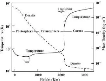
energy transfer, equation of hydrostatic equilibrium and the equation of state (including the conditions of local thermodynamic equilibrium) allows the estimation of the parameters such as absorption coeﬃcients, ionization, pressure, excitation etc (Abhyankar, 1977). The so-lar atmosphere gives a continuing challenge to soso-lar physicists and its mean parameters are presented in Fig. 2.5.

Figure 2.5 – Variation of temperature and density in the solar atmosphere (Athay, 1976).

2.3.2 The physics of Solar plasma

The magnetic field of the Sun is involved in a complex interaction with the plasma. The solar magnetic field is believed to be generated by a hydromagnetic dynamo process operating in the Sun’s interior, hence in the convective zone, due to the strongly turbulent environment, the flow-field interactions release at the Sun’s surface and then disperse into the spatial en-vironment. The turbulent electromotive force, the dynamo saturation problem, and the flux transport dynamo have been studied (Charbonneau, 2013b,a). The solar activity event occurs over the whole of the solar atmosphere by causing phenomena such as: sunspots in the pho-tosphere, the faculae near the sunspots and overlying plagues in the chromosphere, activation and eruption of the prominence and filaments in the corona. The indication of magnetic ac-tivity of the Sun is also given by its flares and the coronal mass ejection (CME) which eject the coronal matter into space. The magnetic field of the Sun is related by the solar dynamo action (Larmor, 1919; Cowling, 1933) in the convective zone, through an interaction with the differential rotation, the helical convective motions and the north-south meridional circulation (Dikpati & Gilman, 2009).

2.3.3 The outer layers of the Sun

Photosphere. The photosphere is the deepest layer of the solar atmosphere visible to the naked-eye (C. J. Durrant, 1988), where most of the Sun’s energy is radiated out. This is not a solid surface, as the Sun is totally gaseous, the rotation rate is diﬀerent for each

(25)

layer of the Sun. The flow is rising from the center of the granulation cells, cools down while it floats horizontally out toward the darker layers where it sinks down again. Features such as dark sunspots pores, sunspots (see for more Sec.3), bright faculae, granulation and super granulation are observed at the photosphere. The photosphere emits a continuous spectrum, hence it allows measurements of large flows and a pattern of waves and oscillations.

Granulation. The granulation is observed at the photosphere. This bright rounded area produces the Sun’s surface granules, and its whole structure-granulation. Typical granules have around 5 − 20 min of lifetime before dissipating (Bahng & Schwarzschild, 1961) and diameters on the order of 1500 km, after which they are divided by the appearance of new granular structures. The visible granules are explained by convective motion. The entire Sun is covered with small granulations. The granulation ﬂows can have supersonic speeds, which may produce sonic "booms", also waves at the Sun’s surface.

Super granulation. Another kind of granulation occurs below the photosphere, it is called the super granulation which is between 20000 − 40000 km in diameter with lifespans of be-tween 20 − 48 h. Several thousands of the super granulations cover the Sun’s surface. The observational data of the SOHO’s Michelson Doppler Image (MDI) helped to understand the movement and structure of plasma at the surface and deeper in the interior. Moreover analysis of the MDI’s data showed that the super granulation has a pattern of activity which is moving across the solar surface in waves (Tom Duvall, NASA).

Faculae. The solar faculae is the bright edge of the solar disk, a measurement of the visible faculae can be achieved with a spectroheliogram at the wavelengths of hydrogen or ionized calcium vapour. The appearance of faculae over the sunspots makes the Sun brighter during the sunspot cycles, being that the faculae is hotter than its surroundings, therefore looks as bright spots at the photosphere.

Chromosphere. The observable outer layers of the Sun above the photosphere constitute its chromosphere. One of the interests in the feature of the chromosphere is that temperature rises with height. A possible explanation is related to the magnetohydrodynamic waves. The chromosphere erupts as a narrow, bright red ring ambient in its corona. The chromosphere is the coldest part of the Sun’s atmosphere which allows for the existence of carbon monoxide and water as indicated in absorption spectra (Solanki et al., 1994). The chromosphere’s spectrum exhibits numerous emission and absorption lines (Abhyankar, 1977), such as helium and Ca II, helium becomes partially ionized (Hansteen et al., 1997a). The mean physical characteristics are shown in Tab.2.3.1. The chromosphere is a place of activity, hence filament eruption, flow of materials are observable over the chromosphere. Besides the ejection of materials to the corona with high speed, in the chromosphere events such as polar solar flares and prominence take place. At the outline of the chromosphere are super granules with magnetic field branches in the super granulation (Narayanan, 2012).

Transition Region. Between the cooler chromosphere and the hot corona is the irregular narrow transit region. From this region the energy emitted onto the coronal region is domi-nated by ionized carbon (IV), oxygen (V) and silicon (I) with stripped electrons (Benestad, 2002). Due to the full ionization of helium in the thin transit region the temperature increases, hence the reduction of the radiative cooling of the plasma will take place (Hansteen et al., 1997b). This highly variable zone is not easy to observe from the Earth, however it is visible from space by sensitive instruments to the extreme ultraviolet (Dwivedi, 2003). The ions emit light in the ultraviolet region of the spectrum and can be studied by TRACE and SOHO solar mission’s. The energy in the transition region is supplied from the corona as heat or as

(26)

potential energy of the elevated material which can then be radiated away or carried in the solar wind.

Corona. The corona is visible during a solar eclipse like the chromosphere, as the Sun covers up the photosphere, the white corona around the dark moon appears (Golub et al., 2010) and it is a collection of gases. The Sun’s extended atmosphere starts at its corona, with a larger volume than that of whole Sun’s photosphere. Mechanical energy dissipates while the flow moves into interplanetary space the radiation flux and the solar wind (Russell, 2001). Thus the loss of the total energy in the Sun’s corona can be carried out through the solar wind and the radiation flux. By thermal conduction and the enthalpy flow, the energy loss from the corona appears in the transition region and upper chromosphere. Due to ions with electrons from the plasma state, the corona has a high temperature. The atoms collide with sufficient energy to eject electrons, causing the ionization process to take place, in strong solar activity at temperatures from 1.3 million K to 3.6 million K (Narayanan, 2012).

Coronal mass ejection. Important events taking place in the corona is its mass ejection (CME). The CME’s have an eﬀect on the physical conditions of the interplanetary medium. The CME’s are huge clouds of ionized gas that contain 10 billion tons of material carried with the typical speed of 1000 km/s into space from the Sun, by disrupting the ﬂow of the solar wind (Vázquez & Hanslmeier, 2005). CME’s were detected as a magnetic cloud that often exhibits a three part structure, the bright active regions, the dark elongated regions in the north-south direction, which are then followed by surrounding regions. The observation of the Interplanetary Scintillation (IPS) have showed the detection of the CME on the Sun Earth environment (Manoharan et al., 1995).

Prominence. One inducer of solar activity is its prominence. The solar activity causes such activity as ﬂares and sunspots. Prominence is measurable data of Sun, which can be achieved by ground based telescopes and spacecraft such as SOHO. The solar outer layers from the solar photosphere to corona exhibit events such as coronal mass ejection, ﬂares, granulation, super granulation and faculea.

Solar wind. The source of the solar wind is the Sun’s corona which extends out into

interstellar space (Meyer-Vernet, 2007). As it pours out in to space it amounts to 10−4

M⊙

over the Sun’s age over 109

years. The spacecraft Ulysses has made a complete orbit of the Sun and mapped the speed of the solar wind, the magnetic field strength, direction and particle composition. This solar mission established that the solar wind is uniform in all directions and that the streams in the solar corona can often be used to identify the solar poles. The solar wind is not only the source of the solar mass loss, as there are other sources such as by electromagnetic waves. The interaction between Earth’s geomagnetic field and the solar wind produces storms in Earth’s magnetosphere, also seen as northern or southern lights (aurora borealis and aurora australis). The solar variability and its rotational evolution are partially linked with the magnetism. These solar magnetic field lines carry the solar wind which allows researchers to study planetary magnetospheres. These magnetic fields are frozen in the flow of the solar winds because of the high electromagnetic conductivity of the solar wind, which expends from the Sun towards space. Depending on the differential rotation of the Sun, the magnetic field links in a low latitude near to the solar equator with a slow speed and a fast wind originates in high latitudes near to the Sun’s pole.

The role of the coronal magnetic ﬁelds and the rotation of the Sun, and the sources of the solar wind is still an actual outstanding issue in solar physics which is a complex astrophysical goal.

(27)

Table 2.1 – List of some future solar missions.

Name Mission Launch date and

coun-try Instruments papers Yohkoh (sunbeam- For-merly Solar-A)

Spacecraft studied high-energy radiation from solar flares 30 August 1991,

Japan/USA/England

(Ogawara et al., 1991; Acton et al., 1992)

Ulysses Spacecraft is an international project to study the poles of the Sun and

inter-stellar space above and below the poles

6 October 1990, USA and Europe Solar Flydy

Wenzel et al. (1992)

Wind A spin stabilized spacecraft and placed in a halo orbit around the L1 Lagrange

point, more than 200 Re upstream of Earth to observe the unperturbed solar wind that is about to impact the magnetosphere of Earth.

in Novomber, 1994 US (Acuña

et al., 1995) SOHO-Solar

and Helispheric

Observatory

The main scientific purpose of SOHO is to study the Sun’s internal structure, and Sun’s corona and that gives rise to the solar wind, using imaging and spec-troscopic diagnosis of the plasma in the Sun’s outer regions coupled with in-situ measurements of the solar wind.

21 December 1995, USA Domingo

et al. (1995)

Genesis The primary objective of the Genesis mission was to collect samples of solar

wind particles and return them to Earth for detailed analysis.

8 August 2001, USA Solar Wind Sample Return

Lo et al.

(2001) ACE-Advanced

Composition Explorer

A robotic spacecraft and explorers program Solar and space exploration mission to study matter comprising energetic particles from the solar wind, the inter-planetary medium, and other sources.

25 August 1997, NASA Stone et al.

(1998) TRACE-The

objective of the

Transition

Re-gion and Coronal Explorer

The space telescopeits satellite was to explore the three-dimensional magnetic structures which emerge through the visible surface of the Sun, the photoshere and define both the geomety and dynamics of the upper solar atmosphere, the transition region and corona.

1 April 1998, NASA Handy et al.

(1999)

RHESSI-Ramaty High Energy So-lar Spectroscopic Imager

The overall objective is to explore the basic physics of particle acceleration and explosive energy release in solar flares.

5 Febrary 2002, NASA Lin et al.

(2002);

Hur-ford et al.

(2002)

Hinode

sunrise-Formerly Solar-B

Was planed to explore the magnetic fields of the sun. It consists of a coordi-nated set of optical, extreme ultraviolet, X-ray instruments to investigate the interaction between the Sun’s magnetic field and its corona

22 September 2006, Japan

Aero space Exploration

Agency Solar mission with USA and UK (Kosugi et al., 2007; Culhane et al., 2007; Golub et al., 2007; Tsuneta, 2008) 10 STEREO-Solar Terrestrial Relation Obser-vatory

Solar Terrestrial Probes program, it employs two nearly identical space based observatories-one ahead of Earth in its orbit, the other training behind-to pro-vide the first-ever stereoscopic measurement to study the Sun and the nature of its coronal mass ejections.

26 October 2006, NASA Kaiser et al.

(2008)

IRIS-Interface

Region Imaging

Spectrograph

The mission to study the crucial region by tracing the flow of energy and plasma through the chromosphere and transition region into the corona using spectrom-etry and imaging.

Operating, 27 June 2007, NASA

De Pontieu

et al. (2014)

PICARD PICARD takes simultaneous measurements of the Sun’s irraadiance, solar flares,

magnetic fields and diameter/shape, studying the link between solar cycles and temeperature changes on earth.

Operating, 15 June, 2010, CNES, France Meftah et al. (2014) SDO-Solar Dy-namics Observa-tory

SDO records the Sun’s dynamic solar activity to understand how it affects life on Earth.

2 November 2011, NASA Pesnell et al.

(2012)

SOLAR/SMO

-Solar Monitoring Observatory

SOLAR is mounted on the Columbus module of the International Space Station. It measures the irradiance received from the Sun, contributing to solar and stel-lar physics research, as well as improving atmoshperic modeling, atmospheric chemistry and climatology models.

7 February 2008, NASA Schmidtke

et al. (2006)

Solar Probe Plus Solar Probe+ will exploring what is arguably the last region of the solar system

to be visited by a spacecraft, the Sun’s outer atmosphere or corona as it extends out into space. Solar Probe+ will study the coronal heating and of the origin and evolution of the solar wind.

Development, July 2018, NASA Fox et al. (2015) DSCOVR (The Deep Space Climate Observa-tory)

The Deep Space Climate Observatory (DSCOVR) will maintain real-time solar wind monitoring capabilites critical to the accuracy and lead time of the National Oceanic and Atmospheric Administration (NOAA) s space weather alerts and forecasts. Launch vehicle on 11 February 2015, NOAA, USA Cash et al. (2012)

Aditya-1 The mission of Aditya is to study the Sun’s coronal mass ejections and magnetic

field structures. Development, 2019 − 2020, India, ISRO Sankarasubramanian (2013) Solar Orbiter-SolO

Sun-centric 25 degrees solar inclination, 0.28 AU SolO is an ESA mission to study how the Sun creates and control its heliosphere.

Lanced date is the,

Planned to be lanced in October 2018, in Florida Gandorfer et al. (2011); Woch & Gizon (2007)

Solar Sentinels Solar Sentinels contains six spacecraft (with three separated group) that will

study the sun during solar maximum of solar cycle 24, that provide to under-stand the solar storms and the deadly radiation of a solar maximum, researching energetic particles, coronal mass ejections and interplanetary shocks in the inner heliosphere.

NASSA, Planed in

2015, 2014, 2017

to be add the papers

(28)

Table 2.2 – Observational and calculated (from SSM) physical characteristics of the Sun, (Satya Narayanan, 2013). Properties Values Radius R⊙ 696.000 km Mass M⊙ 1.988 · 1030 kg Volume V⊙ 1.41 · 1027m 3 Average density ρ⊙ 1.408kg/m2 Surface gravity 273.95m/s2

Equatorial rotation 25.4 days

Polar rotation 36 days

Temperature at

sur-face T⊙

5.785 K Escape velocity at

sur-face 2.223 · 106 km/h Hydrogen abundance X 73% Helium abundance Y 25% Heavy elements Z 2% Luminosity L⊙ 3.846 · 1033erg/s

Table 2.3 – Physical properties of the solar interior (Wilson, 1994).

Zone Radius in Rsun Density [g/cm3] Temperature [K]

Core 0˘0.25(Rc) 150˘20 1.5 · 107˘7 · 106 Radioactive zone 0.25˘0.70 20˘0.2 7 · 106_{˘2 · 10}6 Tachocline Rc/R⊙ = 0.693 ∼ 0.2 ∼ 2 · 106 Convective zone 0.7˘1.0 _{∼ 0.2 · 10}−6 _{2 · 10}6_{˘7 · 10}3

Zone Extension Temperature [K] Density [g/cm3_]

Photosphere 400km 7000 − 4500 _{∼ 10}−7 Chromosphere _{∼ 10}4 km 104 ₁₀−12 Transition Re-gion ∼ 100km from 20.000 to 2 · 106 Carone R⊙ 106 ₁₀−17

Solar wins _{from 1.6 · 10}6

to 8 · 105

from 108

cm−8 _to

10cm−3 _(Schwenn,

(29)

(30)

Chapter 3 Solar activity and sunspots

We are living in the Sun’s corona.

Sydney Chapman (1957) Increased solar activity (SA) causes extreme ultraviolet and X-ray emissions from the Sun that produce effects in Earth’s upper atmosphere owing to atmospheric heating increasing the temperature and density at spacecraft altitudes. Energetic particles accelerated from the Sun, increase of solar flares and CME’s cause damage to sensitive instruments in the space environment. Photospheric and chromospheric phenomena such as sunspots, prominences, and coronal disturbances, as well as solar magnetism are all associated with solar activity. The fine structures of the sunspots are presented by many authors e.g. (Rubio, 2010). There is some evidence that variation of solar activity causes changes to Earth’s climate (Haigh, 2007), and that the variability of the Sun has had a significant impact on global climate (Bard & Frank, 2006). The origin and cause of SA is still uncertain, but there are dynamo models that predict the SA is magnetic in nature and is produced by solar dynamo processes (Charbonneau, 2005). In general two processes are used in the theory of the Sun’s dynamo models as the Ω effect-shearing and the α effect-helical motions. The structure and formation of sunspots are briefly recollected in historical sequence as outlined in Sec.2.1. In this section it was briefly summarized the general nature of solar activity and its physical characteristics, i.e. their sizes, lifetimes, brightness, evolution, Wilson depression, magnetic field and physical structure. The modern observational data are discussed in this section.

3.1 Sunspots and their general properties

The active regions of the Sun have an intense photospheric magnetic field, the magnetic flux loops into chromosphere, transition region and corona. These are manifested in differ-ent wavelengths and in differdiffer-ent layers of the Sun’s atmosphere. Dark cooler regions in the photosphere of the Sun were named "sunspots" in Galileo’s era.

General characteristics of sunspots. Sunspot groups have a high magnetic ﬁeld which has two parts, the leading sunspot in a sunspot group will have a north magnetic pole, while the trailing sunspot group will have a south magnetic pole (Thomas & Weiss, 2008; Moreno-Insertis, 1992; Minasyants & Minasyants, 2013). Sunspots move to the opposite polarity by roughly aligning east-west i.e. rotational direction of the Sun. The magnetic ﬁeld lines emerge from a spot with one polarity and re-enter another one of opposite polarity. The gaseous

(31)

CHAPTER 3. SOLAR ACTIVITY AND SUNSPOTS

Figure 3.1 – The evolution of the active regions of Sun through almost two complete solar cycles. The collage of images taken in the 284 Angstrom wavelength of extreme ultraviolet light. Abated from ESA and NASA/SOHO.

regions do not rotate with the same rate, hence at the equator the Sun rotates once every 25

days which is where the solar maximum takes place. At regions 30◦ _{above and below from the}

equator it takes 26.5 days to rotate to the start of a sunspot cycle i.e. sunspot numbers are

at a minimum on the equator. Regions at 60◦ _{from the equator take up to 30 days to rotate}

due to regions of strong magnetic ﬁeld sunspots and the switched poles will linger in total for 22 years. The small sunspot pores link with the weaker magnetic ﬁelds which are long lived in a dark region without a penumbral structure. Generally the spot pore vanishes after typical lifetimes shorter than one month, then the advance stage of pores will have acquired a penumbra forming the sunspots (Thomas & Weiss, 1992).

Sunspot cycle. Schwabe (1844) first in 1843 mentioned the periodic nature of sunspots where the records of sunspot observation varied between minima and maxima with a peri-odicity of 10 years. The maximum number of spots was as high as 250 per month but no sunspots may appear during the solar activity minimum which is know as the Schwabe cycle. The standard 11 year length of the solar cycle was established by Wolf in 1852 and that the length of the individual cycles vary between 9 and 12 years. The 11 year period of the active regions vary in rising size, number, latitude and solar activity level by reflecting magnetic field strength tracing almost similar behavior in each 11 year period. The strongest flattening of the corona takes place two years before the sunspot minima, while the weakest takes place two years before sunspot maxima. This explains that during the solar activity maximum corona is blown out in all directions and why the coronal mass ejections are observable during sunspot maximum. The Extreme Ultraviolet (EUV) and X-ray image observations show that the brighter active regions begin from the transition region which extend to the corona. The active regions of the Sun during a solar maximum and minimum are illustrated in Fig.3.1. The brighter areas in the extreme ultraviolet correspond to areas of strong magnetic fields. The strongest magnetic concentration on the Sun’s surface provides evidence of sunspots with