A 3D-CTM with detailed online PSC-microphysics: analysis of the Antarctic winter 2003 by comparison with satellite observations

HAL Id: hal-00302104

https://hal.archives-ouvertes.fr/hal-00302104

HAL is a multi-disciplinary open access

archive for the deposit and dissemination of sci-entific research documents, whether they are pub-lished or not. The documents may come from teaching and research institutions in France or abroad, or from public or private research centers.

L’archive ouverte pluridisciplinaire HAL, est destinée au dépôt et à la diffusion de documents scientifiques de niveau recherche, publiés ou non, émanant des établissements d’enseignement et de recherche français ou étrangers, des laboratoires publics ou privés.

A 3D-CTM with detailed online PSC-microphysics:

analysis of the Antarctic winter 2003 by comparison

with satellite observations

F. Daerden, N. Larsen, S. Chabrillat, Q. Errera, S. Bonjean, D. Fonteyn, K.

Hoppel, M. Fromm

To cite this version:

F. Daerden, N. Larsen, S. Chabrillat, Q. Errera, S. Bonjean, et al.. A 3D-CTM with detailed online PSC-microphysics: analysis of the Antarctic winter 2003 by comparison with satellite observations. Atmospheric Chemistry and Physics Discussions, European Geosciences Union, 2006, 6 (5), pp.8511-8552. �hal-00302104�

ACPD

Printer-friendly Version Interactive Discussion Atmos. Chem. Phys. Discuss., 6, 8511–8552, 2006

www.atmos-chem-phys-discuss.net/6/8511/2006/ © Author(s) 2006. This work is licensed

under a Creative Commons License.

Atmospheric Chemistry and Physics Discussions

A 3D-CTM with detailed online

PSC-microphysics: analysis of the

Antarctic winter 2003 by comparison with

satellite observations

F. Daerden1, N. Larsen2, S. Chabrillat1, Q. Errera1, S. Bonjean1, D. Fonteyn3, K. Hoppel4, and M. Fromm4

1

Belgian Institute for Space Aeronomy BIRA-IASB, Brussels, Belgium

2

Danish Meteorological Institute, Copenhagen, Denmark

3

Belgian Federal Science Policy, Brussels, Belgium

4

Naval Research Laboratory, Washington D.C., USA

Received: 13 June – Accepted: 17 August 2006 – Published: 12 September 2006 Correspondence to: F. Daerden (Frank.Daerden@aeronomie.be)

ACPD

Printer-friendly Version Interactive Discussion

Abstract

We present the first detailed microphysical simulations which are performed online within the framework of a global 3-D chemical transport model (CTM) with full chem-istry. The model describes the formation and evolution of four types of polar strato-spheric cloud (PSC) particles. Aerosol freezing and other relevant microphysical

pro-5

cesses are treated in a full explicit way. Each particle type is described by a binned size distribution for the number density and chemical composition. This set-up allows for an accurate treatment of sedimentation and for detailed calculation of surface area densities and optical properties. Simulations are presented for the Antarctic winter of 2003 and comparisons are made to a diverse set of satellite observations (optical and

10

chemical measurements of POAM III and MIPAS) to illustrate the capabilities of the model. This study shows that a combined resolution approach where microphysical processes are simulated in coarse-grained conditions gives good results for PSC for-mation and its large-scale effect on the chemical environment through processes such as denitrification, dehydration and ozone loss. It is also shown that the influence of

15

microphysical parameters can be measured directly from these processes.

1 Introduction

Polar stratospheric clouds (PSCs) play a double key role in springtime polar ozone depletion, see e.g.Solomon (1999); WMO(1999); Dessler (2000); Tolbert and Toon (2001) and references therein. The surface of the PSC particles serves as a catalizing

20

substrate for heterogenous reactions which transfer chlorine from reservoir species to active species. Upon photolysis these active species release atomic chlorine which in its turn ignites catalytic ozone destruction cycles. The process of chlorine activation would be severely underestimated without taking into account the catalyzing role of PSCs.

25

The second key role of PSCs in ozone depletion is indirect in the way that they control 8512

ACPD

Printer-friendly Version Interactive Discussion the nitrogen budget of the polar stratosphere, at first temporarily through the uptake

of nitric acid, a process called denoxification. Then when the particles grow large enough to reach substantial fall velocities, they will sediment and permanently remove the absorbed nitrogen from the stratosphere, this process is called denitrification. Such a situation in which the polar stratosphere becomes permanently depleted from nitrigen

5

throughout the polar winter and spring will delay the deactivation of active chlorine back into the reservoir species and as a consequence prolong the ozone depletion conditions.

As liquid PSC particles (Supercooled Ternary Solutions, STS) are not expected to grow very large the current general view is that only solid particles can cause

denitrifi-10

cation. Besides ice particles, which freeze out of STS at very low temperatures, nitric acid trihydrate (NAT) has progessively been regarded as a second important type of solid PSC particle (Voigt et al.,2000;Fahey et al.,2001). Not only is NAT a remnant of evaporation of ice particles, but recent research indicates that NAT can also form out of metastable nitric acid dihydrate (NAD) which may freeze out of STS at temperatures

15

above the ice frost point (Tabazadeh et al.,2002). This means that NAT may nucleate and grow at higher temperatures than ice.

In the past various models have been developed to understand how PSCs form and evolve and to study their influence on the chemical environment. Most of these models are defined as Lagrangian box models, e.g. the DMI microphysical model used in the

20

present study (Larsen,2000) has been extensively used for studies of PSC evolution on trajectories (Larsen et al.,2002,2004;Svendsen et al.,2002;H ¨opfner et al.,2006a). The IMPACT model (Drdla,1996;Drdla et al.,2003) couples a detailed microphysical description and a full chemistry approach on trajectories. Various models estimate the effect of PSCs on the chemical fields by using a simplified growth and sedimentation

25

scheme. The CLaMS model (Grooß et al., 2002;Konopka et al.,2004) follows such an approach combined with a full chemical description on trajectories. A difficulty with trajectory models concerns the handling of sedimentation. In the mentioned models various approaches have been used to deal with this problem. The most common

ACPD

Printer-friendly Version Interactive Discussion solution consists in determining the fall velocity of the largest particles and deriving

from this a downward flux for H₂O and HNO₃, eventually combined with a parametriza-tion for particle evaporaparametriza-tion (Grooß et al., 2004). The IMPACT model uses a more complex approach based on the flexible grid concept of M ¨uller and Peter (1992). A different approach aimed specifically at the study of denitrification is used in Carslaw

5

et al. (2002). In this study a denitrification scheme (DLAPSE) is defined on trajectories in which the sedimentation of particles is treated analytically. This scheme is coupled to the SLIMCAT 3-D chemical transport model (CTM) (Chipperfield,1999). This ap-proach has been succesful in determining the magnitude and spatial distribution of denitrification in several Arctic winters (Mann et al.,2003;Davies et al.,2005). More

10

simplified efforts to study the effect of PSCs on chlorine and hence ozone chemistry are used by many 3D-CTMs which incorporate PSC parametrizations based on the ther-modynamical conditions. Such approaches seem to be sufficient for what concerns the large-scale effect of PSCs on the chemistry. A problem is that important processes such as denitrification have to be parametrized in some way in such models.

15

The model presented in this paper is, to the best of our knowledge, the first Eulerian 3D-CTM to incorporate detailed PSC microphysics, including an explicit treatment of sedimentation. It is a more generalized continuation of the work ofFonteyn and Larsen (1996) which studied PSC formation in a 2-D context. The microphysical model we use studies ensembles of particles in detail by following their evolution through a fixed

20

binned size distribution in which the number densities and the chemical composition of all particle types are stored. This detailed microscopical information allows for the explicit calculation of various quantities both microscopic (e.g. surface area densities) and macroscopic (such as optical properties of clouds, e.g. extinction). The binned ensemble of particles is treated as a full part of the CTM and is advected in a similar

25

way as the chemical gas-phase species. The bin structure also allows for an explicit description of sedimentation. Indeed, for each size bin the fall velocity can be calcu-lated and hence the number of particles falling out of that bin over one model time step. Because fixed size bins are used in the model, the sedimenting particles can take their

ACPD

Printer-friendly Version Interactive Discussion appropriate place in the size bins at the lower vertical model level.

All this makes it possible to compare the model output to various simultaneous ob-servational datasets as diverse as optical properties and chemical concentrations. Be-cause the model treats ice as well as NAT particles in a general way, it is applicable to both Arctic and Antarctic winters. In this paper we will present results for the Antarctic

5

winter of 2003, and compare them to observations of MIPAS/Envisat (tracer evolution, denitrification, dehydration and ozone depletion) and POAM III (aerosol and PSC ex-tinction, dehydration, ozone depletion). Results for Arctic winters will be presented in future publications.

Section2resumes the key facts of the PSC and CTM models. In Sect.3the results

10

for the Antarctic winter 2003 will be presented, followed by a summary in Sect.4.

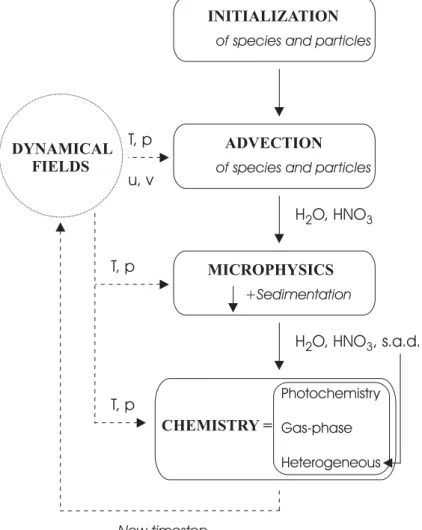
2 The PSC and CTM models

The coupled PSC-CTM model is developed at BIRA-IASB. This model is the core model of the fourdimensional variational (4D-VAR) chemical data assimilation system BASCOE, the Belgian Assimilation System of Chemical Observations from Envisat

15

(Errera and Fonteyn,2001;Fonteyn et al.,2002,2004). The PSC part is described in Larsen(2000). Here we will briefly summarize the main characteristics of the model. 2.1 The 3D-CTM

This 3D-CTM integrates in time the volume mixing ratios of 57 gas-phase species relevant for stratospheric chemistry. The horizontal resolution is variable and for the

20

present study two resolutions have been used:

– low resolution: 3.75◦in latitude and 5◦ in longitude (with∆t=30 min.)

– high resolution: 1.875◦ in latitude and 2.5◦in longitude (with∆t=15 min.) 8515

ACPD

Printer-friendly Version Interactive Discussion This means that for the higher resolution the latitudinal size of a model grid cell is

about 200 km and the longitudinal size ranges in the polar region from 140 km at 60◦to e.g. 25 km at 85◦. (We will comment later in this paper on the influence of model res-olution.) The model is defined on 37 vertical levels, of which the 28 upper levels are identical to the ECMWF stratospheric pressure levels and the remaining 9 levels are a

5

subset of the ECMWF hybrid tropospheric levels (in the 60-level product). The model’s vertical range is from 0.1 hPa down to the surface. The advection scheme is the flux form semi-Lagrangian transport algorithm ofLin and Rood(1996). The model is driven by the 12 to 36 h ECMWF operational forecasts, which are interpolated to a 1◦×1◦grid before downloading, and finally averaged in a mass-conservative way to the relevant

10

CTM grid. The choice for using forecast fields was inspired byMeijer et al.(2004) in which forecast fields are shown to be less diffusive than 4D-VAR analyses. Since we intend to do runs of about 6 months, we opted for the forecasts. The model integra-tion timestep is 30 min in the low resoluintegra-tion and 15 min in the high resoluintegra-tion case. The chemistry module is built by the Kinetic PreProcessor (Damian et al., 2002) and

15

is integrated using a third-order Rosenbrock solver (Hairer and Wanner, 1996). The 57 chemical species interact through 143 gas-phase reactions, 48 photolysis reactions and 9 heterogeneous reactions, all listed in the latest Jet Propulsion Laboratory com-pilation (Sander et al.,2003). It is important to note that the chemistry module includes the heterogeneous reactions and that photochemical, gas-phase and heterogeneous

20

reactions are solved as one chemical system, in which the surface area densities are provided by the microphysical module.

2.2 The PSC module

The PSC module of DMI (Larsen, 2000) is interactively coupled to the 3D-CTM. It describes the evolution in size distribution of the number density and chemical

compo-25

sition of 4 types of particles, listed in Table1. The size distribution of all particle types is binned on a geometrically increasing volume scale. For the present study the range in particle radius of the bins is 0.002–36 µm and the number of bins is 36. In each

ACPD

Printer-friendly Version Interactive Discussion bin 4 quantities are stored: the particle number density and the masses per particle

of respectively condensed sulfuric acid, nitric acid and water. Besides the ambient air temperature and pressure, the PSC module is called with the model partial pressures of water vapor and nitric acid as inputs. These model fields can be changed by the PSC module, as the particles may take up or release water or nitric acid as a consequence

5

of their microphysical evolution. The combined surface area density of all particles on a model gridpoint is used to calculate the heterogeneous reaction rates which are served as an input to the chemistry module. This illustrates the interactive nature of the coupling between the 3D-CTM and the PSC module, which is schematically presented in Fig.1. The PSC module has an internal timestep because the microphysical

pro-10

cesses may require computational timescales much smaller than the CTM timestep. This internal timestep is made variable to gain computing time and is determined by the smallest timescale involved in the microphysical processes relevant in a specific call to the module.

The microphysical processes described by the module are, schematically (see

15

Larsen(2000) for a detailed discussion):

1. homogeneous volume dependent nucleation of ICE out of STS 3–4 K below the ice frost point temperature T_ice (Koop et al., 2000), and homogeneous surface dependent nucleation of nitric acid dihydrate (NAD) out of STS (Tabazadeh et al., 2002) above T_ice, followed by (assumed) instantaneous conversion of NAD to

20

NAT.

2. nucleation of NAT by vapor deposition of HNO₃ and H₂O on pre-activated SAT (Zhang et al.,1996), and nucleation of ICE by vapor deposition of H₂O on NAT; 3. dissolution of SAT into STS at low temperatures in the presence of high HNO₃

concentrations in the gas phase, followed by uptake of H₂O and HNO₃ (Koop

25

and Carslaw, 1996), and melting of SAT into liquid sulfate aerosols particles at temperatures above 216 K;

ACPD

Printer-friendly Version Interactive Discussion 4. condensation and evaporation of HNO₃and H₂O to and from STS, NAT and ICE,

using the basic vapor diffusion equation and applying a full kinetic approach; 5. mass balance calculations of HNO₃and H₂O between gas and condensed phase; 6. sedimentation of particles (Pruppacher and Klett, 1997; Fuchs, 1964). As the size bins are the same everywhere in the model, particles sedimenting from one

5

model layer to the lower one can fall into the appropriate size bin.

Recent studies seem to indicate that the homogeneous freezing rates for NAD have to be reduced considerably (Larsen et al.,2004;Irie et al.,2004). We will investigate the effect of reducing the theoretical homogeneous freezing rates by 100.

To compare with extinction measurements the extinction of the aerosols and PSCs

10

are calculated in the model. This is done using by Mie scattering theory for the spher-ical particles (STS) and the T-matrix technique (Mishchenko and Travis,1998) for the nonspherical particles (SAT, NAT, ICE). For the T-matrix calculations a database of ex-pansions of the elements of the scattering matrix in generalised spherical functions is used. The recommendations of Mishchenko and Travis(1998) for input parameter

15

settings have been followed. The database used is for volume-equivalent sizes and an imaginary refractive index of 10−8. The real refractive indices used are taken from Krieger et al. (2000) and Scarchilli et al. (2005). For the nonspherical particles an aspect ratio of 1.05 is assumed.

3 Antarctic winter 2003

20

In this section we present results of simulations for the Antarctic winter of 2003 and comparisons to satellite observations.

ACPD

Printer-friendly Version Interactive Discussion 3.1 Observational datasets and methodology

For this study of the Antarctic winter 2003 we will compare model results to observa-tions from MIPAS/Envisat and POAM III. Here we will shortly present the instruments and their datasets, and the methodology followed for the comparisons.

MIPAS, or the Michelson Interferometer for Passive Atmospheric Sounding, is a

limb-5

scanning Fourier transform infrared spectrophotometer (Fischer and Oelhaf, 1996; ESA,2000) onboard Envisat. Envisat’s orbit time is 101 min resulting in about 14 orbits per day. There are usually around 1000 MIPAS profiles available per observed species per day. Each profile has at most 17 points ranging from about 6 km to about 60 km. The chemical species observed by MIPAS are O₃, HNO₃, H₂O, NO₂, N₂O and CH₄.

10

We use the offline reprocessed data version 4.61 for our comparisons.

POAM III is a visible/near infrared solar occultation photometer onboard the French Spot-4 satellite which measures the chemical stratospheric constituents O₃, H₂O and NO₂, and aerosol extinction in the polar regions (Lucke et al., 1999; Lumpe et al., 2002). Here we use the POAM III version 4 data. Throughout this text we will denote

15

POAM III by POAM. POAM profiles have a vertical resolution of 1 km. The aerosol extinction profiles reach up to 25 km. The chemical species profiles have a wider al-titude range. The POAM line of sight is about 230 km. POAM measures at most 15 profiles per day in each hemisphere, all these profiles are located at a fixed latitude and with a longitude spacing of about 25◦. The latitude at which the profiles are taken

20

varies slowly throughout the year, but remains in the polar region. In Antartic winter periods, the latitude varies smoothly between about 65◦S (winter solstice) and about 87◦S (equinox).

To provide a uniform set-up for the comparison of model results to measured profiles the following methodology will be applied. The model data have been interpolated in

25

space and time (co-located) to the observed profiles. This interpolation occurs online, i.e. at the model timestep where a profile is available. This way of working guarantees an optimal comparison, e.g. in the case of rapidly changing PSC fields. In a practical

ACPD

Printer-friendly Version Interactive Discussion sense it allows for a considerable limitation in model output and hence disk space

us-age. Then the observed and co-located model profiles, as well as the observational errors, are interpolated to 4 isentropic levels: 425 K, 475 K, 525 K and 575 K (corre-sponding to pressure values of approximately 70 hPa, 50 hPa, 30 hPa and 20 hPa and to altitudes of approximately 17.5 km, 20 km, 22.5 km and 25 km inside the vortex). Of

5

the interpolated data at these levels the error-weighted average is calculated over 5-day intervals. Since we concentrate on polar winter processes only profiles within the polar vortex are taken into account, with the vortex edge being calculated following the definition ofNash et al. (1996) using the dynamical fields interpolated to the high-resolution model grid (see Sect.2.1). Although we will call the quantities obtained in

10

this way error-weighted mean vortex values, it is important to note that they can not be regarded as properly vortex-averaged values, but merely as averages of available values within the vortex.

When POAM samples a water ice cloud, the large solar extinction prevents POAM from performing a measurement. Such points have been removed in the corresponding

15

model data as well before taking the average. Also observations with a negative error have been removed in both the observed and model profiles before taking the average. Negative data, e.g. some POAM extinction measurements, have not been removed because they are meaningful observations as long as their absolute value is smaller than the retrieval random error.

20

We have chosen to present 5-day averages because they result in much clearer plots than e.g. daily averages. For example, variability in the POAM extinction data is a convolution of the zonal asymmetry of PSC occurence and composition, seasonal evolution of PSC forcing, and POAM sampling. Here we list a number of issues which could lead to a difference in variability between the model and the observations. POAM

25

has a long line of sight in which various PSC particles could be sampled at various dis-tances (within the same atmospheric layer) rather than that they would all be located at the tangent point, which is where the model calculations are done. Furthermore the model produces clouds which are limited by the model’s grid size in coarse-grained

ACPD

Printer-friendly Version Interactive Discussion conditions and which have uniform properties inside a grid cell. But as an occultation

instrument, and even though its retrieval region is comparable to the model’s horizontal grid size, POAM could well sample small localized clouds of high extinction. These will then spureously be considered as being uniformly distributed over the effective absorp-tion region near the tangent point, leading to an increased extincabsorp-tion value which will

5

be underestimated by the coarse-grained model. Also as an occultation instrument, POAM has a much higher vertical resolution than the model. And finally it is obvious that the coarse-graining of the temperature to the model resolution will have some influ-ence. The aim of the present study is however not to analyze and eventually correct for this detailed variability (e.g. by introducing sub-grid scale mountain wave

parametriza-10

tions) but rather to test the overall performance in polar winter processes of the PSC model in the coarse grained model conditions. For this 5-day averages are sufficient.

In the following we will show comparisons of model data for all observed fields ex-cept for NO₂, which is nearly completely transformed into HNO₃ under polar winter conditions (Kawa et al.,1992), and CH₄, which has a behavior comparable to N₂O.

15

3.2 Initializations

The simulations start on 1 May 2003 and run until 15 December 2003. The model’s chemical fields are initialized from an assimilation of MIPAS/Envisat observations with the 4D-VAR chemical data assimilation system BASCOE (Errera and Fonteyn,2001; Fonteyn et al.,2002,2004). An exception has been made for polar water vapor. It has

20

been observed that there is a substantial systematic difference in polar water vapor as observed by MIPAS and by POAM, with MIPAS water lower by up to about 25% as compared to POAM in the lower stratosphere. When the model is initialized by the MIPAS water vapor in the polar regions, it underestimates the PSC extinction as measured by POAM (not shown). This is much less the case when the model’s initial

25

water vapor field is scaled in the polar regions to match the POAM measurements. Therefore we have chosen for the latter option. MIPAS v4.61 H₂O data are validated so far only outside of the polarhoods (Oelhaf et al., 2004). In the recent validation

ACPD

Printer-friendly Version Interactive Discussion study by Lumpe et al. (2006) it is found that POAM sunset measurements of water

vapor show a systematic high bias of about 25% in the lower Antarctic stratosphere relative to HALOE, while the bias is considerably lower for the sunrise measurements. HALOE is suggested to have a 5% low bias (Harries et al.,1996;Kley et al.,2000). The latter study also shows that HALOE can show low biases of up to 15–20% with in-situ

5

measurements. Because the differences between POAM and MIPAS are comparable to the POAM-HALOE bias, and given the suggested biases in the HALOE data, we assume that tuning the model’s initial state to POAM water vapor is justifiable for the purposes of this paper. The scaling of the initial (assimilated MIPAS) water vapor field is done by deriving scaling factors from a 10-day mean POAM water vapor profile in

10

early May 2003 and the corresponding mean model profile. Then these scaling factors are applied to the initial model state everywhere poleward of 60◦ latitude.

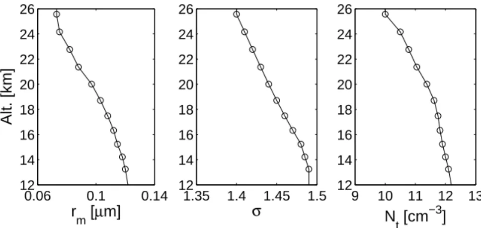
The initial sulfate aerosol size distributions are described by a lognormal function, defined by a median radius r_m, geometrical standard deviation σ and number density

N_t(Pinnick et al.,1976). We estimated these parameters on the condition that the initial

15

lognormal distribution should reproduce the Unified POAM reference background 1µm extinction monthly means (Fromm et al.,2003). This condition leaves a lot of arbitrari-ness in fixing the lognormal parameters. We have chosen to take a set of parameters that follow a smooth profile and deviate not too far from the measurements made by the University of Wyoming’s optical particle counter (Deshler et al.,2003) on balloon

20

flights in the Antarctic over the past decade (T. Deshler, private communication). Our estimated parameters are shown in Fig.2. We will comment later in this paper on the influence of the choice of these parameters.

In the following we will study model runs with four different set-ups which will be denoted by:

25

– LR : low resolution

– LR100 : low resolution with NAD freezing rates reduced by a factor 100 (see

Sect.2.2)

ACPD

Printer-friendly Version Interactive Discussion

– HR : high resolution

– HR100 : high resolution with NAD freezing rates reduced by a factor 100

In the HR simulation the background aerosol distribution is updated each month except for gridpoints with temperatures below 220 K, where the microphysics is likely to play a role. In the other simulations this methodology has not been followed, and the

5

evolution of the initial background aerosol distribution is followed throughout the winter and springtime.

3.3 Chemical tracers

In order to check how well the model calculates the atmospheric transport, and more specifically the adiabatic descent of air in the vortex and the dynamical isolation of the

10

vortex, we have compared the evolution of inactive tracer species in the vortex with observational data. A badly performing transport would have significant influence on the chemical evolution. Here we compare to the temporal evolution of N₂O as observed by MIPAS following the methodology described in Sect.3.1. The results are shown in Fig.3.

15

The simulations indicate that the numerical diffusion between the N₂O depleted vor-tex and the surrounding areas is very large and disturbs the isolation of the vorvor-tex considerably. This numerical effect is resolution-dependent and is present in all chemi-cal and particle fields with a large gradient over the vortex edge (e.g. O₃, PSCs). When the resolution is too low model grid cells located over the vortex edge sample regions of

20

air both inside and outside the vortex and replace them by a single average value. This increases the values in the region where they are the lowest and vice versa (e.g. for N₂O: increase inside the vortex and decrease outside). The effect decreases with in-creasing resolution. In our high resolution simulations the vortex mean N₂O remains acceptable close to the observations – i.e. well within the MIPAS variability – until the

25

second half of September. By this time most of the polar winter processes are over and the vortex starts to weaken. After this period the model basically overestimates

ACPD

Printer-friendly Version Interactive Discussion the mixing of polar air when the vortex disappears. It is expected that this could be

solved by using a still higher resolution but such a study was beyond the limits of the present computing power.

Results for CH₄ which is also measured by MIPAS are similar but the effect of nu-merical diffusion is smaller (not shown).

5

3.4 Extinction

Figure4shows the comparison of the calculated extinction at 1020 nm to the extinction as measured by POAM following the methodology described in Sect.3.1. The agree-ment between model and observations is good. The correspondence is excellent on the lowest two levels. The model follows the general trend of the observations with the

10

onset of enhanced extinction in June, the maximum in July and August, and the end of enhanced extinction in September 2003. A general discussion of the differences in variability between POAM and the model was already held in Sect.3.1. As already mentioned there 5-day averages remove much of the small time-scale and inter-profile variability, and here they indicate that the model produces an acceptable average

ex-15

tinction.

On the higher levels the model predicts the onset of enhanced extinction by mid-May which is two to three weeks too early compared with the observations. It is unclear wether this problem in the early winter is due to the biases in the ECMWF temper-atures or reflects a problem in the model. Gobiet et al. (2005) and H ¨opfner et al.

20

(2006b) have reported considerable temperature biases in ECMWF analyses in this period (up to 3.5 K). The forecast fields which we use are initialized by these analyses and it is likely that these temperature biases propagate in the forecast fields. Reducing the NAD homogeneous freezing rates by 100 clearly improves the situation in early winter, but on the other hand leads to an underestimation of the extinction in August.

25

When comparing 5-day median values the deviations in early winter between model and observations are even more pronounced (not shown).

The difference between HR and the other simulations in springtime is due to the 8524

ACPD

Printer-friendly Version Interactive Discussion mentioned monthly reloading of the background aerosol distribution (Sect.3.2). The

model runs with no reloading do not reproduce the actual background aerosol distri-bution, because there is no mechanism in the model to reload aerosols to the upper stratosphere to replace the aerosols which have been removed by PSC formation and sedimentation. This shortcoming is only playing a role at the 575 K level.

5

In Fig.5a we plotted the contribution of the various particle types to the total model extinction of simulation HR100. This plot illustrates that in the model the main NAT for-mation period occurs in the early winter (throughout June) while STS is the major PSC type after that period, interspersed with some intermittent ICE activity, which only rarely exceeds the STS extinction. However we remind that POAM is prevented from making

10

measurements of optically thick water ice clouds, and that the corresponding points in the co-located model profiles have been removed in the comparison, so Fig.5a does not give an indication of the actual ICE presence. Also shown is the model’s back-ground aerosol extinction, which is initialized in May from the Unified POAM reference background. This clearly illustrates the enhancement of extinction during the

winter-15

time due to PSC formation.

To analyze the early-winter situation a little further we have zoomed in on this period and plotted only the contributions of STS and NAT to the total model extinction in Fig.5b for both high resolution simulations. Clearly, reducing the freezing rates decreases the NAT contribution and increases the STS contribution, as fewer NAD particles are

nu-20

cleated from STS per timestep. Except at the lowest level the NAT extinction exceeds the STS contribution everywhere from mid-May onwards in the simulations with unre-duced freezing rates. When the homogeneous NAD freezing rates are reunre-duced by a factor 100 the temporal evolution of the NAT extinction corresponds very well with the evolution of the total POAM extinction. Indeed a strong enhancement in NAT

extinc-25

tion after the first week of June on the highest levels occurs almost simultaneously with the sudden enhancement in the POAM extinction. In the weeks before before this enhancement the overestimated extinction in the case with reduced freezing rates is caused by STS only. The STS growth and hence its extinction are controlled by

ACPD

Printer-friendly Version Interactive Discussion temperature and the gasphase H₂O and HNO₃ concentrations. It has been verified

that initializing the simulations with the MIPAS assimilated H₂O rather than the POAM-tuned H₂O does not solve the problem completely (not shown), giving indication that temperature biases may be responsible for the problem. Simulations with an overall temperature increment of 2 K improve the situation considerably (not shown).

5

Now we will study the influence of the calculated PSCs on the chemical fields in the vortex.

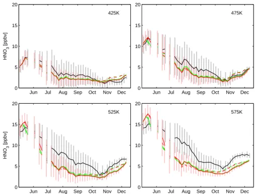
3.5 Denitrification

Figure6 shows the comparison of HNO₃ between the model and MIPAS. The model overestimates the removal of nitric acid everywhere, but this overestimation is much

10

larger on the highest two levels, while on the lowest two levels the correspondence be-tween model and the observations is acceptable (i.e. they remain within each other’s variability). The main difference between the simulations and the observations con-cerns the onset and rate of HNO₃ removal. As shown inTabazadeh et al.(2000) the early winter is the period when extensive denitrification occurs. The overestimation of

15

HNO₃removal in the early winter period is likely to be a consequence of the too early onset and overestimation of enhanced PSC presence in this period, see Fig.4. Unfor-tunately there are some data gaps in June exactly during the start of the denitrification process, but from the data which are available we notice an influence of the freezing rate reduction. The reduced freezing rates lead to a small delay in the onset of

deni-20

trification and seem to be closer to the observed values (although the data gap at the end of May makes it difficult to make precise conclusions). This would be consistent with the small delay in onset of enhanced PSC extinction of Fig.4 in the same pe-riod. As a consequence the freezing rates reduction results in HNO₃values which are slightly closer to the observations during mid-June, when there are again some data

25

available. Nevertheless the rate of denitrification in mid-June is overestimated in all simulations, which is consistent with the overestimation of the extinction in this period. By the second half of July the rate of HNO₃ removal in model and observations

ACPD

Printer-friendly Version Interactive Discussion comes comparable, but because the model has removed too much HNO₃ before this

date, its HNO₃values are much lower than the observed levels.

As already mentioned in Sect. 3.4 the possible influences of cold temperature bi-ases could be responsible for this problem. The removal of HNO₃is a combination of denoxification and denitrification. Denoxification is quite sensitive to temperature

bi-5

ases, and an overestimated denoxification will lead to an overestimated denitrification. In the following we will try to study the process of denitrification both qualitatively and quantitatively.

As shown in e.g.Popp et al.(2001) there is a narrow correlation between the chem-ical tracer species N₂O and the total amount of reactive nitrogen NO_ybefore the start

10

of the polar winter. In a denoxified and denitrified situation the total NO_y will deviate from this correlation with N₂O. This makes this correlation a useful tool to check the influence of PSCs on the nitrogen budget of the stratosphere. The only NO_y species measured in the standard MIPAS product are HNO₃ and NO₂, but the latter is rapidly converted into HNO₃ during the polar night. In fact as was demonstrated in Kawa

15

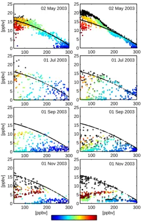
et al. (1992) in polar winter conditions NO_yconsists almost entirely of HNO₃, so for the observations of MIPAS we can approximate the NO_y–N₂O correlation by a correlation between HNO₃and N₂O. In Fig.7we show scatterplots of HNO₃versus N₂O of MIPAS and co-located HR100 model data for four different days: 2 May, 1 July, 1 September and 1 November. The plot of 2 May illustrates that the relation of Popp et al.(2001),

20

which was obtained for the Arctic winter of 1999–2000, is sufficiently valid for the 2003 Antarctic winter. Only above ∼550 K the deviations between HNO₃ and NO_y are vis-ible in the model data. The effect of ongoing denitrification is clear in the plots for 1 July, and a state of nearly total denitrification is visible in the plots for 1 September. By November 1 mixing of extra-vortex air with a higher potential temperature is occuring,

25

and also the repartitioning of nitrogen within the NO_yfamily is illustrated in the figure. The amount of denitrification can be calculated as the difference between NO_yunder polar winter and early springtime conditions and the estimated pre-winter NO_y concen-tration given by the correlation with N₂O. An approximative value for denitrification as

ACPD

Printer-friendly Version Interactive Discussion observed by MIPAS can then be calculated as the difference between the observed

HNO₃and NO_y as derived from the observed N₂O (Davies et al.,2005). We use this approximative denitrification quantity to compare the model to the MIPAS data, see Fig.8. The modeled denitrification remains very close to the MIPAS result on the low-est levels. On the highlow-est levels the onset of the denitrification in the model starts

5

too early and the initial rate of denitrification is overestimated, leading to a propagated overestimation throughout the winter. As in the comparison of HNO₃(Fig.6) the simu-lations using reduced NAD freezing rates slightly delay the denitrification onset, leading to denitrification values which are closer to the observed ones in mid-June.

The deviations during late-winter and early springtime originate mainly from the

prob-10

lem with N₂O (see Fig.3) due to numerical diffusion. 3.6 Dehydration

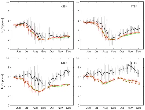
Figures9and10show the evolution of water vapor as observed by respectively MIPAS and POAM and the corresponding model results. The differences in polar water vapor data from both instruments which were already mentioned in Sect. 3.2 are obvious

15

from these plots.

Dehydration occurs because water-rich ice particles sediment when they have grown sufficiently large. The MIPAS data (Fig.9) show very little variation in the polar vortex water field throughout the winter. The POAM data of Fig.10 show much more vari-ability and the effect of dehydration is clearly visible. Dehydration starts slowly in June

20

2003, some weeks later than denitrification which is consistent with earlier studies, e.g. Tabazadeh et al. (2000). Then it continues increasingly rapidly throughout July until the beginning of August, when the polar stratospheric water vapor reaches a min-imum. At this point about 60% of the initial water vapor amount has been removed. From then on the water vapor starts to increase again very slowly with the rise of

tem-25

peratures, the evaporation of PSCs, the weakening of the vortex and the mixing with extra-vortex air. Substantial dehydration is only present below ∼525 K. All these results are consistent with a recent study of dehydration during the 1998 Antarctic winter using

ACPD

Printer-friendly Version Interactive Discussion the IMPACT trajectory model (Benson et al.,2006).

At the 525 K level the model predicts some dehydration but this is not consistent with the observations. This level is the location of a strong vertical gradient in the water vapor field. The deviations between the model and the POAM observations may well be a consequence of the coarse vertical model resolution, which may lead to an

5

overestimated smoothing of the water vapor gradient at this level.

Finally it is obvious that the deviations in water vapor, especially during mid-winter, are partly responsible for the underestimation in the model extinction during this period (Fig.4).

3.7 Ozone depletion

10

Finally we have compared the evolution of model polar ozone to observations of MIPAS and POAM. The results are shown in Figs. 11 and12. The model simulations for all set-ups reproduce the observations very well during the winter. When in the springtime the polar vortex becomes depleted with ozone due to chemical destruction, and the surrounding area, in full sunlight and in absence of active chlorine, becomes enhanced

15

with ozone, the numerical diffusion will play an important role. During the maximum of the ozone hole conditions (second half of September and throughout October) the low resolution simulations stay about 0.5–1 ppmv above the observations. The high resolution simulations improve these deviations by ∼50% at the lowest levels, while they nearly match the MIPAS data at the higher levels.

20

It is obvious from the plots that horizontal resolution is the main key to accurately simulating the ozone depletion of the vortex. This indicates that the PSC modelling and the related chemical processes are performing well. Good agreement is most difficult to reach at the lowest levels because the observed ozone concentrations on those levels are nearly zero, making the simulations very sensitive to numerical diffusion.

25

It concerns here not only a problem due to the numerical diffusion of ozone alone across the vortex edge but an accumulated effect of the numerical diffusion in various fields with strong cross-vortex edge gradients such as HNO₃(Fig.6, and the resulting

ACPD

Printer-friendly Version Interactive Discussion denitrification, Fig.8), the PSCs, and active chlorine.

Our conclusion is consistent with the study of Hoppel et al. (2005), which demon-strated that accurate dynamics is a key ingredient for correctly modeling the spatial distribution of Antarctic ozone loss.

3.8 Model sensitivities

5

Figures 11 and 12 illustrate that the effect on ozone depletion of numerical mixing due to horizontal resolution limitations is much larger than the microphysical effect of different NAD homogeneous freezing rates which have been studied here. The main influence of the NAD homogeneous freezing rates seems to be situated in the early winter and more specifically in the onset and rate of denitrification. Higher freezing

10

rates imply that more NAD (and NAT) particles are formed in the same time interval so the available nitric acid will be taken up faster than in the case with lower freezing rates, where less particles will be nucleated. When in early winter the temperatures become low enough for NAD nucleation, the simulations with higher NAD freezing rates will generate more NAT particles and the denitrification will start sooner and take place

15

faster in those simulations. When the state of nearly total denitrification is reached in July the results seem not to depend much on the NAD freezing rates anymore.

The influence of the choice of Fig. 2 of parameters for the lognormal background aerosol distribution has also been studied to some extent. The main conclusion of this study is that when the initial total number density of aerosols is too small, these

20

few particles grow too large in size since they have all nitric acid at their disposal. The sedimentation occurs too fast and the polar stratosphere becomes nearly depleted with aerosols by mid-winter. Then from mid-winter onwards the PSC extinction is severely underestimated and as a consequence the model fails to reproduce the springtime ozone depletion.

25

Finally we also studied the influence of the number of size bins used to describe the the aerosol and PSC distributions. Also here we only mention the main conclusions of this test. We have increased the number of bins up to 96, but no significant

ACPD

Printer-friendly Version Interactive Discussion ments have been found, indicating that 36 size bins is a sufficient resolution for the

studies presented here. Because even 36 size bins is computationally quite demand-ing (adddemand-ing 4 types × 36 bins × 4 quantities= 576 extra tracers to the model) we also have checked the influence of lowering the number of size bins. We have done the simulations using 12 bins, but then the accuracy of the results decreased. For all fields

5

still a comparable behaviour was found as in the 36 bin case, but most results were worse compared to the 36 bin case by some percents.

From the CTM point of view, a major influence on the PSC formation is the wa-ter vapor in the model. The issue of initial wawa-ter vapor has been discussed before (Sect.3.2). Initializing the model with the MIPAS water vapor which is about 20% or

10

more lower reduces the calculated extinction by a comparable amount (not shown). As illustrated by Fig.10, in the second half of the winter the model seems to suffer from an underestimated water vapor loading from the higher levels downwards, leading to con-siderable underestimated extinction values in this period, see Fig.4. It has also been mentioned before that the biases in the ECMWF temperatures during this Antarctic

15

winter are suspected to be a main cause of deviations found between the model sim-ulations and the observations. In this respect we can mention the study of Benson et al. (2006) again which showed that temperature biases are the main sensitivity pa-rameter in modelling Antarctic extinction and dehydration. We performed sensitivity tests in which the ECMWF temperatures were increased globally by 1 K and 2 K and

20

these reduced the overestimation of the extinction in the early winter weeks consider-ably but still not sufficiently, which could indicate that more detailed temperature bias corrections are needed.

4 Summary and conclusions

We have shown that the combined approach of a detailed microphysical model running

25

online in the coarse-grained conditions of a global CTM with full chemistry gives excel-lent results for polar winter processes. By simultaneously comparing PSC extinction,

ACPD

Printer-friendly Version Interactive Discussion denitrification, dehydration and ozone depletion to a diverse set of observational data

we have shown that this approach leads to acceptable and consistent results, leaving mainly the horizontal model resolution and temperature accuracy as key ingredients for further improvements in ozone depletion.

As explained before the resolution of 1.875◦×2.5◦ is our current computational limit

5

because of the demanding microphysical module with 36 size bins. Although in the past detailed microphysics in a 3D-CTM has not been considered attractive because of the considerable computational demands, we have illustrated that such an approach is feasible. On a recent 32 CPU machine the low resolution runs take about 100walltime per simulated day, while the high resolution runs take about 500walltime per simulated

10

day, which means simulating a month in the high resolution case takes about one day walltime.

One of the advantages of this approach is that the detailed microphysical informa-tion of the model allows for the calculainforma-tion of optical properties and that in this way model results can be compared simultaneously to optical and chemical observational

15

data. Another interesting feature of the approach is that the influence of microphysical parameters can be tested directly from the large-scale polar processes in a consis-tent way, as was illustrated by the influence of the homogeneous freezing rates on the denitrification.

Acknowledgements. The authors wish to thank the Belgian Federal Science Policy for providing

20

the funding in the framework of the Belgian Prodex Program. N. Larsen is supported by the EU project SCOUT-O3. The authors greatly acknowledge the European Centre for Medium-Range Weather Forecasts for providing the dynamical forecasts.

References

Benson, C. M., Drdla, K., Nedoluha, G. E., Shettle, E. P., Hoppel, K. W., and

Bevilac-25

qua, R. M.: Microphysical modeling of southern polar dehydration during the 1998

ACPD

Printer-friendly Version Interactive Discussion

winter and comparison with POAM III observations, J. Geophys. Res., 111, D07201, doi:10.1029/2005JD006506, 2006. 8529,8531

Burrows, J. P., Weber, M., Buchwitz, M., Rozanov, V., Ladst ¨atter-Weienmayer, A., Richter, A., DeBeek, R., Hoogen, R., Bramstedt, K., Eichmann, K.-U., and Eisinger, M.: The Global Ozone Monitoring Experiment (GOME): Mission concept and first scientific results, J. Atmos.

5

Sci., 56, 151–175, 1999.

Butchart, N. and Remsberg, E. E.: The area of the stratospheric polar vortex as a diagnostic for tracer transport on an isentropic surface, J. Atmos. Sci., 43, 1319–1339, 1986.

Carslaw, K. S., Kettleborough, J., Northway, M. J., Davies, S., Gao, R.-S., Fahey, D. W., Baum-gardner, D. G., Chipperfield, M. P., and Kleinbohl, A.: A Vortex-Scale Simulation of the

10

Growth and Sedimentation of Large Nitric Acid Hydrate Particles, J. Geophys. Res., 107, 8300, doi:10.1029/2001JD000467, 2002. 8514

Chipperfield, M. P.: Multiannual Simulations with a Three-Dimensional Chemical Transport Model, J. Geophys. Res., 104, 1781–1805, 1999. 8514

Damian, V., Sandu, A., Damian, M., Potra, F., and Carmichael, G.: The Kinetic PreProcessor

15

KPP – A Software Environment for Solving Chemical Kinetics, Computers and Chemical Engineering, 26, 1567–1579, 2002. 8516

Davies, S., Mann, G. W., Carslaw, K. S., Chipperfield, M. P., Remedios, J. J., Allen, G., Wa-terfall, A. M., Spang, R., and Toon, G. C.: Testing our understanding of Arctic denitrification using MIPAS-E satellite measurements in winter 2002/3, Atmos. Chem. Phys., 6, 3149–3161,

20

2005 8514,8528

Dessler, A. E.: The chemistry and physics of stratospheric ozone, Academic Press, London, San Diego, 214pp, 2000. 8512

Deshler, T., Hervig, M. E., Hofmann, D. J., Rosen, J. M., and Liley, J. B.: Thirty years of in situ stratospheric aerosol size distribution measurements from Laramie, Wyoming (41◦N), using

25

balloon-borne instruments, J. Geophys. Res., 108(D5), 4167, doi:10.1029/2002JD002514, 2003. 8522

Drdla, K.: Applications of a Model of Polar Stratospheric Clouds and Heterogeneous Chemistry, Ph.D. thesis, Univ. of California, Los Angeles, Los Angeles, 1996. 8513

Drdla, K., Schoeberl, M. R., and Browell, E. V.: Microphysical modeling of the 1999–2000 Arctic

30

winter, 1, Polar stratospheric clouds, denitrification, and dehydration, J. Geophys. Res., 107, 8312, doi:10.1029/2001JD000782, 2003. 8513

Errera, Q. and Fonteyn, D.: Four-dimensional variational chemical assimilation of CRISTA

ACPD

Printer-friendly Version Interactive Discussion

stratospheric measurements, J. Geophys. Res., 106, 12 253–12 265, 2001. 8515,8521 European Space Agency (2000): Envisat: MIPAS, An instrument for atmospheric chemistry

and climate research, ESA SP-1229, Noordwijk, Netherlands, 2000. 8519

Fahey, D. W., Gao, R. S., Carslaw, K. S., Kettleborough, J. P., Popp, J., Northway, M. J., Holecek, J. C., Ciciora, S. C., McLaughlin, R. J., Thompson,T. L., Winkler, R. H., Baumgardner, D. G.,

5

Gandrud, B., Wennberg, P. O., Dhaniyala, S., McKinney, K., Peter, T., Salawitch, R. J., Bui, T. P., Elkins, J. W., Webster, C. R., Atlas, E. L., Jost, H. J., Wilson, C. R., Herman, L., Kleinb ¨ohl, A., and von K ¨onig, M.: The detection of large HNO3-containing particles in the winter Arctic stratosphere, Science 291, 1026–1031, 2001. 8513

Fischer, H. and Oelhaf, H.: Remote sensing of vertical profiles of atmospheric trace

con-10

stituents with MIPAS limb emission spectrometers, Appl. Opt., 35(16), 2787–2796, 1996. 8519

Fonteyn, D. and N. Larsen: Detailed PSC formation in a two-dimensional chemical transport model of the stratosphere, Ann. Geophys., 14, 315–328, 1996. 8514

Fonteyn, D., Bonjean, S., Chabrillat, S., Daerden, F., and Errera, Q.: 4D-VAR chemical data

as-15

similation of ENVISAT chemical products (BASCOE): validation support issues, in: Proceed-ings of the “ENVISAT validation workshop” held at ESRIN, Frascati, Italy, 9–13 December 2002. 8515,8521

Fonteyn, D., Lahoz, W., Geer, A., Dethof, A., Wargan, K., Stajner, L., Pawson, S., Rood, R. B., Bonjean, S., Chabrillat, S., Daerden F., and Errera, Q.: MIPAS Ozone Assimilation,

Pro-20

ceedings of the Second Workshop on the Atmospheric Chemistry Validation of ENVISAT (ACVE-2), 3–7 May 2004, ESA-ESRIN, Frascati, Italy (ESA SP-562), edited by: Danesy, D., p.19.1–19.6, published on CDROM. 8515,8521

Fromm, M, Bevilacqua, R. M., Hornstein, J., Shettle, E., Hoppel, K., and Lumpe, J. D.: An analysis of Polar Ozone and Aerosol Measurement (POAM) II Arctic polar stratospheric cloud

25

observations, 1993–1996, J. Geophys. Res., 104(D20), 24 341– 357, 1999.

Fromm, M., Alfred, J., and Pitts, M.: A unified, long-term, high-latitude stratospheric aerosol and cloud database using SAM II, SAGE II, and POAM II/III data: Algorithm description, database definition, and climatology, J. Geophys. Res., 108(D12), 4366, doi:10.1029/2002JD002772, 2003. 8522

30

Fuchs, N. A.: The mechanics of aerosols, Pergamon Press, New York, 408pp, 1964. 8518 Gobiet, A., Foelsche, U., Steiner, A. K., Borsche, M., Kirchengast, G., and Wickert, J.:

Climato-logical validation of stratospheric temperatures in ECMWF operational analyses with CHAMP

ACPD

Printer-friendly Version Interactive Discussion

radio occultation data, Geophys. Res. Lett., 32, L12806, doi:10.1029/2005GL022617, 2005. 8524

Grooß, J.-U. , G ¨unther, G., Konopka,P., M ¨uller, R., McKenna, D. S., Stroh, F., Vogel, B., Engel, A., Mueller, M., Hoppel, K., Beviacqua, R., Richard, E., Webster, C. R., Elkins, J. W., Hurst, D. F., Romashkin, P. A., Baumgardner, D. G.: Simulation of ozone depletion in spring 2000

5

with the Chemical Lagrangian Model of the Stratosphere (CLaMS), J. Geophys. Res., 107 (D20), 8295, 10.1029/2001JD000456, 2002 8513

Grooß, J.-U., G ¨unther, G., M ¨uller, R., Konopka, P., Bausch, S., Schlager, H., Voigt, C. C., Volk, M., and Toon, G. C.: Simulation of denitrification and ozone loss for the Arctic winter 2002/2003, Atmos. Chem. Phys., 4, 1437–1448, 2005. 8514

10

Hairer, E. and Wanner, G.: Solving Ordinary Differential Equations II. Stiff and differential-algebraic problems, vol. 14 of Springer series in computational mathematics, Springer, 2 edn., 1996. 8516

Harries, J. E., Russell, J. M., Tuck, A. F., Gordley, L. L., Purcell, P., Stone, K., Bevilacqua, R. M., Gunson, M., Nedoluha, G., and Traub, W. A.: Validation of measurements of water vapor from

15

the halogen occultation experiment (HALOE), J. Geophys. Res., 101(D6), 10 205–10 216, 1996 8522

H ¨opfner, M., Larsen, N., Spang, R., Luo, B. P., Ma, J., Svendsen, S. H., Eckermann, S. D., Knudsen, B., Massoli, P., Cairo, F., Stiller, G., Clarmann, T. v., and Fischer, H.: MIPAS detects Antarctic stratospheric belt of NAT PSCs caused by mountain waves, Atmos. Chem.

20

Phys., 6, 1221–1230, 2006a. 8513

H ¨opfner, M., Luo, B. P., Massoli, P., Cairo, F., Spang, R., Snels, M., Di Donfrancesco, G., Stiller, G., von Clarmann, T., Fischer, H., and Biermann, U.: Spectroscopic evidence for NAT, STS, and ice in MIPAS infrared limb emission measurements of polar stratospheric clouds, Atmos. Chem. Phys., 6, 1201–1219, 2006b. 8524

25

Hoppel, K., Bevilacqua, R., Canty, T., Salawitch, R., and Santee, M.: A measurement/model comparison of ozone photochemical loss in the Antarctic ozone hole using POAM observa-tions and the Match technique, J. Geophys. Res., 110, D19304, doi:10.1029/2004JD005651, 2005. 8530

Irie, H., Pagan, K. L., Tabazadeh, A., Legg, M. J., and Sugita, T.: Investigation of polar

strato-30

spheric cloud solid particle formation mechanisms using ILAS and AVHRR observations in the Arctic, Geophys. Res. Lett., 31, L15107, doi:10.1029/2004GL020246, 2004. 8518 Kawa, S. R., Fahey, D. W., Heidt, L. E., Pollock, W. H., Solomon, S., Anderson, D. E.,

ACPD

Printer-friendly Version Interactive Discussion

stein, M., Proffitt, M. H., Margitan, J. J., and Chan K. R.: Photochemical partitioning of the reactive nitrogen and chlorine reservoirs in the high-latitude stratosphere, J. Geophys. Res., 97, 7905–7923, 1992. 8521,8527

Kley, D., Russell III, J. M., and Phillips, C. (Eds.): SPARC Assessment of Upper Tropospheric and Stratospheric Water Vapour, WCRP 113, WMO/TD-1043, SPARC Rep. 2, World Clim.

5

Res. Program, Geneva, 2000 8522

Konopka, P., Steinhorst, H.-M., Grooß, J.-U., G ¨unther, G., M ¨uller, R., Elkins, J. W., Jost, H.-J., Richard, E., Schmidt, U., Toon, G., and McKenna, D. S.: Mixing and ozone loss in the 1999-2000 Arctic vortex: Simulations with the 3-dimensional Chemical Lagrangian Model of the Stratosphere (CLaMS), J. Geophys. Res., 109(D2), D02315, doi:10.1029/2003JD003792,

10

2004. 8513

Koop, T. and Carslaw, K.: Melting of H₂SO₄.4H₂O particles upon cooling: implications for polar stratopsheric clouds, Science, 272, 1638–1641, 1996. 8517

Koop, T., Luo, B., Tsias, A., and Peter, T.: Water activity as the determinant for homogeneous ice nucleation is aqueous solutions, Nature, 406, 611–614, 2000. 8517

15

Krieger, U. K., M ¨ossinger, J. C., Luo, B., Weers, U., and Peter, T.: Measurements of the re-fractive indices of H₂SO₄-HNO₃-H₂O solutions to stratospheric temperatures, Appl. Opt., 21, 3691–3703, 2000. 8518

Larsen, N.: Polar Stratospheric Clouds. Microphysical and optical models, Scientific report 00-06, Danish Meteorological Institute, 2000. 8513,8515,8516,8517

20

Larsen, N., Svendsen, S. H., Knudsen, B. M., Voigt, C., Weisser, C., Kohlmann, A., Schreiner, J., Mauersberger, J., Deshler, T., Kr ¨oger, C., Rosen, J., Kjome, N., Adriani, A., Cairo, F., Di Donfrancesco, G., Ovarlez, J., Ovarlez, H., D ¨ornback, A., and Birner, T.: Micro-physical mesoscale simulations of polar stratospheric cloud formation constrained by in situ measurements of chemical and optical cloud properties, J. Geophys. Res., 107(D20), 8301,

25

doi:10.1029/2001JD000999, 2002. 8513

Larsen, N., Knudsen, B. M., Svendsen, S. H., Deshler, T., Rosen, J. M., Kivi, R., Weisser, C., Schreiner, J., Mauerberger, K., Cairo, F., Ovarlez, J., Oelhaf, H., and Spang, R.: Formation of solid particles in synoptic-scale Arctic PSCs in early winter 2002/2003, Atmos. Chem. Phys., 4, 2001–2013, 2004. 8513,8518

30

Lin, S.-J. and Rood, R. B.: Multi-dimensional Flux-Form Semi-Lagrangian transport schemes, Mon. Weather Rev., 124(9), 2046–2070, 1996. 8516

Lucke, R. L., Korwan, D. R., Bevilacqua, R. M., Hornstein, J. S., Shettle, E. P., Chen, D. T.,

ACPD

Printer-friendly Version Interactive Discussion

Daehler, M., Lumpe, J. D., Fromm, M. D., Debrestian, D., Neff, B., Squire, M., K¨onig-Langlo, G., and Davies, J.: The Polar Ozone and Aerosol Measurement (POAM) III instrument and early validation results, J. Geophys. Res., 104(D15), 18785-18800, 10.1029/1999JD900235, 1999. 8519

Lumpe, J. D., Bevilacqua, R. M., Hoppel, K. W., and Randall, C. E.: POAM III retrieval algorithm

5

and error analysis, J. Geophys. Res., 107(D21), 4575, doi:10.1029/2002JD002137, 2002 8519

Lumpe, J., Bevilacqua, R., Randall, C., Nedoluha, G., Hoppel, K., Russell, J., Harvey, V. L., Schiller, C., Sen, B., Taha, G., Toon, G., and V ¨omel, H.: Validation of Polar Ozone and Aerosol Measurement (POAM) III version 4 stratospheric water vapor, J. Geophys. Res.,

10

111(D11), D11301, doi:10.1029/2005JD006763, 2006 8522

Mann, G. W., Davies, D. S., Carslaw, K. S., and Chipperfield, M. P.: Factors controlling Arctic denitrification in cold winters of the 1990s, Atmos. Chem. Phys., 3, 403–416, 2003 8514 Meijer, E. W., Bregman, B., Segers, A., and van Velthoven, P. F. J.: The influence of data

as-similation on the age of air calculated with a global chemistry-transport model using ECMWF

15

wind fields, Geophys. Res. Lett., 31, L23114, doi:10.1029/2004GL021158, 2004. 8516 Mishchenko, M. I. and Travis, L.: Capabilities and limitations of a current Fortran implementation

of the T-matrix method for randomly oriented, rotationally symmetric scatterers, J. Quant. Spectrosc. Radiat. Transfer, 60, 309–324, 1998. 8518

M ¨uller, R. and Peter, T.: The numerical modelling of the sedimentation of Polar Stratospheric

20

Cloud particles, Ber. Bunsenges. Phys. Chem., 96, 353–361, 1992. 8514

Nash, E. R., Newman, P. A., Rosenfield, J. E., and Schoeberl, M. R.: An objective determination of the polar vortex using Ertel’s potential vorticity, J. Geophys. Res., 101, 9471–9478, 1996. 8520

Oelhaf, H., Fix, A., Schiller, C., Chance, K., Ovarlez, W., Gurlit J., Renard, J.-B., Rohs, S.,

25

Wetzel, G., von Clarmann, T., Milz, M., Wang, D.-Y., Remedios, J. J., and Waterfall, A. M.: Validation of MIPAS-ENVISAT Version 4.61 Operational Data with Balloon and Aircraft Measurements: H2O, Proceedings of the Second Workshop on the Atmospheric Chemistry Validation of ENVISAT (ACVE-2), 3–7 May 2004, ESA-ESRIN, Frascati, Italy (ESA SP-562), edited by: Danesy, D., p.24.1–24.8, published on CDROM, 2004. 8521

30

Pinnick, R. G., Rosen, J. M., and Hofmann, D. J.: Stratospheric aerosol measurements III: optical model calculations, J. Atmos. Sci., 33, 304–314, 1976. 8522

Popp, P. J., Northway, M. J., Holecek, J. C., Gao, R. -S., Fahey, D. W., Elkins, J. W., Hurst, D.

ACPD

Printer-friendly Version Interactive Discussion

F., Romashkin, P. A., Toon, G. C., Sen, B., Schauffler, S. M., Salawitch, R. J., Webster, C. R., Herman, R. L., Jost, H., Bui, T. P., Newman, P. A., and Lait, L. R.: Severe and extensive denitrification in the 1999–2000 Arctic winter stratosphere, Geophys. Res. Lett. 28, 2875– 2878, 2001. 8527,8547,8548

Pruppacher, H. R. and Klett, J. D.: Microphysics of clouds and precipitation, 2nd ed., Kluwer

5

Academic Publishers, Dordrecht, Boston, London, 954pp, 1997. 8518

Richter, A., Wittrock, F., Weber, M., Beirle, S., K ¨uhl, S., Platt, U, Wagner, T., Wilms-Grabe, W., and Burrows, J. P.: GOME Observations of Stratospheric Trace Gas Distributions during the Splitting Vortex Event in the Antarctic Winter of 2002. Part I: Measurements. J. Atmos. Sci., 62, 778-785, 2005.

10

Sander, S. P., Friedl, R. R., Golden, D. M., Kurylo, M. J., Huie, R. E., Orkin, V. L., Moortgaat, G. K., Ravishankara, A. R., Kolb, C. E., and Molina, M. J.: Chemical Kinetics and Photo-chemical Data for Use in Atmospheric Studies. Evaluation Number 14, Publication 00–3, JPL, 2003. 8516

Scarchilli, C., Adriani, A., Cairo, F., Di Donfrancesco, G., Buontempo, C., Snels, M., Moriconi, M.

15

L., Deshler, T., Larsen, N., Luo, B., Mauersberger, K., Ovarlez, J., Rosen, J., and Schreiner J.: Determination of PSC particle refractive indices using in situ optical measurements and T-matrix calculations, Appl. Opt., 16, 3302, 2005. 8518

Solomon, S.: Stratospheric ozone depletion: A review of concepts and history, Rev. Geophys., 37, 275–316, l999. 8512

20

Svendsen, S. H., Larsen, N., Knudsen, B., Eckermann, S. D., and Browell, E. V.: Influence of mountain waves and NAT nucleation mechanisms on Polar Stratospheric Cloud formation at local and synoptic scales during the 1999–2000 Arctic winter, Atmos. Chem. Phys., 5, 739–753, 2005. 8513

Tabazadeh, A., Santee, M. L., Danilin, M. Y., Pumphrey, H. C., Newman, P. A., Hamill, P. J.,

25

and Mergenthaler, J. L.: Quantifying denitrification and its effect on ozone recovery, Science, 288, 1407–1411, 2000. 8526,8528

Tabazadeh, A., Jensen, E. J., Toon, O. B., Drdla, K., and Schoeberl, M. R.: Role of the strato-spheric freezing belt in denitrification, Science, 291, 2591–2594, 2001.

Tabazadeh, A., Djikaev, Y. S., Hamill, P., and Reiss, H.: Laboratory evidence for surface

nu-30

cleation of solid polar stratospheric cloud particles, J. Phys. Chem. A, 106, 10 238–10 246, 2002. 8513,8517

Tolbert, M. A. and Toon, O. B.: Solving the PSC mystery, Science, 292, 61–63, 2001. 8512