HAL Id: hal-00802326
https://hal.archives-ouvertes.fr/hal-00802326
Preprint submitted on 19 Mar 2013
HAL is a multi-disciplinary open access
archive for the deposit and dissemination of
sci-entific research documents, whether they are
pub-lished or not. The documents may come from
teaching and research institutions in France or
abroad, or from public or private research centers.
L’archive ouverte pluridisciplinaire HAL, est
destinée au dépôt et à la diffusion de documents
scientifiques de niveau recherche, publiés ou non,
émanant des établissements d’enseignement et de
recherche français ou étrangers, des laboratoires
publics ou privés.
How to ensure that a domain decomposition method will
converge.
Nicole Spillane
To cite this version:
Nicole Spillane. How to ensure that a domain decomposition method will converge.. 2013.
�hal-00802326�
method will converge.
Nicole Spillane
Laboratoire Jacques Louis Lions, Universit´e Pierre et Marie Curie, 4 place Jussieu, 75005 Paris, France. http://www.ljll.math.upmc.fr/ spillane/
Abstract. The simulation of processes in highly heterogeneous media comes with many challenges. In particular many domain decomposition methods do not perform well in this case, specially if the decomposi-tion into subdomains does not accommodate the coefficient variadecomposi-tions. For three popular domain decomposition methods (two level additive Schwarz, BDD and FETI) we have proposed a remedy to this problem in previous work with coauthors. Here we present the strategy which was used by applying it to the Hybrid Schwarz preconditioner. It is based on identifying a bottleneck estimate in the proof of convergence which can-not be satisfied for the entire solution space. Then the part of the solution which is problematic is isolated via a generalized eigenvalue problem and solved separately.
Keywords: domain decomposition, robustness, heterogeneous problems, Hybrid Schwarz
1
Introduction
The method presented here is a different application of a strategy devised in [7, 8], in collaboration with Victorita Dolean, Patrice Hauret, Fr´ed´eric Nataf, Clemens Pechstein and Robert Scheichl, and generalized in [3] with Daniel J. Rixen. It is also closely related to the work of [6]. In Section 2 we present the one level Schwarz preconditioner, its two level extension based on projections (also known as hybrid Schwarz) and state clearly our objective. In Section 3 we present the theoretical analysis of this preconditioner based on [4], find which is the bottleneck estimate and put it in a local form (11). Then we define the coarse space (Definition 1) and give the main result (16): an estimate for the conver-gence of the solver that does not depend on the number of subdomains or the parameters in the equations. Finally in Section 4 we give a numerical illustration for two dimensional linear elasticity with highly heterogeneous coefficients.
2 Nicole Spillane
2
Two Level Schwarz Method with Projection (aka
Hybrid Schwarz)
2.1 One Level Schwarz method
Maybe the most straightforward of the domain decomposition methods is the Additive Schwarz method [4]. The information needed to build the additive Schwarz preconditioner is the following:
– A set ω ={1, . . . , n} of degrees of freedom,
– A set of symmetric positive semi-definite element matrices{Aτ∈ Rn×n; τ ∈
Th}, which give the weights of the connections between degrees of freedom,
– The connectivity graph for each connection τ ∈ Thwhich is the list dof (τ )⊂
ω of degrees of freedom which are connected to others through τ .
If the problem stems from the finite element approximation of a partial
differ-ential equation, these have geometrical interpretations: Th is the mesh of the
global domain, τ is an element of this mesh and dof (τ ) is the set of degrees of freedom attached to the vertices of τ .
The global problem matrix is assembled as: A :=P
τ ∈ThAτ. We suppose that
A is symmetric positive definite (spd). Then, given a right hand side f ∈ Rnthe
objective is to solve:
Find x∗ ∈ Rn such that Ax∗= f. (1)
The idea behind the Additive Schwarz preconditioner is to approximate the
global inverse of A by a sum of local inverse A−1j . The local inverses are based
on an overlapping partition of the set of degrees of freedom ω:
ω = ω1∪. . .∪ωN, such that∀m ∈ ω, ∃j = 1, . . . , N; [ {τ,m∈dof (τ )} dof (τ ) ⊂ ωj.
This condition says that each degree of freedom m is in the interior of at least
one subdomain ωj in the sense that its neighbours, S
{τ,m∈dof (τ )}
dof (τ ), are also in this subdomain. The convergence of the additive Schwarz method relies on this property. The final ingredient for building the one level additive Schwarz preconditioner is a set of interpolation matrices between the global unknowns
and the local unknowns. For any j = 1, . . . , N let nj be the cardinality of ωj,
then the restriction matrix Rj ∈ Rnj×nis the boolean matrix with one 1 entry
on each line which corresponds to a degree of freedom in ωj. With this the one
level Schwarz preconditioner writes:
M−1 :=
N
X
j=1
R⊤jA−1j Rj, Aj:= RjARj⊤. (2)
The matrices Aj are built by extracting the coefficients in the global matrix
symmetric positive definite. Unfortunately, the conjugate gradient algorithm pre-conditioned with the one level Additive Schwarz method is usually not scalable. This means that its convergence rate strongly depends on the number of subdo-mains. Another drawback is that the convergence rate deteriorates when there are jumps in the coefficients of the underlying set of partial differential equations. One way to improve this is to use a projected operator.
2.2 Adding Projection Steps
In [1] the idea to use a projection as a preconditioner for a Krylov method is
introduced. Having chosen a set V0 of vectors in Rn which are spanned by the
n0 (linearly independ) columns of R⊤0 ∈ Rn×#V0, we build the A-orthogonal
projection operator onto V0:
P0:= R⊤0(R0AR⊤0)−1R0A. (3)
Using the A-orthogonality of P0, the original problem (1) rewrites as two
idependant problems: Find x∗ ∈ Rn such that
(I− P0)⊤A(I− P0)x∗= (I− P0⊤)f, and P0⊤AP0x∗= P0⊤f. (4)
The number of vectors in V0 is supposed to be sufficiently small so that we can
solve the second equation with a direct solve to get P0x∗. We then apply the
conjugate gradient iterations only to the first equation. The rationale behind this splitting of the solution is that even if A is ill-conditioned, in many cases the ill-conditioning is caused only by a small number of smooth vectors. If we
can identify these vectors and use them to span the projection space V0then we
are left with solving iteratively a problem for a much better conditioned matrix
(I− P0)⊤A(I− P0).
In our case we use both preconditioning and projection. The projected and
preconditioned problem is to find x∗∈ Rn such that
M−1(I− P0)⊤A(I− P0)x∗= M−1(I− P0⊤)f, and P0⊤AP0x∗= P0⊤f. (5)
Our objective is the following: we want to design a solver which is scalable and which is robust with respect to heterogeneous coefficients in the set of underlying partial differential equations. We know an estimate for the convergence rate of the preconditioned conjugate gradient method which depends only on the condition number of the preconditioned operator (see [2] for instance). This is why the criterion for choosing our projection space is:
Identify a space V0 which is sufficiently small for P0⊤AP0 to be
in-verted using a direct solver and such that the condition number of
M−1(I− P
0)⊤A(I− P0) does not depend on the number of
subdo-mains N or on any of the parameters in the original set of equations. Intuitively, the vectors which are used for the projection space are the parts of
the solution for which the preconditioner does not do a good job (M−1Ax is
4 Nicole Spillane
3
Choosing the Projection Space
3.1 Abstract Schwarz Theory
Fortunately the additive Schwarz preconditioner has already been thoroughly analyzed and an abstract presentation of this theory can be found in [4] (see hybrid Schwarz). Our choice for the projection space relies on this analysis.
The iterations of the preconditioned conjugate gradient for operator (I−
P0)⊤A(I−P0) and preconditioner M−1produce the same values as the iterations
of the conjugate gradient for the symmetric operator M−1/2(I − P
0)⊤A(I−
P0)M−1/2where the right hand side f is replaced with M−1/2f and the unknown
is M1/2x [2]. We will obtain estimates for the condition number by finding an
upper bound for the, respectively, largest and lowest eigenvalues λmaxand λmin
of M−1/2(I− P
0)⊤A(I− P0)M−1/2 in range(M1/2(I− P0)).
Notice that the reformulation does not contradict our previous objective
since the eigenvalues and thus the condition number of M−1/2(I− P
0)⊤A(I−
P0)M−1/2 in range(M1/2(I− P0)) are the same as the eigenvalues of M−1A in
range(I− P0).
Let y∈ range(M1/2(I− P
0)), y = M1/2x, x∈ range(I − P0), then
hM−1/2(I− P0)⊤A(I− P0)M−1/2y, yi = hAx, xi and hy, yi = hMx, xi (6)
so if there exist constants C1and C2 such that
C1hMx, xi ≤ hAx, xi ≤ C2hMx, xi, ∀ x ∈ range(I − P0) (7)
then λmax≤ C2, λmin≥ C1and the condition number is bounded by C2/C1. We
notice that the constants which we want to evaluate measure, on range(I− P0),
the difference between the energy norm with respect to the original operator A and the energy norm with respect to the inverse of the preconditioner M (this is the inverse of an approximation of the inverse of A). Since we have fixed the choice of the preconditioner, the lattitude we are left with in order to satisfy the estimate is to put the vectors for which we cannot write the proof into the
projection space V0.
In practice we never need to compute the inverse M of the preconditioner.
In our analysis we will use the expression given in Lemma 2.5 of [4]1:
hMx, xi = min {xj∈Rnj;x=PNj=1R⊤jxj} N X j=1 hAjxj, xji. (8)
The energy norm of x with respect to the inverse of the preconditioner M mini-mizes the sum, over all the possible decompositions of x onto the N subdomains, of the local energies.
Next we prove an estimate for λmax. This estimate depends on the maximal
number Nc of colors that are needed to color each of the sets ω
j in such a 1 In the book Pad= M− 1 Aso AP−1 ad = M .
way that two subsets with the same color are A-orthogonal. More precisely let
color(j)∈ {1, . . . , Nc
} denote the color of a subdomain j then
hAR⊤kuk, R⊤l uli = 0, ∀uk∈ ωk and ul∈ ωlif color(k) = color(l).
Given the decomposition x =PN
j=1R⊤jxjwhich realizes the minimum in (8) we
write hMx, xi =PN j=1hAR⊤jxj, R⊤jxji =PNc c=1hA P {i;color(i)=c} R⊤i xi, P {i;color(i)=c} R⊤i xii ≥ 1 NchA PN j=1R⊤jxj,PNj=1R⊤jxji =N1chAx, xi. (9)
The argument for the inequality in the third line is a generalization of the identity
2(a2+ b2)≥ (a + b)2. We have proved that λ
max≤ Nc. This estimate does not
depend on the number of subdomains or the coefficients in the equations and it holds independently of the choice of the projection space.
Deriving a bound for λminis a trickier job.
3.2 Identifying the Bottleneck
We procede by beginning to write the proof for an arbitrary contant C. We will find a sufficient condition for this bound to be true which has the nice feature of being local. Then we will build the projection space by solving a generalized eigenvalue problem which identifies which parts of the local subspace satisfy the sufficient condition or not. Those that do not will serve as a basis for the projection space. hAx, xi ≥ ChMx, xi ⇔ hAx, xi ≥ C min {xj∈Rnj;x=PNj=1R⊤jxj} PN j=1hAjxj, xji ⇔ hAx, xi ≥ C min {xj∈Rnj;x=PNj=1R⊤jxj} PN j=1hA(I − P0)R⊤j xj, (I− P0)R⊤jxji. (10) The last equivalence is too long to prove here. The idea is to look at the projected Additive Schwarz preconditioner as the textbook additive Schwarz
precondi-tioner for the projected operator (I−P0)⊤A(I−P0) with prolongation operators
R⊤j replaced by (I− P0)R⊤j. A sufficient condition for (10) to be true is that this
inequality hold for one particular choice of the decomposition of x so we choose
one. Let Dj ∈ Rnj×nj be diagonal weghting matrices which form a partition of
unity:PN
j=1R⊤jDjRj= I (I is the identity in Rn×n). Then let xj= DjRjx. We
have built a decomposition of x onto the subspaces (PN
j=1R⊤jxj= x) and hAx, xi ≥ C N X j=1 hA(I − P0)R⊤jDjRjx, (I− P0)R⊤jDjRjxi ⇒ (10).
6 Nicole Spillane
The final step to make the condition local is to make the left hand side local.
We recall that A is assembled as a sum of element matrices A =P
τ ∈ThAτ. Each
of these element matrices was supposed to be symmetric positive semi definite.
This means that if we assemble the element matrices over a subsetThj ofThthe
resulting energy norm will be bounded with respect tohA·, ·i1/2. In particular, let
Thj ={τ; dof(τ) ⊂ ωj} be the set of connections which are completely in
subdo-main j and define the corresponding local matrix as ˜Aj =Pτ ∈Tj
hR
⊤
jAτRj then
PN
j=1h ˜AjRjx, Rjxi ≤ NchAx, xi, and the sufficient condition becomes local:
h ˜AjRjx, Rjxi ≥ C
NchA(I − P0)R
⊤
jDjRjx, (I− P0)R⊤jDjRjxi ⇒ (10). (11)
We do not know how to simplify this condition further without using infor-mation on the underlying set of partial differential equations and on the partition of unity so this is the bottleneck estimate which we have used to select which vectors span the projection space. Next we give its definition:
3.3 Building the Projection Space to satisfy the Bottleneck
Definition 1. For any subdomain j = 1, . . . , N , find the eigenpairs (pkj, λkj)∈
Rnj × R+ of
˜
Ajpkj = λkjDjAjDjpkj. (12)
Then for a given thresholdK let the coarse space be defined by
V0= [ j=1,...,N R⊤jDj(V0j); V j 0 = span{pkj; λkj <K}.
Suppose that the eigenvectors have been normalized so thathDjAjDjpkj, pkji =
1. Maybe the most important arguments for writing the proof are
hAjDjpkj, Djpjli = 0 and h ˜Ajpkj, plji = 0, if k 6= l.
We may use the vectors R⊤
jDjpkj ∈ V0 as columns for the interpolation operator
R⊤
0 from V0into Rn. Then we build the projector P0 following (3). This way we
have completed the definition of our domain decomposition method. All that is left to do is to make sure that the projection space introduced in Definition 1
does indeed do its job and that the bottleneck estimate (11) holds for any x∈
range(I− P0).
If P0j is the A-orthogonal projection onto the set {R⊤jDjpkj; λkj <Kj} then
hA(I − P0)u, (I− P0)ui ≤ hA(I − P0j)u, (I− P
j 0)ui, ∀u ∈ ω. (13) Moreover, if Πj : ωj → ωj, Πjxj =P{k;λk j<K}hDjAjDjxj, p k jipkj is the
projec-tion operator from [8] then P0jR⊤jDj = R⊤jDjΠj so
hA(I −P0j)R⊤jDjRjx, (I−P0)Rj⊤DjRjxi = hDjAjDj(I−Πj)Rjx, (I−Πj)Rjxi.
We apply the abstract Lemma 2.11 from [8] and then use the fact thath ˜Ajpkj, plji = 0, k6= l, to get hDjAjDj(I− Πj)Rjx, (I− Πj)Rjxi ≤K1h ˜Aj(I− Πj)Rjx, (I− Πj)Rjxi ≤ 1 Kh ˜AjRjx, Rjxi. (15)
Putting (15) together with (13) and (14) proves the condition in (11) for C/Nc=
K so λmin≥ K/Ncand the condition number is bounded byNc2/K. Hence if x∗
is the exact solution of the original problem (1), x0is the initial guess, and xmis
the approximate solution given by the m-th step of the preconditioned conjugate gradient algorithm with the projected Additive Schwarz preconditioner, the error decreases at least as kx∗− xm kA kx∗− x0k A ≤ 2 "√ K − Nc √ K + Nc #m , (16)
where k · kA=hA·, ·i1/2, K is the chosen threshold used to select eigenvectors
for the projection space in Definition 1, andNcis the number of colors that are
needed to color the subdomains in such a way that two subdomains with the same color are orthogonal.
4
Numerical Illustration
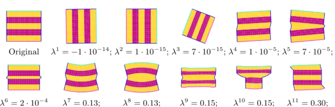
Original λ1
= −1 · 10−14; λ2= 1 · 10−15; λ3= 7 · 10−15; λ4= 1 · 10−5; λ5= 7 · 10−5;
λ6
= 2 · 10−4 λ7= 0.13; λ8= 0.13; λ9= 0.15; λ10= 0.15; λ11= 0.30;
Fig. 1.Original configuration and first eleven eigenvectors for a floating subdomain. With K = 0.1 we select six eigenvectors for the projection space. Among these, the first three correspond to the rigid body modes ( ˜Ajp
1,2,3
j = 0). In total the size of the
projection space is 46.
In this section for lack of space we have chosen to illustrate the way that the method works rather than a set of performance tests. The implementation uses matlab and Freefem++. We solve the two dimensional linear elasticity equations
discretized with P1(piecewise linear) finite elements on a 121× 16 regular mesh
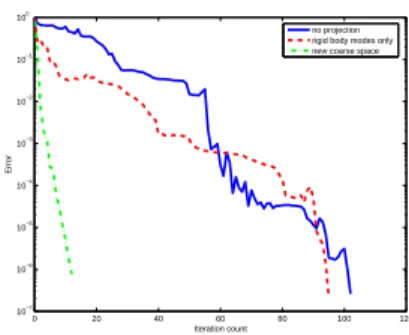
8 Nicole Spillane 0 20 40 60 80 100 120 10−7 10−6 10−5 10−4 10−3 10−2 10−1 100 Iteration count Error no projection rigid body modes only new coarse space
Fig. 2. Error versus the iteration count for three methods: no projection (blue full line), projection onto the rigid body modes (red hashes), projection onto the space from definition 1 (green hashes and dots). The new projections space does its job. The condition number is reduced from 3576 to 13. With just the rigid body modes it is 1808.
into 8 side by side unit squares. Then we add one layer of overlap to each. The
medium is a soft material (Lam´e parameters: E = 107, ν = 0.4) with two layers
of a harder material (E = 1012, ν = 0.4). In Figure 4 we have plotted the original
configuration for one subdomain as well as the first eigenmodes for eigenproblem (12). In Figure 4 we show that the new method converges very fast and that the projection step does its job since it reduces the condition number from 3576 to 13 using only 46 projection vectors.
References
1. Z. Dost`al, Conjugate gradient method with preconditioning by projector, Interna-tional Journal of Computer Mathematics, 23(3-4), 315-323, 1988.
2. Y. Saad, Iterative methods for sparse linear systems, SIAM, 2003.
3. N. Spillane, D. Rixen Spectral coarse spaces for robust FETI and BDD algorithms, in preparation, 2012.
4. A. Toselli, O. Widlund Domain decomposition methods: algorithms and theory, Springer, 2005.
5. M. Brezina, C. Heberton, J. Mandel, P. Vanˇek, An iterative method with con-vergence rate chosen a prioriTechnical Report 140, University of Colorado Denver, CCM, University of Colorado Denver, April 1999.
6. Y. Efendiev, J. Galvis and R. Lazarov, J. Willems, Robust domain decomposi-tion precondidecomposi-tioners for abstract symmetric positive definite bilinear forms, ESAIM, 46(05):11751199, 2012.
7. N. Spillane, V. Dolean, P. Hauret, F. Nataf, C. Pechstein, R. Scheichl, A Robust Two Level Domain Decomposition Preconditioner for Systems of PDEs, Comptes Rendus Math´ematique, 349(23-24):12551259, 2011.
8. N. Spillane, V. Dolean, P. Hauret, F. Nataf, C. Pechstein, R. Scheichl, Abstract Robust Coarse Spaces for Systems of PDEs via Generalized Eigenproblems in the Overlaps, NuMa-Report, 2011-07, 2007.