Aligning capital with risk

(1)

Aligning Capital with Risk

A dissertation presented by

Silvan Ebnöther

Supervised by

Prof. Fabio Trojani

Prof. Roberto Ferretti

Prof. Paolo Vanini

Submitted to the

Faculty of Economics

Università della Svizzera italiana

for the degree of

Ph.D. in Economics

(2)

PhD$Thesis) )

Aligning)Capital)with)Risk)

) Silvan)Ebnöther) Università)della)Svizzera)italiana) ) September)10,)2015) ) The)interaction)of)capital)and)risk)is)of)primary)interest)in)the)corporate)governance)of)banks)as) it)links)operational)profitability)and)strategic)risk)management.)Kaplan)and)Norton)(1992))noted) that) senior) executives) understand) that) their) organization’s) monitoring) system) strongly) affects) the) behaviour) of) managers) and) employees.) Typical) instruments) used) by) senior) executives) to) focus) on) strategy) are) balanced) scorecards) with) objectives) for) performance) and) risk) management,) including) an) according) payroll) process.) A) top$down) capital$at$risk) concept) gives) the) executive) board) the) desired) control) of) the) operative) behaviour) of) all) risk) takers.) It) guarantees)uniform)compensations)for)business)risks)taken)in)any)division)or)business)area.)The) standard) theory) of) cost$of$capital) (see) e.g.) Basel) Committee) on) Banking) Supervision) (2009))) assumes) standardized) assets.) Return) distributions) are) equally) normalized) to) a) one$year) risk) horizon.)It)must)be)noted)that)risk)measurement)and)management)for)any)individual)risk)factor) has) a) bottom$up) design.) The) typical) risk) horizon) for) trading) positions) is) 10) days,) 1) month) for) treasury)positions,)1)year)for)operational)risks)and)even)longer)for)credit)risks.)My)contribution) to)the)discussion)is)as)follows:)In)the)classical)theory,)one)determines)capital)requirements)and) risk) measurement) using) a) top$down) approach,) without) specifying) market) and) regulation) standards.)In)my)thesis)I)show)how)to)close)the)gap)between)bottom$up)risk)modelling)and)top$ down)capital)alignment.)I)dedicate)a)separate)paper)to)each)risk)factor)and)its)application)in)risk) capital)management.))

)

Risk%factor% Operational%risk% Credit%risk% Market%risk%

Type%of%business% Workflows)and)systems) Lending) Treasury) Trading)

Cause%of%loss% Failed)processes;)people) and)systems) Defaults)of)counterparties) Interest)rate)and) liquidity)risks) Price)and) volatility)risks) Countermeasures% Checks)and)balances) including)separation)of) competence;)) project)planning)and) management)process) Counterparty)validation) and)rating)processes;) standardized)lending) process;) credit)limit)management) Maturity) matching;) hedge)accounting;) cash)flow) modelling) Discipline,) continuous) hedging)with) risk) constraints)

Risk%horizon% Yearly) Multi$year) Monthly) 10)days)

Risk;alignment%to% annual%planning% process% In)line,)i.e.)no)scaling) needed) Down$scaling)of)long$term) risk)to)one$year) Up$scaling)of)short)term)risk)to) one$year)) Literature%about% risk%measurement% Little)literature)on) operational)risk) measurement)(and) predominant)loss)data) analysis)) Lots)of)literature)about) credit)risk)modelling;)no) literature)on)down$scaling) Lots)of)literature)about)modelling,) pricing)and)hedging,)probability) processes)and)empirical)studies) Contribution%of%my% thesis% Link)between)operational) workflows)and) operational)risk) measurement) Multi$year)modelling)with) down)scaling)to)a)one$ year)horizon)and)linking) to)risk)capital) Discussion)and)guidance)of)up) scaling)short$term)risk)measures)to) a)one$year)horizon)and)linking)to) risk)capital) Table%1:%Risk%factors%and%their%different%characteristics%for%risk%capital%management%%

(3)

The) cumulative) thesis) consists) of) four) individual) scholarly) papers.) Three) papers) embrace) the) annual)budgeting)of)risk)capital)for)(i))operational)risk,)(ii))credit)risk,)and)(iii))market)risk.)The) fourth)contribution)uses)game)theory)for)analysing)the)allocation)of)an)open)line)of)credit)to)an) entrepreneur.) • Silvan)Ebnöther,)Paolo)Vanini,)Alexander)McNeil,)Pierre)Antolinez)(2003):)Operational) Risk:)A)Practitioner's)View,)Journal)of)Risk,)5)(3),)pp.)1$16.)(NCCR)Working)Paper)No.)52)) • Silvan)Ebnöther,)Paolo)Vanini)(2007):)Credit)portfolios:)What)defines)risk)horizons)and) risk)measurement?,)Journal)of)Banking)and)Finance,)31)(12),)pp.)3663$3679.)(NCCR) Working)Paper)No.)221)) • Silvan)Ebnöther,)Markus)Leippold,)Paolo)Vanini)(2006):)Optimal)credit)limit) management)under)different)information)regimes,)Journal)of)Banking)and)Finance,)30) (2),)pp.)463$487.)(NCCR)Working)Paper)No.)72))

• Silvan) Ebnöther) (2015),) Economic) capital) for) market) risk,) Working) Paper,) Available) at) Social)Science)Research)Network)(papers.ssrn.com))

Operational%risk:%A%practitioner's%view%

In) June) 1999,) the) Basel) Committee) on) Banking) Supervision) (’’the) Committee’’)) released) its) consultative) document) ’’The) New) Basel) Capital) Accord’’) (’’The) Accord’’)) that) proposed) a) regulatory) capital) charge) to) cover) ’’other) risks’’.) The) operational) risk) is) one) such) ’’other) risk) factor’’.)Since)the)publication)of)the)document)and)its)sequels,)the)industry)and)the)regulatory) authorities)have)been)engaged)in)vigorous)and)recurring)discussions.)The)banking)industry)has) reached) a) better) understanding) and) offered) a) more) precise) definition) of) operational) risk.) By) now,) the) topic) of) operational) risks) is) dealt) with) in) a) more) process) oriented) way.) However,) in) practice,)operational)risks)are)subject)to)a)qualitative)rather)than)quantitative)approach.)Hardly) any) papers) have) studied) the) quantitative) modelling) of) operational) risks.) The) few) quantitative) papers)available)propose)to)collect)loss)data)and)to)apply)extreme)value)theory)on)the)datasets.)) I) contribute) to) these) debates) from) a) practitioner’s) point) of) view.) To) achieve) this,) I) consider) a) number)of)issues)of)operational)risk)from)a)case)study)perspective.)The)case)study)is)defined)for) a) bank's) production) unit) and) factors) in) self$assessment) as) well) as) historical) data.) The) results) show)that)I)can)define)and)model)operational)risk)for)workflow)processes.)More)specifically,)if) operational) risk) is) modelled) on) well$defined) objects,) all) vagueness) is) dispelled) although) compared) with) market) or) credit) risk,) a) different) methodology) and) different) statistical) techniques) are) used.) An) important) insight) from) a) practitioner’s) point) of) view) is) that) not) all) processes) in) an) organization) need) to) be) equally) considered) for) the) purpose) of) accurately) defining) operational) risk) exposure.) The) management) of) operational) risks) can) focus) on) key) issues;) a) selection) of) the) relevant) processes) significantly) reduces) the) costs) of) defining) and) designing) the) workflow) items.) In) a) next) step,) the) importance) of) the) four) risk) factors) system) failure,)theft,)fraud)and)error)is)analysed)using)compound)Poisson)processes)and)extreme)value) theory)technics.)While)for)quality)management)all)factors)matter,)fraud)and)system)failure)have) a)non$reliable)impact)on)risk)figures.)Finally,)I)am)able)to)link)risk)measurement)to)the)needs)of) risk)management.)) Credit%portfolios:%What%defines%risk%horizons%and%risk%measurement?% In)this)part)of)the)thesis,)I)describe)the)setup)and)calibration)of)a)multi$period)credit)portfolio) model)and)how)to)achieve)risk)figures)which)are)in)line)with)a)one$year)bank)policy.)) The)strong)autocorrelation)between)economic)cycles)demands)that)I)analyse)credit)portfolio)risk) in)a)multiperiod)setup.)I)embed)a)standard)one$factor)model)in)such)a)setup.)To)be)more)precise,)

(4)

I)work)with)a)synthetic)Merton$type)one$factor)model)in)which)the)obligor’s)future)rating)grade) depends)on)its)synthetic)asset)value,)which)is)itself)a)linear)combination)of)one)systematic)and) one)idiosyncratic)factor.)I)discuss)the)calibration)of)the)one$period)model)to)Standard)&)Poor’s) ratings)data)in)detail)and)use)a)maximum)likelihood)method)as)proposed)by)Gordy)and)Heidfeld) (2002).)I)extend)the)model)to)a)multi$period)setup)by)estimating)an)implicit)realization)path)of) the) systematic) factor.) The) idea) of) inversely) calculating) a) realization) path) was) also) applied) in) Belkin) et) al.) (1998).) But,) I) use) only) historical) default) rates) for) our) calibration) to) achieve) consistency) to) the) “through$the$cycle”) rating) definition) used) by) rating) agencies.) I) calibrate) a) simple) time) series) model) to) this) realization) path.) The) results) show) a) significantly) positive) autocorrelation.)This)multi$year)extension)of)the)credit)portfolio)model)exactly)captures)the)time) dependence)structure)of)the)assumed)default)statistic.)

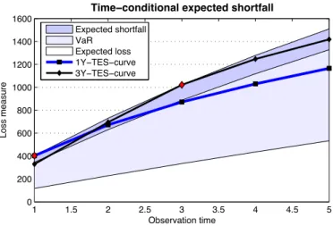
Because)single$period)risk)measures)cannot)capture)the)cumulative)effects)of)systematic)shocks) over) several) periods,) I) define) an) alternative) risk) measure,) which) I) call) the) time$conditional) expected) shortfall) (TES),) to) quantify) credit) portfolio) risk) over) a) multiperiod) horizon.) This) measure)extends)expected)shortfall.)Simulating)a)portfolio)similar)to)the)S&P)portfolio,)I)show) that)using)TES)as)a)risk)measure,)a)bank)can)achieve)enough)capital)cushions)to)cover)losses)in) credit$risky)portfolios)if)heavy)losses)in)a)given)year)are,)as)they)most)probably)are,)followed)by) comparable) losses) in) the) subsequent) years) due) to) the) autoregressive) behaviour) of) business) cycles.)

Optimal%credit%limit%management%under%different%information%regimes%

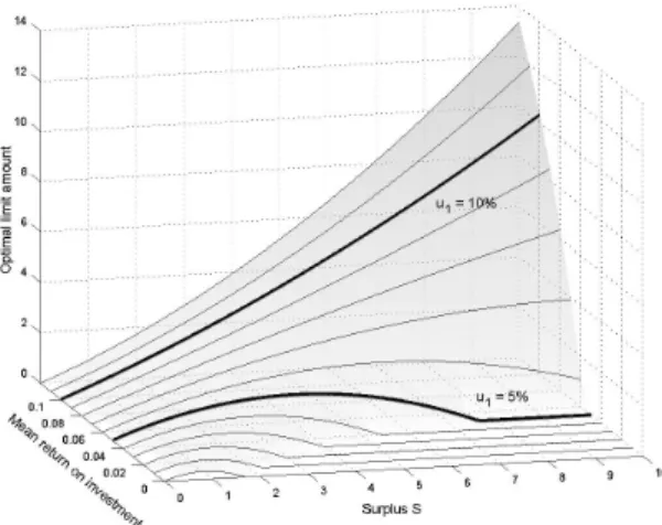
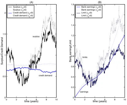
Credit) limit) management) is) of) paramount) importance) for) successful) short$term) credit$risk) management,) even) more) so) when) the) situation) in) credit) and) financial) markets) is) tense.) By) focusing)on)limit)management,)we)illuminate)an)aspect)of)credit)risk)modelling)different)from) the) traditional) approaches) initiated) by) Merton) (1974)) and) Black) and) Cox) (1976).) I) consider) a) continuous$time)model)where)the)credit)provider)and)the)credit)taker)interact)within)a)game$ theoretic)framework)under)different)information)structures.)From)a)modelling)point)of)view,)I) assume) that) the) risk) and) return) characteristics) of) the) debtor’s) investment) process) affect) the) bank’s) limit) assessment) decision) at) any) given) time.) The) demand) for) credit) following) from) the) optimality)of)the)debtor’s)investment)decision)defines)an)earning)component)in)the)bank’s)value) function.) In) turn,) the) bank’s) limit) assessment) affects) the) optimization) problem) of) the) firm) by) bounding) the) possible) credit) exposure.) Therefore,) the) analysis) of) credit) limit) management) is) defined) as) the) solution) of) a) dynamic) non$cooperative) game.) This) setup) relates) the) proposed) model) to) the) theory) of) differential) games,) first) introduced) in) Isaacs) (1954).) In) particular,) the) model)comes)close)to)the)continuous$time)model)in)Holmström)and)Milgrom)(1987),)where)one) agent) controls) the) drift) rate) vector) of) a) multi$dimensional) Brownian) motion.) However,) the) presented) model) differs) in) the) underlying) information) structure.) In) addition) to) incomplete) information)on)the)firm’s)actions,)the)model)features)partial)information)on)the)state)variable.) Furthermore,)the)debtor’s)credit)decision)influences)both)drift)and)variance)of)the)surplus.)The) model) with) complete) information) provides) decision$theoretic) insights) into) the) problem) of) optimal) limit) policies) and) motivates) more) complicated) information) structures.) Moving) to) a) partial) information) setup,) incentive) distortions) emerge) that) are) not) in) the) bank’s) interest.) I) discuss)how)these)distortions)can)effectively)be)reduced)by)an)incentive$compatible)contract.)

Economic%capital%for%market%risk)

Market)risk)results)from)trading)and)treasury)positions.)The)effective)risk)horizons)for)traders) and)treasurers)are)less)than)one)year.)It)is)not)reasonable)for)market)risk)positions)to)measure) their)risk)on)a)one$year)horizon)due)to)the)implicit)assumption)that)traders)or)treasurers)hold) theirs) portfolios) constant) up) to) the) risk) horizon.) Since) they) are) continuously) adapting) and)

(5)

hedging)their)portfolios)due)to)market$shifts,)they)redeploy)their)trading)positions)and)treasury) exposures)several)times)during)a)year.)Nevertheless,)risk)capital)charges)must)base)on)a)single) enterprise$wide)risk)horizon)that)must)not)coincide)with)the)risk)factor)specific)horizons.)The) proposed) risk) consumption) approach) brings) these) different) views) between) (i)) risk) measurement) and) management) on) a) short$term) horizon) and) (ii)) risk) capital) on) a) long$term) horizon)in)line.))

In) this) part) of) the) thesis,) I) present) a) new) approach) that) I) have) not) encountered) in) any) other) scholarly) papers.) I) put) forward) and) analyse) an) idea) of) risk) budgeting) that) leads) back) to) discussions) with) Thomas) Domenig,) a) former) risk) manager) at) Zurich) Cantonal) Bank.) A) bank) assigns) an) annual) risk) budget) to) its) market) risk) managers.) The) annual) risk) budget) equals) the) probability)of)an)annual)loss)higher)than)a)predefined)capital$at$risk.)Throughout)the)year,)the) budget) that) the) risk) manager) consumes) is) greater) the) higher) the) risk) he) takes.) His) risk) consumption)equates)the)probability)of)a)year$to$date)loss)in)excess)of)the)capital$at$risk)at)the) 10$day) risk) horizon.) As) soon) as) the) risk) manager) has) completely) consumed) his) annual) risk) budget,)he)immediately)has)to)hedge)his)positions.) References) Selected)literature)to)cost)of)capital)and)balanced)scorecard) • Robert)S.)Kaplan)and)David)P.)Norton)(1992),)The)balanced)scorecard:)measures)that)drive) performance,)Harvard)Business)Review,)January$February)1992.) • Franco)Modigliani)and)Merton)H.)Miller)(1958),)The)cost)of)capital,)corporate)finance)and) the)theory)of)investment,)The)American)Economic)Review,)48)(3):)216$297,)June)1958.) • Basel)Committee)on)Banking)Supervision)(2009),)Range)of)practices)and)issues)in) economic)capital)modeling,)Bank)for)International)Settlements,)Basel.) ) Operational)Risk:)A)Practitioner's)View) • Embrechts,)P.,)C.)Klüppelberg)and)T.)Mikosch)(1997),)Modelling)Extremal)Events)for) Insurance)and)Finance,)Springer,)Berlin.)) • Lindskog,)F.)and)A.J.)McNeil)(2001),)Common)Poisson)Shock)Models,)Applications)to) Insurance)and)Credit)Risk)Modelling,)Preprint,)ETH)Zürich.)) • Medova,)E.)(2000),)Measuring)Risk)by)Extreme)Values,)Operational)Risk)Special)Report,) Risk,)November)2000.)) ) Credit)portfolios:)What)defines)risk)horizons)and)risk)measurement?) • Allen,)L.)and)Saunders,)A.:)2003,)A)survey)of)cyclical)effects)in)credit)risk)measurement) models,)BIS)working)papers)(126).) • Belkin,)B.,)Forest,)L.)and)Suchower,)S.:)1998,)A)one$parameter)representation)of)credit)risk) and)transition)matrices,)CreditMetrics)Monitor,)Third)Quarter)1998)pp.)46–56.) • Gagliardini,)P.)and)Gouriéroux,)C.:)2005,)Stochastic)migrations)models)with)application)to) corporate)risk,)Journal)of)Financial)Econometrics)3(2),)188–226.) • Gordy,)M.)and)Heitfield,)E.:)2002,)Estimating)default)correlations)from)short)panels)of) credit)rating)performance)data,)Federal)Reserve)Board)Working)Paper).) • Löffler,)G.:)2004,)An)anatomy)of)rating)through)the)cycle,)Journal)of)Banking)&)Finance) 28(3),)695–720.)) • Merton,)R.)C.:)1974,)On)the)pricing)of)corporate)debt:)The)risk)structure)of)interest)rates,) The)Journal)of)Finance)29(2),)449–70.)) • Trück,)S.)and)Rachev,)S.)T.:)2005,)Credit)portfolio)risk)and)probability)of)default)confidence) sets)through)the)business)cycle,)The)Journal)of)Credit)Risk)1(4).) )

(6)

Optimal)credit)limit)management)under)different)information)regimes) • Anderson,)R.)and)Sundaresan,)S.:)1996,)Design)and)valuation)of)debt)contract,)Review)of) Financial)Studies)9(1),)37–68.) • Black,)F.)and)Cox,)J.:)1976,)Valuing)corporate)securities:)Some)effects)of)bond)indenture) provision,)Journal)of)Finance)31(2),)351–367.) • Grossman,)S.)and)Hart,)O.:)1983,)An)analysis)of)the)principal$agent)problem,)Econometrica) 51(1),)7–45.) • Holmström,)B.)and)Milgrom,)P.:)1987,)Aggregation)and)linearity)in)the)provision)of) intertemporal)incentives,)Econometrica)55,)303–328.) • Isaacs,)R.:)1954,)Differential)games,)i,)ii,)iii,)iv,)Reports)rm$1931,)1399,)1411,)1486,)Rand) Corporation.) • Kalman,)R.:)1960,)A)new)approach)to)linear)filtering)and)prediction)problems,)Journal)of) Basic)Engineering)82,)35–45.) • Leland,)H.:)1994,)Corporate)debt)value,)bond)covenants,)and)optimal)capital)structure,) Journal)of)Finance)49,)1213–1252.) • Lintner,)J.:)1956,)Distribution)of)incomes)of)corporations)among)dividends,)retained) earnings,)and)taxes,)American)Economic)Review)46,)7113.) • Mirrless,)J.:)1971,)An)exploration)in)the)theory)of)optimum)income,)Review)of)Economic) Studies)38,)175–208.) ) Economic)capital)for)market)risk) • H.)J.)Blommestein,)L.)H.)Hoogduin,)and)J.)J.)W.)Peeters.)Uncertainty)and)risk)management) after)the)great)moderation:)The)role)of)risk)(mis)management)by)financial)institutions.) Paper)for)the)28th)SUERF)Colloquium)on)’The)quest)for)stability’,)Utrecht,)The) Netherlands,)2009.) • Domenig,)T.,)Ebnöther,)S.)and)Vanini,)P.:)2005,)Aligning)capital)with)risk,)Risk)Day)2005,) Center)of)Competence)Finance)in)Zurich)) • Leo)Grepin,)Jonathan)Tétrault,)and)Greg)Vainberg.)After)black)swans)and)red)ink:)How) institutional)investors)can)rethink)risk)management.)McKinsey)Working)Papers)on)Risk,) (17),)2010.) • Grant)Kirkpatrick.)Corporate)governance)lessons)from)the)financial)crisis.)Financial) Market)Trends,)1(96),)2009.) • OECD.)Corporate)governance)and)the)financial)crisis:)Key)findings)and)main)massages.) June)2009.) • Francesco)Saita.)Risk)Capital)Aggregation:)The)Risk)Manager’s)Perspective.)EFMA)2004) Basel)Meetings)Paper,)2004.) ) )

(7)

(8)

2SHUDWLRQDO⇤5LVN ⇤$⇤3UDFWLWLRQHU⌦V⇤9LHZ⇤

By Silvan Ebnöther

a

, Paolo Vanini

b

Alexander McNeil

c

, and Pierre Antolinez

d

a

Corporate Risk Control, Zürcher Kantonalbank, Neue Hard 9, CH-8005 Zurich,

e-mail: silvan.ebnoether@zkb.ch

b_{Corresponding author,}

Institute of Finance, University of Southern Switzerland, CH-6900 Lugano, e-mail: paolo.vanini@zkb.ch

c

Department of Mathematics, ETH Zurich, CH-8092 Zurich, e-mail: alexander.mcneil@math.ehtz.ch

d

e-mail: pierre.antolinez@zkb.ch

(9)

2SHUDWLRQDO⇤5LVN Version: October 11, 2002 2

$EVWUDFW⇤

The Basel Committee on Banking Supervision ("the Committee") released a consultative document that included a regulatory capital charge for operational risk. Since the release of the document, the complexity of the concept of "operational risk" has led to vigorous and recurring discussions. We show that for a production unit of a bank with well-defined workflows operational risk can be unambiguously defined and modelled. The results of this modelling exercise are relevant for the implementation of a risk management framework, and the pertinent risk factors can be identified. We emphasize that only a small share of all workflows make a significant contribution to the resulting VaR. This result is quite robust under stress testing. Since the definition and maintenance of processes is very costly, this last result is of major practical importance. Finally, the approach allows us to distinguish features of quality and risk management respectively.

.H\ZRUGV Operational Risk, Risk Management, Extreme Value Theory, VaR -(/⇤&ODVVLILFDWLRQ ⇤&⌧✏⇤&⇡⌧✏⇤* ✏⇤* ⇤⇤

$FNQRZOHGJHPHQW ⇤:H⇤DUH⇤HVSHFLDOO\⇤JUDWHIXO⇤WR⇤3URIHVVRU⇤(PEUHFKWV⇤↵(7+ ⇤IRU⇤KLV⇤SURIRXQG⇤LQVLJKWV⇤ DQG⇤ QXPHURXV⇤ YDOXDEOH⇤ VXJJHVWLRQV⌘⇤ :H⇤ DUH⇤ DOVR⇤ JUDWHIXO⇤ WR⇤ $⌘⇤ $OOHPDQQ✏⇤ 8⌘⇤ $PEHUJ✏⇤ 5⌘⇤ +RWWLQJHU⇤ DQG⇤ 3⌘⇤ 0HLHU⇤ IURP⇤ =ÅUFKHU⇤ .DQWRQDOEDQN⇤ IRU⇤ SURYLGLQJ⇤ XV⇤ ZLWK⇤ WKH⇤ GDWD⇤ DQG⇤ UHOHYDQW⇤ SUDFWLFDO⇤ LQVLJKW⌘⇤ :H⇤ ILQDOO\⇤ WKDQN⇤ WKH⇤ SDUWLFLSDQWV⇤ RI⇤ WKH⇤ VHPLQDUV⇤ DW⇤ WKH⇤ 8QLYHUVLWLHV⇤ RI⇤ 3DYLD✏⇤ /XJDQR⇤ DQG⇤ =XULFK⇤ DQG⇤ WKH⇤ ,%0⇤ ◆◆ ⇤ )LQDQFH⇤ )RUXP✏⇤ =XULFK⌘⇤ 3DROR⇤ 9DQLQL⇤ ZRXOG⇤ OLNH⇤ WR⇤ WKDQN⇤ WKH⇤ 6ZLVV⇤ 1DWLRQDO⇤6FLHQFH⇤)RXQGDWLRQ⇤↵1&&5⇤),15,6. ⇤IRU⇤WKHLU⇤ILQDQFLDO⇤VXSSRUW⌘

(10)

⇤ ,QWURGXFWLRQ⇤

In June 1999, the Basel Committee on Banking Supervision (’’the Committee’’) released its consultative document ’’The New Basel Capital Accord’’ (’’The Accord’’) that included a proposed regulatory capital charge to cover ’’other risks’’. Operational risk (OR) is one such ’’other risk’’. From the time of the release of this document and its sequels (BIS (2001)), the industry and the regulatory authorities have been engaged in vigorous and recurring discussions. It is fair to say that at the moment, as far as operational risk is concerned the "Philosopher’s Stone" is yet to be found.

Some of the discussions are on a rather general and abstract level. For example, there is still ongoing debate concerning a general definition of OR. The one adopted by the BIS Risk Management Group (2001) is ’’the risk of direct loss resulting form inadequate or failed internal processes, people and systems or from external events.’’ How to translate the above definition into a capital charge for OR has not yet been fully resolved; see for instance Danielsson et al. (2001). For the moment, legal risk is included in the definition, whereas systemic, strategic and reputational risks are not.

The present paper contributes to these debates from a practitioner’s point of view. To achieve this, we consider a number of issues of operational risk from a case study perspective. The case study is defined for a bank's production unit and factors in self-assessment as well as historical data. We try to answer the following questions quantitatively:

1. Can we define and model OR for the workflow processes of a bank's production unit (production processes)? A production process is roughly a sequence of business activities; a definition is given in the beginning of Section 2.

2. Is a portfolio view feasible and with what assets? 3. Which possible assessment errors matter?

4. Can we model OR such that both the risk exposure and the causes are identified? In other words, not only risk measurement but risk management is the ultimate goal.

5. Which are the crucial risk factors?

6. How important is comprehensiveness? Do all workflows in our data sample significantly contribute to the operational risk of the business unit?

The results show that we can give reasonable answers to all the questions raised above. More specifically, if operational risk is modelled on well-defined objects, all vagueness is dispelled although compared with market or credit risk, a different methodology and different statistical techniques are used. An important insight from a practitioner’s point of view is that not all processes in an organization need to be equally considered for the purpose of accurately defining operational risk exposure. The management of operational risks can focus on key issues; a selection of the relevant processes significantly reduces the costs of defining and designing the workflow items. To achieve this goal, we construct the Risk Selection Curve (RiSC), which singles out the relevant workflows needed to estimate the risk figures. In a next step, the importance of the four risk factors considered is analyzed. As a first result, the importance of the risk factors depends non-linearly on the confidence level used in measuring risk. While for quality management all factors matter, fraud and system failure have a non-reliable impact on risk figures. Finally, with the proposed methodology we are able to link risk measurement to the needs of risk management: For each risk tolerance level of the management there exists an appropriate risk measure. Using this measure RiSC and the risk factor contribution anaylsis select the relevant workflows and risk factors.

The paper is organized as follows. In Section 2 we describe the case study. In Section 3 the results using the data available are discussed and compared for the two models. Further, some important issues raised by the case study are discussed. Section 4 concludes.

(11)

⇤ &DVH⇤6WXG\⇤

The case study was carried out for Zürcher Kantonalbank's Production Unit. The study comprises 103 production processes.

⌘⇤ 0RGHOOLQJ⇤2SHUDWLRQDO⇤5LVN ⇤)UDPHZRUN⇤

The most important and difficult task in the quantification of operational risk is to find a reasonable model for the business activities1. We found it useful, for both practical and theoretical reasons, to think of quantifiable operational risk in terms of directed graphs. Though this approach is not strictly essential in the present paper, for operational risk management full-fledged graph theory is crucial (see Ebnöther et al. (2002) for a theoretical approach). In this paper, the overall risk exposure is considered on an aggregated graph level solely for each process. This approach of considering first an aggregated level is essential from a practical feasibility point of view: Considering the costly nature of analyzing the operational risk of processes quantitatively on a "microscopic level", the important processes have to be selected first.

In summary, each workflow is modelled as a graph consisting of a set of nodes and a set of directed edges. Given this skeleton, we next attach risk information. To this end, we use the following facts: At each node (representing, say, a machine or a person) errors in the processing can occur (see Figure 1 for an example).

⇤

,QVHUW⇤)LJXUH⇤⇤DURXQG⇤KHUH⌘⇤

The errors have both a cause and an effect on the performance of the process. More precisely, at each node there is a (random) input of information defining the performance. The errors then affect this input to produce a random output performance. The causes at a node are the risk factors, examples being fraud, theft or computer system failure. The primary objective is to model the link between effects and causes. There are, of course, numerous ways in which such a link can be defined. As operational risk management is basically loss management, our prime concern is finding out how causes, through the underlying risk factors, impact losses at individual edges.

We refer to the entire probability distribution associated with a graph as the RSHUDWLRQV⇤ ULVN⇤ GLVWULEXWLRQ. In our modelling approach, we distinguish between this distribution and RSHUDWLRQDO⇤ULVN⇤ GLVWULEXWLRQ. While the operations risk distribution is defined for all losses, the operational risk distribution considers only losses larger than a given WKUHVKROG.

Operational risk modelling, as defined by the Accord, corresponds to the operations risk distribution in our setup. In practice, this identification is of little value as every bank distinguishes between small and large losses. While small losses are frequent, large losses are very seldom encountered. This implies that banks know a lot about the small losses and their causes but they have no experience with large losses. Hence, typically an efficient organization exists for small losses. The value added of quantitative operational risk management for banks thus lies in the domain of large losses (low intensity, high severity). This is the reason why we differentiate between operations risk and operational risk LI quantitative modelling is considered. We summarize our definition of operational risk as follows:

'HILQLWLRQ⇤4XDQWLWDWLYH⇤RSHUDWLRQDO⇤ULVN⇤IRU⇤D⇤VHW⇤RI⇤SURGXFWLRQ⇤SURFHVVHV⇤DUH⇤WKRVH⇤RSHUDWLRQV⇤ULVNV⇤ ZKLFK⇤H[FHHG⇤D⇤JLYHQ⇤WKUHVKROG⇤YDOXH⌘

Whether or not we can use graph theory to calculate operational risk critically depends on the existence of VWDQGDUGL]HG⇤ DQG⇤ VWDEOH workflows within the banking firm. The cost of defining

1_{Strictly speaking there are three different objects: Business activities, workflows, which are a first model of these activities, and graphs,}

which are a second model of business activities based on the workflows. Loosely speaking, graphs are mathematical models of workflows with attributed performance and risk information relevant to the business activities. In the sequel we use business activities and workflows as synonyms.

(12)

processes within a bank can be prohibitively large (i) if all processes need to be defined, (ii) if they are defined on a very deep level of aggregation, or (iii) if they are not stable over time.

⌘ ⇤ 'DWD⇤

An important issue in operational risk is data availability. In our study we use both self-assessment and historical data. The former are based on H[SHUW⇤NQRZOHGJH. More precisely, the respective process owner valued the risk of each production process. To achieve this goal, standardized forms were used where all entries in the questionnaire were properly defined. The experts had to assess two random events:

1. The frequency of the random time of loss. For example, the occurrence probability of an event for a risk factor could be valued ’’high/medium/low’’ by the expert. By definition the ’’medium’’ class might, for example, comprise one-yearly events up to four-yearly events. 2. The experts had to estimate maximum and minimum possible losses in their respective

processes. The assumed severity distribution derived from the self-assessment is calibrated using the loss history2_{. This procedure is explained in chapter 2.4.}

If we use expert data, we usually possess sufficient data to fully specify the risk information. The disadvantage of such data concerns their quality. As Rabin (1998) lucidly demonstrates in his review article, people typically fail to apply the mathematical laws of probability correctly but instead create their own ’’laws’’ such as the ’’law of small numbers’’. An expert based database thus needs to be designed such that the most important and prominent biases are circumvented and a sensitivity analysis has to be done. We therefore represented probabilistic judgments in the case study unambiguously as a choice among real life situations.

We found three principles especially helpful in our data collection exercise: 1. 3ULQFLSOH⇤, Avoid direct probabilistic judgments.

2. 3ULQFLSOH⇤ ,, Choose an optimal interplay between experts’ know how and modelling. Hence the scope of the self-assessment has to be well defined. Consider for example the severity assessment: A possible malfunction in a process leads to losses in the process under consideration. The same malfunction can also affect other workflows within the bank. Experts have to be awake to whether they adopt a local point of view in their assessment or a more global one. In view of the pitfalls inherent in probabilistic judgments, experts should be given as narrow a scope as possible. They should focus on the simplest estimates, and model builders should perform more complicated relationships based on these estimates.

3. 3ULQFLSOH⇤,,, ⇤Implement the right incentives. In order to produce the best result it is important not only to advise the experts on what information they have to deliver, but also to make it clear why it is beneficial for them and the whole institution to do so. A second incentive problem concerns accurate representation. Specifically, pooling behavior should be avoided. By and large, the process experts can be classified in three categories at the beginning of a self-assessment: Those who are satisfied with the functioning of their processes, those who are not satisfied with the status but have so far been unable to improve their performance and, finally, experts who well know that their processes should be redesigned but have no intention of doing so. For the first type, making an accurate representation would not appear to be a problem. The second group might well exaggerate the present status to be worse than it in fact is. The third group has an incentive to mimic the first type. Several measures are possible to avoid such pooling behavior, i.e. having other employees crosscheck the assessment values, and comparing with loss data where available. And ultimately, common sense on the part of the experts’ superiors can reduce the extent of misspecified data due to pooling behavior.

2

(13)

The historical data are used for calibration of the severity distribution (see Section 2.4). At this stage, we restrict ourselves to noting that information regarding the severity of losses is confined to the minimum/maximum loss value derived from the self-assessment.

⌘ ⇤ 7KH⇤0RGHO⇤

Within the above framework, the following steps summarize our quantitative approach to operational risk:

1. First, data are generated through simulation starting from expert knowledge.

2. To attain more stable results, the distribution for large losses is modelled using extreme value theory.

3. Key risk figures are calculated for the chosen risk measures. We calculate the VaR and the conditional VaR (CVaR)3.

4. A sensitivity analysis is performed.

Consider a business unit of a bank with a number of production processes. We assume that for workflow i there are 4 relevant risk factors Ri,j, j = 1,..., 4, leading to a possible process malfunction

such as system failure, theft, fraud, or error. Because we do not have any experience with the two additional risk factors external catastrophes and temporary loss of staff, we have not considered them in our model. In the present model we assume that all risk factors are LQGHSHQGHQW.

To generate the data, we have to simulate two risk processes: The stochastic time of a loss event occurrence and the stochastic loss amount (the severity) of an event expressed in a given currency. The number Ni,j of workflow i malfunctions by risk factor j and the associated severity Wi,j(n), n =

1,...Ni,j, are derived from expert knowledge. Ni,j is assumed to be a homogeneous Poisson process.

Formally, the inter-arrival times between successive losses are i.i.d, exponentially distributed with finite mean 1/li,j. The parameters li,j are calibrated to the expert knowledge database.

The severity distributions Wi,j (n) ~ Fi,j, for n=1, … , Ni,j are estimated in a second step. The

distribution of severity Wi,j(n) is modeled in two different ways. First, we assume that the severity is a

combined Beta and generalized Pareto distribution. In the second model, a lognormal distribution is used to replicate the severity.

If the (i,j)-th loss arrival process Ni,j (t), t s 0, is independent from the loss severity process

{Wi,j(n)}n N and Wi,j(n) has the same distribution for each n and are independent, then the total loss

experienced by process i due to risk type j up to time t

∑

= = ) ( 1 , , , ) ( ) (W : Q 6

is called a compound Poisson process. We always simulate 1 year. For example, 10,000 simulations of S(1) means that we simulate the total first years loss 10,000 times.

The next step is to specify the tail of the loss distribution as we are typically interested in heavy losses in operational risk management. We use extreme value theory to smooth the total loss distribution. This theory allows a categorization of the total loss distribution into different qualitative tail regions4. In summary, Model 1 is specified by:

3

VaR denotes the Value-at-Risk measure and CVaR denotes Conditional Value-at-Risk (CVaR is also called Expected Shortfall or Tail Value-at-Risk (See Tasche (2002)).

4_{We consider the mean excess function e}

1(u) = E[S(1)-u | S(1) u] for 1 year, which by our definition of operational risk is a useful

measure of risk. The asymptotic behavior of the mean excess function can be captured by the generalized Pareto distribution (GPD) G. The GPD is a two-parameter distribution with distribution function

      = − − ≠ + − = − , 0 if ) exp( 1 , 0 if ) 1 ( 1 ) ( 1 , ξ σ ξ σ ξ ξ σ ξ

where > 0 and the support is [0, ) when 0 and [0,- / ] for < 0. A good data fit is achieved which leads to stable results in the calculation of the conditional Value-at-Risk (see Section 3).

(14)

• Production processes which are represented as aggregated, directed graphs consisting of two nodes and a single edge,

• Four independent risk factors,

• A stochastic arrival time of loss events modelled by a homogeneous Poisson process and the severity of losses modeled by a Beta-GPD-mixture distribution. Assuming independence, this yields a compound Poisson model for the aggregated losses.

• It turns out that the generalized Pareto distribution, which is fitted by the POT5 method, yields an excellent fit to the tail of the aggregate loss distribution.

• The distribution parameters are determined using maximum likelihood estimation techniques. The generalized Pareto distribution is typically used in extreme value theory. It provides an excellent fit to the simulated data for large losses. Since the focus is not on choosing the most efficient statistical method, we content ourselves with the above choice while being very aware that other statistical procedures might work equally well.

⌘⌫⇤ &DOLEUDWLRQ⇤

Our historical database6 contains losses that can be allocated to the workflows in the production unit. We use this data to calibrate the severity distribution, noting that the historical data show an expected bias: Due to the relevance of operational risk in the last years, more small losses are seen in 2000 and 2001 than in previous years.

For the calibration of the severity distribution we use our loss history and the assessment of the maximum possible loss per risk factor and workflow. The data are processed in two respects. First, as the assessment of the minimum is not needed since it is used for accounting purposes only, we drop this number. Second, errors may well lead to losses instead of gains. In our database a small number of such gains occur. Since we are interested solely in losses, we do not consider events leading to gains.

Next we observe that the maximum severity assessed by the experts is exceeded in some processes. In our loss history, this effect occurs with an empirical conditional probability of 0.87% per event. In our two models, we factor this effect into the severity value by accepting losses higher than the maximum assessed losses.

Calibration is then performed as follows:

• We first allocate each loss to a risk factor and to a workflow.

• Then we normalize the allocated loss by the maximum assessed loss for its risk factor and workflow.

• Finally we fit our distribution to the generated set of normalized losses. It follows that the lognormal distribution and a mixture of the Beta and generalized Pareto distribution provide the best fits to the empirical data.

In the second simulation, we have to multiply the simulated normalized severity by the maximum assessed loss to generate the loss amount (reversion of the second calibration step).

⌘⌫⌘⇤ /RJQRUPDO⇤0RGHO⇤

In our first model of the severity distribution, we fit a lognormal distribution to the standardized losses.

The lognormal distribution seems to be a good fit for the systematic losses. However, we observe that the probability of occurrence for large losses is greater than the empirical data show.

5

The Peaks-Over-Threshold (POT) method based on a GPD model allows construction of a tail fit above a certain threshold u; for details of the method, see the papers in Embrechts (2000).

(15)

⌘⌫⌘ ⇤ %HWD⇣*3'⇣0L[WXUH⇤0RGHO⇤

We eliminate the drawbacks of the lognormal distribution by searching for a mixture of distributions which satisfies the following properties:

First, the distribution has to reliably approximate the normalized empirical distribution in the domain where the mass of the distribution is concentrated. The flexibility of the Beta distribution is used for fitting in the interval between 0 and the estimated maximum Xmax.

Second, large losses, which probably exceed the maximum of the self-assessment, are captured by the GPD with support the positive real numbers. The GPD distribution is estimated using all historical normalized losses higher than the 90% quantile. In our example, the relevant shape parameter x of the GPD fit is nearly zero, i.e. the distribution is medium tailed7. To generate the losses, we choose the exponential distribution which corresponds to a GPD with x=0.

Our Beta-GPD-mixture distribution is defined by a combination of the Beta- and the Exponential distribution. A Beta-GPD-distributed random variable X satisfies the following rules: With probability p, X is a Beta random variable, and with probability (1-p), X is a GPD-distributed random variable. Since 0.87% of all historical data exceed the assessed maximum, the weight p is chosen such that P(X > Xmax) = 0.87% holds.

The calibration procedure reveals an important issue if self-assessment and historical data are considered: Self-assessment data typically need to be processed if they are compared with historical data. This shows that the reliability of the self-assessment data is limited and that by processing this data, consistency between the two different data sets is restored.

⇤ 5HVXOWV⇤

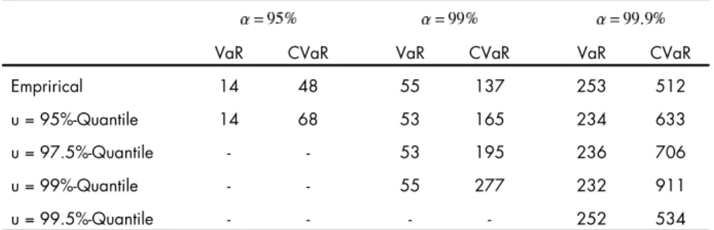
The data set for the application of the above approaches is based on 103 production processes at Zürcher Kantonalbank and self-assessment of the probability and severity of losses for four risk factors (see Section 2.1). The model is calibrated against an internal loss database. Since confidentiality prevents us from presenting real values, the absolute values of DOO results are fictitious but the relative magnitudes are real. The calculations are based on 10,000 simulations. Table 1 shows the results for the Beta-GPD-mixture model.

VaR CVaR VaR CVaR VaR CVaR

Emprirical 17 41 60 92 134 161

u = 95%-Quantile 17 55 52 129 167 253

u = 97.5%-Quantile - - 59 10 133 165

u = 99%-Quantile - - 60 91 132 163

u = 99.5%-Quantile - - - - 134 161

7DEOH⇤  Simulated data behavior of the tail distribution. ’’Empirical’’ denotes the results

derived from 10,000 simulations for the Beta-mixture model. The other key figures are generated using the POT8 model for the respective thresholds u.

Using the lognormal model to generate the severities the VaR for a = 95% and 99% respectively are approximately the same. The lognormal distribution is more tailed than the Beta-GPD-mixture distribution that leads to higher key figures for the 99.9% quantile.

7

The lognormal model bellows to the medium tailed distributions, too. But we observe that the tail behavior of the lognormal distribution converts very slowly to = 0. For this reason, we anticipate that the resultant distribution on the yearly total loss will seem to be heavily tailed. Only a large-scale simulation could observe this fact.

8

From Table 1 and 2 it follows that the POT model yields a reasonable tail fit. For further information on the underlying loss tail behavior and statistical uncertainty of the estimated parameters we refer to Ebnöther (2001).

(16)

Emprirical 14 48 55 137 253 512

u = 95%-Quantile 14 68 53 165 234 633

u = 97.5%-Quantile - - 53 195 236 706

u = 99%-Quantile - - 55 277 232 911

u = 99.5%-Quantile - - - - 252 534

7DEOH⇤ Simulated data behavior of the tail distribution. Instead of the Beta-mixture

model of Table 1 the lognormal model is used for the severity.

We can observe that a robust approximation of the coherent risk measure CVaR is more sensitive to the underlying loss distribution. The Tables also confirm that the lognormal model is more heavily tailed than the Beta-mixture model.

⌘⇤ 5LVN⇤6HOHFWLRQ⇤&XUYH⇤

A relevant question for practitioners is how much each of the processes contributes to the risk exposure. If it turns out that only a fraction of all processes significantly contribute to the risk exposure, then risk management needs only to be defined for these processes.

We therefore analyze how much each single process contributes to the total risk. We consider only VaR in the sequel as a risk measure. To split up the risk into its process components, we compare the risk contributions (RC) of the processes.

Let RC (i) be the risk contribution of process i to VaR at the confidence level a }) { \ ( VaR ) ( VaR ) ( RC L = 3 − 3 L ,

where P is the whole set of workflows.

Because the sum over all RC ’s is generally not equal to the VaR, the relative risk contribution (RRC ) (i) of process i is defined as the RC (i) normalized by the sum over all RC , i.e.

∑

− = = M L 3 3 M L L ) ( RC }) { \ ( VaR ) ( VaR ) ( RC ) ( RC ) ( RRC .

As a further step, for each a, we count the number of processes that exceed a relative risk contribution of 1%. We call the resulted curve with parameter a, the Risk Selection Curve (RiSC).

,QVHUW⇤)LJXUH⇤ ⇤DURXQG⇤KHUH⌘⇤

Figure 2 shows that on a reasonable confidence level only about 10 percent of all processes contribute to the risk exposure. Therefore only for this small number of processes is it worth developing a full graph theoretical model and analyzing this process in more detail. On lower or even low confidence levels, more processes contribute to the VaR. This indicates that there are a large number of processes of the high frequency/low impact type. These latter processes can be singled out for quality management, whereas processes of the low frequency/high impact type are under the responsibility of risk management. In summary, using RiSC graphs allows a bank to discriminate between quality and risk management in respect of the processes which matter. This reduces costs for both types of management significantly and indeed renders OR management feasible.

We finally note that the shape of the RiSC, i.e. not monotone decreasing, is not a product of modelling.

From a risk management point of view RiSC links the measurement of operational risk to its management as follows: Each parameter value a represents a risk measure and therefore, in Figure 2

(17)

on the horizontal axes a family of risk measures is shown. The risk managers possess a risk tolerance that can be expressed with a specific value a. Hence, RiSC provides the risk information managers are concerned with.

⌘ ⇤ 5LVN⇤)DFWRU⇤&RQWULEXWLRQ⇤

The information concerning the most risky processes is important for splitting the Value at Risk into its risk factors. Therefore we determine the relative risk that a risk factor contributes to the VaR in a similar manner to the former analysis. We define the relative risk factor contribution as

∑

= − − = ₄ 1 })) { \ ( VaR (VaR }) { \ ( VaR VaR ) ( RRFC M 3 L 3 L ,

with P now the whole set of risk factors.

The resultant graph clearly shows the importance of the risk factors. ,QVHUW⇤)LJXUH⇤ ⇤DURXQG⇤KHUH⌘

Figure 3 shows that the importance of the risk factors is not uniform and in linear proportion to the scale of confidence levels. For low levels, error is the most dominant factor, which again indicates that this domain is best covered by quality management. The higher the confidence level is, the more fraud becomes the dominant factor. The factor theft displays an interesting behavior too: It is the sole factor showing a virtually constant contribution in percentage terms at all confidence levels.

Finally, we note that both results, RiSC and the risk factor contribution, were not known to the experts in the business unit. These clear and neat results contrast with the diffuse and disperse knowledge within the unit about the risk inherent in their business.

⌘ ⇤ 0RGHOOLQJ⇤'HSHQGHQFH⇤

In the previous model we assumed the risk factors were independent. Dependence could be introduced though a so-called common shock model (see Bedford and Cooke (2001), Chapter 8, and Lindskog and McNeil (2001)). A natural approach to model dependence is to assume that all losses can be related to a series of underlying and independent shock processes. When a shock occurs, this may cause losses due to several risk factors triggered by that shock.

We did not implement dependence in our case study for the following reasons:

• The occurrence of losses which are caused by fraud, error and theft are independent.

• While we are aware of system failures dependencies, these are not the dominating risk factor. (See figure 3.) Hence, the costs for an assessment and calibration procedure are too large compared to the benefit of such an exercise.

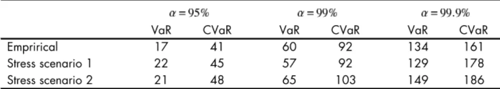
⌘⌫⇤ 6HQVLWLYLW\⇤$QDO\VLV⇤

We assume that for each workflow and each risk factor the estimated maximum loss is twice the self-assessed value, and then twice that value again. In doing so, we also take into account that the calibration to the newly generated data has to be redone.

Emprirical 17 41 60 92 134 161

Stress scenario 1 22 45 57 92 129 178

Stress scenario 2 21 48 65 103 149 186

7DEOH⇤ Stress scenario 1 is a simulation using a maximum twice the self-assessed value.

Stress scenario 2 is a simulation using a maximum four times the self-assessed value. A Beta-GPD-mixture distribution is chosen as severity model.

(18)

It follows that an overall underestimation of the estimated maximum loss does not have a significant effect on the risk figures since the simulation input is calibrated to the loss history.

Furthermore, the relative risk contributions of the risk factors and processes do not change

significantly under these scenarios, i.e. the number of processes which significantly contribute to the VaR remains almost invariant and small compared to all processes.9

⌫⇤ &RQFOXVLRQ⇤

The scope of this paper was to show that quantification of operational risk (OR), adapted to the needs of business units, is feasible if data exist and if the modelling problem is seriously considered. This means that the solution of the problem is described with the appropriate tools and not by an ad hoc deployment of methods successfully developed for other risks.

It follows from the results presented that a quantification of OR and OR management must be based on well-defined objects (processes in our case). We do not see any possibility of quantifying OR if such a structure is not in place within a bank. It also follows that not all objects (processes for example) need to be defined; if the most important are selected, the costs of monitoring the objects can be kept at a reasonable level and the results will be sufficiently precise. The self-assessment and historical data used in the present paper proved to be useful: applying a sensitivity analysis, the results appear to be robust. In the derivation of risk figures we assumed that risk tolerance may be non-uniform in the management. Therefore, risk information is parameterized such that the appropriate level of confidence can be chosen.

The models considered in this paper can be extended in various directions. First, if the Poisson models used are not appropriate, they can be replaced by a negative Binomial process (see Ebnöther (2001) for details). Second, production processes are only part of the total workflow processes defining business activities. Hence, other processes need to be modelled and using graph theory a comprehensive risk exposure for a large class of banking activities is derived.

9

(19)

⇠⇤ 5HIHUHQFHV⇤

• BIS 2001, Basel Committee on Banking Supervision (2001), Consultative Document, The New Basel Capital Accord, http://www.bis.org.

• BIS, Risk Management Group of the Basel Committee on Banking Supervision (2001), Working Paper on the Regulatory Treatment of Operational Risk, http://www.bis.org.

• Bedford, T. and R Cooke (2001), Probabilistic Risk Analysis, Cambridge University Press, Cambridge.

• Danielsson J., P. Embrechts, C. Goodhart, C. Keating, F. Muenich, O. Renault and H. S. Shin (2001), An Academic Response to Basel II, Special Paper Series, No 130, London School of Economics Financial Markets Group and ESRC Research Center, May 2001

• Ebnöther, S. (2001), Quantitative Aspects of Operational Risk, Diploma Thesis, ETH Zurich. • Ebnöther, S., M. Leippold and P. Vanini (2002), Modelling Operational Risk and Its

Application to Bank's Business Activities, Preprint.

• Embrechts, P. (Ed.) (2000), Extremes and Integrated Risk Management, Risk Books, Risk Waters Group, London

• Embrechts, P., C. Klüppelberg and T. Mikosch (1997), Modelling Extremal Events for Insurance and Finance, Springer, Berlin.

• Lindskog, F. and A.J. McNeil (2001), Common Poisson Shock Models, Applications to Insurance and Credit Risk Modelling, Preprint, ETH Zürich.

• Medova, E. (2000), Measuring Risk by Extreme Values, Operational Risk Special Report, Risk, November 2000.

• Rabin, M. (1998), Psychology and Economics, Journal of Economic Literature, Vol. XXXVI, 11-46, March 1998.

• Tasche, D. (2002), Expected Shortfall and Beyond, Journal of Banking and Finance 26(7), 1523-1537.

(20)

2SHUDWLRQDO⇤5LVN Version: October 11, 2002 13 (GLW⇤⇣⇤SRVW⇤UHWXUQ Modelling Modelling e 1 = < k 1 , k 2 > e 2₌ < k 2 , k 3 > e 3 = < k 3 , k 4 > e 4 = < k 4 , k 5 > e₅ = < k₂ , k₆ > e 1 = < k 1 , k 2 > k₂ k₁ k₃ k₄ k₅ k₆ Business unit B Envelope to the account executive Business unit B New envelope Send a new correspondence Business unit B Same address

Check the address on system X Business unit B Yes No Accept a post-return Business unit A k₂ k₁ ∼ ~ ~ ~ ~ ~

)LJXUH⇤  Example of a simple production process: The edit-post return. More

complicated processes can contain several dozens of decision and control nodes. The graphs can also contain loops and vertices with several legs, i.e. topologically the edit - post process is of a particularly simple form. In the present paper, condensed graphs (Model 1) are only considered, while for risk management purposes the full graphs are needed.

(21)

(22)

(23)

(24)

Credit portfolios: What defines risk

horizons and risk measurement?

⇤

Silvan Ebn¨

other

University of Southern Switzerland, CH-6900 Lugano,

Z¨urcher Kantonalbank, Josefstrasse 222, CH-8005 Zurich,

e-mail: silvan.ebnoether@zkb.ch

Paolo Vanini

Swiss Banking Institute, University of Z¨urich, CH-8032 Z¨urich,

Z¨urcher Kantonalbank, Josefstrasse 222, CH-8005 Zurich,

e-mail: paolo.vanini@zkb.ch

First version: August 2005

This version: Monday 13

th

November, 2006

Abstract

The strong autocorrelation between economic cycles demands that we analyze credit portfolio risk in a multiperiod setup. We embed a standard one-factor model in such a setup. We discuss the calibration of the model to Standard & Poor’s ratings data in detail. But because single-period risk measures cannot capture the cumulative e↵ects of systematic shocks over several periods, we define an alternative risk measure, which we call the time-conditional expected shortfall (TES), to quantify credit portfolio risk over a multiperiod horizon.

JEL Classification Codes: C22, C51, E22, G18, G21, G33.

Key words: Credit risk management, portfolio management, risk measurement, coherence, VaR, expected shortfall, factor model

⇤_{Silvan Ebn¨other and Paolo Vanini acknowledge the financial support of Zurich Cantonal Bank}

(ZKB), and Swiss National Science Foundation (NCCR FINRISK) respectively. Corresponding author: Paolo Vanini.

(25)

Monday 13th _{November, 2006} _{Credit portfolios: What defines risk horizons and risk measurement?}

1 Introduction

Banks typically measure credit risk over a one-year time horizon, using either value-at-risk (VaR) or expected shortfall (ES) as measures of risk. We claim that the risk horizon has to be longer than one year, because derived risk capital must cover all but the worst possible losses in a credit portfolio. If there is a longer time horizon, then the key risk factor for huge portfolio losses is the economic cycle, which we must model autoregressively. We further extend the standard one-period value-at-risk and shortfall-risk measures to meet the requirements of a multiperiod context. Several facts support these claims. First, although the length, depth, and di↵usion of recessions or even de-pressions has varied significantly in the past, it turns out that a one-year time horizon is often too short to account for a business cycle. For example, when we use the National Bureau of Economic Research (NBER) definition of recessions and depressions, we see that in the U.S. economy for the last 200 years, deep recessions lasted between 35 and 65 months. These long-standing recessions suggest that we should measure credit risk over longer than one year. We believe that a five-year time horizon might be appropriate. We could calculate the risk on a one-year basis and - assuming independence - scale the figures to five years. The reason we do not do so is the autocorrelation in the business cycle: if the industry does badly this year, the probability that it does even worse in the next year is higher than the probability of a strong upwards move. Such an auto-correlation of the business cycle must be accounted for in the risk measurement, else we will underestimate risk in periods of economic downturns. The autocorrelated behavior requires a multiperiod view. The analysis below, which uses Standard & Poor’s (S&P)

default statistics1_{, strongly supports the claim that autocorrelation matters.}

Business cycles and factors that are specific to the credit business determine the risk horizon. For example, if we use a risk measure in market risk, then we assume a holding period of ten days with fixed portfolio fractions. There are at least two reasons why such an assumption is useful. First, to try to foresee how portfolios are rebalanced in the future is not realistic. Second, a possible extreme scenario is that trading in a specific period is not, or is almost not, possible. For example, if the liquidity due to a shock event evaporates. Therefore, the risk horizon should also roughly convey during which time changes in the positions are not possible. Two properties define this time for credit risk. First, di↵erent types of loan contracts have di↵erent maturities and options for exiting and recontracting. Basel II assumes a mean time to maturity of 2.5 years. We can qualitatively confirm this figure if we calculate the mean time of maturity for a portfolio of approximatively 20,000 counterparties. Second, the ability of the institution to buy/sell credit risk on secondary markets is important. The stronger a firm’s ability to trade on secondary markets, the shorter the risk’s time horizon. These considerations lead us to conclude that that it does not suffice to measure the credit risk of long-term credit investments on a one-year risk horizon. Moreover, based on the significant au-tocorrelation of default rates, a bank that holds only enough capital to cover one-year

1_{We use public Standard & Poor’s data in our case study. The data are described in detail in}

Standard & Poor’s ratings performance 2003, see Standard & Poor’s (2004).

(26)

losses does not possess enough financial substance to cover multiyear recessions. There-fore, we suggest a credit horizon equal to the maturity of a credit. Since model risk increases with longer risk horizons, it is reasonable to assume a maximal model horizon. We choose a five-year model horizon.

Having established the need for a multiperiod model and a risk horizon longer than a one year, we explain why we need a revision of the usual risk measures. Since we model risk in a multiperiod way, we must define the risk measure for more than one future date. That is, we must show that cumulative losses at di↵erent dates in the risk measure lead to meaningful measures of risk. To put it another way, we show that in a multiperiod setup, value-at-risk or expected shortfall underestimate the loss potential in a credit-risky portfolio. We define a new risk measure, which we call time-conditional expected shortfall (TES). TES possesses our required properties. First, it accounts for the fact that heavy credit risk losses can occur in consecutive years. Therefore, TES provides enough capital cushions to survive such events. Second, TES is an extension of expected shortfall and therefore is easily calculated as this one-period risk measure. The paper is organized as follows. Since our multiperiod model extends a single period

one, in Section 2 we reconsider the industry standard one-period, one-factor

Merton-type credit risk model. Section3extends the model to several periods, i.e., we consider

the single economic factor in the Merton model in a multiperiod horizon. Section 4

considers risk measurement in a multiperiod setting. Section5 concludes.

2 One-period model

We work with a synthetic Merton-type one-factor model in which the obligor’s future

rating grade depends on its synthetic asset value2_{, which is itself a linear combination}

of one systematic and one idiosyncratic factor. Each rating grade is associated with a specified range of obligor’s asset value.

Risk management uses factor models for various reasons. First, these models allow us to integrate economic variables. Second, calibration is a standard routine. Third, the models are applicable to internal ratings, since they can be generalized to arbitrary rating definitions and rating grades. Hence, they can be used for small- and medium-sized firms, which represent the majority of counterparties for most institutions. Finally, the Basel Committee also suggests a one-factor model.

Gupton, Finger and Bhatia (1997) and Belkin, Forest and Suchower (1998) show in-depth analysis of one-period factor models and their calibration.

2.1 The model

To summarize factor models, we consider a discrete set of ratings _{R = {1, ..., N}R}. We

define NR as the default grade, Rit 2 R as the rating grade of obligor i = 1, ..., Nobl at

(27)

time t, and Mi

t(r, s) =P Rti = s|Rit 1 = r as the transition probability that obligor i

will migrate from rating r to rating s between t 1 and t.

A single firm defaults as per definition of Merton (1974) if its asset value Ai

t falls below a

critical threshold of liability di_{. Factor models extend this idea to portfolios of obligors.}

We use a standard one-factor model to define the portfolio behavior on a one-year risk horizon. The asset value of an obligor is the weighted sum of its joint systematic factor and its idiosyncratic risk factor. That is, the creditworthiness and rating migration

prob-abilities of all obligors depend on one single economic factor, Zt. This key assumption

characterizes the dependence structure between the default probabilities of obligors. Assumption 2.1. Comparability and dependency

Migration probabilities for firms with the same rating grade r are equal. The di↵erence in migration probabilities for each rating grade and scenario depends only on the realization of the market factor Z.

We next formalize the relation between default/migration probabilities and the economic

factor Z. When we define the synthetic asset return Ai

t of obligor i as a linear

combina-tion of the systematic factor Zt and its idiosyncratic risk "it with systematic weight !,

we have:

Ai_t := !Zt+

p

1 !2_"i

t, (1)

where we assume that Z, ✏ follow a independent standard normal distribution, i.e.,

Zt, "it ⇠ N (0, 1) (i.i.d). (We note that we use the shorthand Z, "i for Zt, "it in the

one-period setup.) We associate to each rating grade r a range of the asset value.

Obligor i with initial rating r at time t 1 has rating s at time t if Ai

t 2 [✓r,s+1, ✓r,s).

The thresholds ✓r,s2 R satisfy

1 = ✓r,1 ✓r,2 ... ✓r,s ... ✓r,NR ✓r,NR+1 = 1. (2)

We set dr := ✓r,NR for the default thresholds. The thresholds follow from the calibration.

Then the migration probabilities of obligor i with initial rating r are

Mi

t(r, s) = P Rit= s|Rit 1= r

= P Ai_t2 [✓r,s+1, ✓r,s) . (3)

Since the synthetic asset returns in equation (1) are still standard normally distributed,

the Z-conditional expected default rate of rating grade r reads:

pr(Z) = dr !rZ p 1 !2 r ! (4)

with (·) as the cumulative standard normal distribution function.

(28)

2.2 Calibration

We calibrate the one-period one-factor model to historical Standard & Poor’s data, see

Standard & Poor’s (2004). To achieve this goal, we must fix the thresholds ✓r,s and the

correlation parameters !r for all r and s. We use a two-step estimation. First, we fix

the threshold values such that the resulting transition probability matrixM matches the

empirical matrix M. In the second step, we estimate the risk weights !r, for all r2 R.

We calibrate the migration matrixM is calibrated by dividing the number of firms with

rating s at the end of a period by the number of firms with initial rating r, i.e.,

Mr,s =

P

t] Obligors with rating r at time t_P 1 and rating s at time t

t] Obligors with rating s at time t 1

. (5)

The number of S&P-rated companies increases from 1,371 companies in 1981 to 5,322 companies in 2003. We exclude firms that S&P has not rated (N.R.) at the end of the year. Since there are no registered defaults for the S&P best rating grade AAA, we also exclude AAA firms from our analysis. Furthermore, there is only a single

default event for a AA firm. Then the estimated AA default probability p2 = 0.01%

and the variance var(p2) =

p

p2(1 p2)/9756 = 0.01% are similar for a sample size

of 9,756. Hence, results based on this AA statistic have to be adequately considered. The estimated variances for other rating grades are acceptable. The standard normal

assumption of the synthetic asset returns implies the calibration condition M(r, s) =

(✓r,s) (✓r,(s+1)). Hence, we fix the default threshold dr = ✓r,Nr =

1_(p

r) and than

calculate the remaining thresholds as

✓r,s= 1(M(r, s) + (✓r,(s+1))) (6)

for s = NR 1 to s = 2.

Although the expected loss depends only on exposure and default probabilities, portfolio risk is highly sensitive to the correlation parameter !. A sophisticated calibration of ! is more ambitious and di↵erent procedures are used in practice, see Gupton et al. (1997), Gordy (2000), Gordy and Heitfield (2002) and Gagliardini and Gouri´eroux (2005). A major reason for the difficulty is the short rating-time series. The S&P ratings report, which we use in our calibration, contains a sufficient sample to estimate plausible

cor-relations !r for all r 2 R. The easiest and fastest estimation procedure is the moment

matching method (MM). We summarize this approach in AppendixA. Gordy and

Heit-field (2002) argue that although moment matching methods are common, they often lead to only crude estimations. They propose to use not only some moment statistics, but the whole available data set. A maximum likelihood method promises better estimates, al-though, due to limited data, this approach can also produce biased parameter estimates.

We use the maximum likelihood method to calibrate the correlations !. Let Nr and Dr

denote the number of obligors and the number of defaults in rating grade r. Equation

(29)

default probability pr := pr(Z) = pr(Z|!r), the number of defaults Dr in a sample of

size Nr follows a binomial distribution with likelihood

L(Dr, Nr|pr) = ✓ Nr Dr ◆ pDr r (1 pr)Nr Dr. (7)

The unconditional likelihood of the factor model follows by integrating over the market factor Z: L(D, N) = EZ " Y r2R L (Dr, Nr|pr(Z|!r)) # (8) = Z R Y r2R ✓✓ Nr Dr ◆ pr(Z|!r)Dr(1 pr(Z|!r))Nr Dr ◆ d (Z).

We next apply equation (8) to the S&P sample from 1981 to 2003. The maximum

likelihood estimation ! of vector ! is

! = arg max !2[ 1,1]NR Y year ti Y r2R L(Dti,r, Nti,r|!r) (9) = arg max !2[ 1,1]NR Y year ti Z R Y r2R ✓✓ Nti,r Dti,r ◆ pr(Zti|!r) D_ti,r₍₁ _p r(Zti|!r)) N_ti,r D_ti,r ◆ d (Zti).

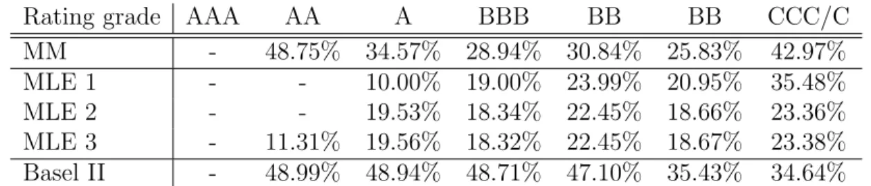
Table 1 summarizes the resulting weights !r, for all r 2 R. Instead of estimating the

Rating grade AAA AA A BBB BB BB CCC/C

MM - 48.75% 34.57% 28.94% 30.84% 25.83% 42.97%

MLE 1 - - 10.00% 19.00% 23.99% 20.95% 35.48%

MLE 2 - - 19.53% 18.34% 22.45% 18.66% 23.36%

MLE 3 - 11.31% 19.56% 18.32% 22.45% 18.67% 23.38%

Basel II - 48.99% 48.94% 48.71% 47.10% 35.43% 34.64%

Table 1: The table shows rating-specific risk weights calibrated to historical default rates of S&P. Since S&P does not register defaults are for AAA companies, we cannot estimate the economic risk factor for such companies. We also doubt the significance for the AA grade, since there is only one default. We use the following abbreviations: MM for moment matching, MLE 1 for five independent estimations for the five weights

!A, ..., !CCC, MLE 2 for one estimation for the five weights, and MLE 3 for one

estima-tion for six weights.

default probabilities p = (p1, ..., pNr) and the systematic weights ! = (!1, ..., !Nr) in

two separate steps, we also solve the maximization problem (9) in a single step. See

Appendix B for the results, which are comparable to those described in the two-step

procedure.