GEOMAGIA50.v3: 1. general structure and modifications to the archeological and volcanic database

(1)

User’s Guide to GEOMAGIA50.v3:

1. Archeomagnetic and Volcanic Database

Maxwell C. Brown1,∗, Fabio Donadini2, Monika Korte1, Andreas Nilsson3,4, Kimmo Korhonen5, Alexandra Lodge3,6, Stacey N. Lengyel7 and Catherine G. Constable8

1_{GFZ German Research Centre for Geosciences, Telegrafenberg, 14473, Potsdam, Germany}

2_{Department of Earth Sciences, University of Fribourg, Chemin du Mus´}_{ee 6, 1700 Fribourg, Switzerland}

3_{Geomagnetism Laboratory, Department of Earth, Ocean and Ecological Sciences, University of Liverpool, Liverpool, L69 7ZE,}

UK

4_{Current address: Department of Geology, Quaternary Sciences, Lund University, S¨}_{olvegatan 12, 223-62 Lund, Sweden} 5_{Geological Survey of Finland (GET), P.O. Box 96 (Betonimiehenkuja 4), FI-02151 Espoo, Finland}

6_{Current address: AWE Blacknest, Brimpton, Reading, RG7 4RS, UK}

7_{Illinois State Museum, Research and Collections Center, 1011 E. Ash Street, Springﬁeld, Illinois, USA}

8_{Institute of Geophysics and Planetary Physics, Scripps Institution of Oceanography,University of California, San Diego, La}

Jolla, CA 92092-0225, USA

∗_{Contact at}_{mcbrown@gfz-potsdam.de}

T

his guide constitutes the additional ﬁle for Brown et al. (2015a), hereafter re-ferred to as B15a.

List of Figures

S1 Query form . . . 2 S2 General constraints panel . . . 4 S3 Geographic constraints panel . . . . 6

S4 Magnetic data results table . . . 8 S5 Downloads tab . . . 9 S6 Google visualization . . . 10

List of Tables

S1 Magnetic results table . . . 14 S2 Radiocarbon age results table . . . . 15 S3 Model output table . . . 15

1 Guide to the function of the

archeomagnetic and volcanic

web page

1.1 Archeomagnetic and volcanic query form

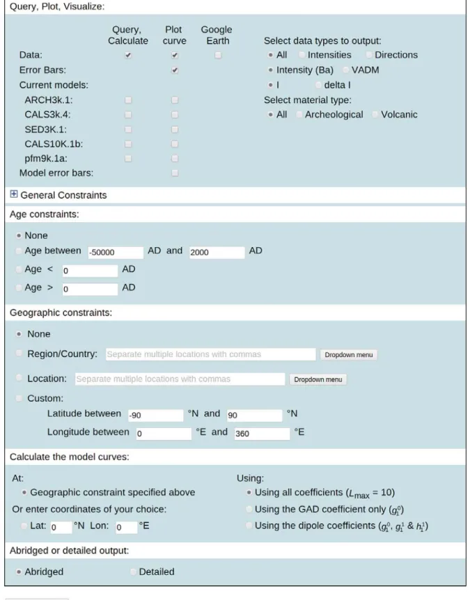
The archeomagnetic and volcanic query form (Fig. S1) can be accessed at http://geomagia.

gfz-potsdam.de/geomagiav3/AAquery.php or through the ‘Archeomagnetic and volcanic query form’ link in the left navigation menu. The main functions of this form are brieﬂy described, proceeding from the top of the form down.

1.1.1 Query, Plot, Visualize

Archeomagnetic and volcanic data are requested to query, view online and download by selecting the checkbox under ‘Query, Calculate’. Selecting the

(2)

Figure S1: Initial state of the archeomagnetic and volcanic query form after the user has selected the ‘Archeomagnetic and volcanic query form’ link from the left navigation menu on the GEOMAGIA50 home page or entered

(3)

checkbox below ‘Plot curve’ will generate a series of plots on the ‘Figures and Downloads’ tab (sec-tion 1.2), which can be downloaded. The ‘Query, Calculate’, ‘Plot curve’ and ‘Error Bars’ checkboxes are automatically selected on loading the web page. Deselecting the ‘Plot curve’ checkbox increases the speed of the query and is useful when performing a reconnaissance of the database. When the ‘Er-ror Bars’ checkbox is selected, uncertainties on age and paleomagnetic data are plotted. Uncertainties are shown by default in the ‘Query results’ table under the ‘Magnetic data’ tab and in the .CSV ﬁle available to download (section 1.2). Selecting the ‘Google Earth’ checkbox will activate a Google Earth plug-in on the ‘Google Visualization’ tab enabling the user to see site information and results from a .kml ﬁle (section ‘Google visualization’ in B15a and section 1.2).

The type of paleomagnetic data shown in the ‘Query results’ table under the ‘Magnetic data’ tab (section 1.2), the .CSV file available to download, plotted and included in the model output file can be refined by selecting radio buttons under ‘Select data types to output’ on the right-hand side of the ‘Query, Plot, Visualize’ panel. There are three rows

of radio buttons.

The top row allows the selection of all paleomag-netic data or a choice between paleointensities and directions. Only the relevant columns are output. In the second row either paleointensity (Ba) or VADM will be output (section ‘Query, plot, visualize’ in B15a). In the third row either inclination (‘I’) or in-clination anomaly (‘delta I’) can be selected (section ‘Query, plot, visualize’ in B15a). Lastly, the ‘Select material type’ radio buttons allow the user to limit the output data to either archeological or volcanic. By default the ‘All’ radio button is selected. This option is new in version 3 of the database.

In the lower portion of the panel the location de-pendent output from five models (section 2) can be queried and plotted by selecting checkboxes in the same way as for the archeomagnetic and vol-canic data. A bootstrap estimate uncertainty en-velope can be plotted for all models (with the ex-ception of pfm9k.1a) by selecting the ‘Model error bars’ check box. On executing the query, plots and plain text files are created and can be downloaded via links on the download page (section 1.2). Un-certainties are automatically shown in the .TXT file containing the model outputs (section 1.2); the er-ror bars check box is not required to be selected. For all models, age and geographic constraints are set in ‘Age constraints’ (section 1.1.3), ‘Geographic

constraints’ (section1.1.4) or ‘Calculate the model curves’ (section1.1.5). Model data are not queried if a geographic constraint is not given or if more than one country/region or location entered. If custom latitudes and longitudes are selected in geographic constraints, the mid-point coordinates will be used in the output calculation. If the user desires they can alternatively calculate inclination as inclination anomaly (ΔI) and intensity as VADM. See Table S3 for descriptions of the column headers used in the model output ﬁles. The model output can be reﬁned further in the ‘Calculate the model curves’ panel (section1.1.5).

1.1.2 General constraints

General constraints are initially concealed when the archeomagnetic and volcanic query form loads. They can be accessed by clicking on the plus sign to the left of ‘General constraints’. This reveals an additional panel on the query form (Fig.S2). The panel is split into ﬁve sections: (1) ‘Material’; (2) ‘PI Method’; (3) ‘Dating Method’; (4) ‘Specimen Type’; and (5) ‘Site statistics’. Within a section there are a selection of checkboxes, more than one of which can be checked at the same time. The options checked in each section are activated by selecting the checkboxes next to the section name and again more than one section can be activated at the same time.

The user can select as many check boxes as desired in each panel and options from all ﬁve panels can be selected at once if desired. Options within the panels act as ’or’ statements, e.g., if two options are selected then only data from one of the options needs exist to return a result, not both. An exception is in the ‘PI Method’ panel. In this panel, between rows are ‘or’ statements, and within a row, but between columns are ‘and’ statements, with the exception of ‘Other parameters’, where between ‘Anisotropy’ and ‘NRM parallel to NRM’ is logically an ‘or’ statement. Be-tween all other options in ‘Other parameters’ lie ‘and’ statements. Additionally, between options within one column of a row in the PI panel are ‘or’ statements. For all other panels, if multiple panels are selected then ‘and’ statements exist between the panel op-tions, e.g., if ‘Ceramic’ is selected from the ‘Material’ panel and ‘Shaw’ is selected from the ‘PI Method’ panel, only data obtained using the Shaw (1974) paleointensity method on ceramics will be returned. If options inside a section are selected but the checkbox next to the section name is not, the options will not be added to the database query and all data will be returned which match any other constraints

(4)

(5)

selected; however, a warning message will appear in the general constraints box in the ‘Summary of query parameters’ table on the ‘Magnetic data’ tab (section1.2) and the user will be asked to select the checkbox next to the relevant section name (if they desire). The checkboxes next to section names can be useful when a large number of checkboxes within a section have been selected, yet the user wishes not to use these options, but does not want to deselect every checkbox. Instead, the user can deselect the checkbox next to the section name and the options within the section will be ignored. This is useful when options within more than one section have been selected and a user wishes to compare the database output when diﬀerent constraints are applied. In addition, it makes reactivating a large number of options eﬃcient, as the section name checkbox need only be rechecked.

The ‘Material’ section allows data recalled from the database to be refined based upon the material it was obtained from. The majority of the checkboxes are for archeological materials; however, three check-boxes allow the volcanic material type to be refined (i.e., lava, volcanic ash deposits or other/undefined volcanic materials). The options within this section are active only when ‘All’ is selected under ‘Select material type’ in the ‘Query, Plot, Visualize’ panel (section1.1.1).

The ‘PI method’ section constrains the paleointen-sity (PI) data that will be recalled from the database based upon the methods used. The section is split into three rows and three columns. The three rows are: ‘Heating’; ‘Shaw’; and ‘Microwave’. The three columns are: (1) Method; (2) Alteration monitoring and (3) Other parameters. The three rows group pa-leointensity methods based on diﬀerent experimental principles (see section ‘Paleointensity metadata’ and ‘General constraints’ in B15a). The three columns constrain output based upon speciﬁc methodological procedures conducted as part of the paleointensity experiments. To activate options in columns (2) and (3) at least one checkbox under (1) must be selected. If not a warning will be given in the general con-straints box in the ‘Summary of query parameters’ table on the ‘Magnetic data’ tab (section 1.2) and the user will be asked to select a checkbox under (1).

The ‘Dating method’ section reﬁnes the data re-called by the method used to date an archeological or volcanic material. The majority of methods are experimental; however, it is important to note that some materials are dated by historical observation (‘Hist.’) (e.g., a written record of a volcanic eruption), archeological context (‘Archeol.’), or by the matching

of directions and paleointensity data to an archeo-magnetic dating curve or geoarcheo-magnetic field model (‘Archeomag.’). In some case materials have been assigned ages as part of a relative chronology (‘Rel. Chronol.) or through their stratigraphic context (Stratigr.), rather than being dated themselves. In creating geomagnetic field models or refining archeo-magnetic dating curves we would advise using dates determined independently from the geomagnetic field and suggest removing magnetic data which have been dated using archeomagnetic dating curves or field models. By selecting all options except ‘Archeomag.’ these data can be filtered out.

The ‘Specimen type’ section allows data from spe-ciﬁc specimen types to be returned.

The ‘Site statistics’ section refines data recalled from the database based upon the statistical proper-ties of a site’s paleointensity, direction and age. The returned data can be constrained by uncertainties on the results and the number of specimens used to cal-culate the site mean paleointensity and direction. If the number of specimens for a site is not given, then the query will use the number of samples (if these data exist), as it follows that if one sample is reported to have been used to calculate a paleointensity esti-mate, then this must include at least one specimen. There is, therefore, a limitation on the precision of the analysis. For example, if the user selects to recall all paleointensity data from estimates made with at least five specimens, this will not return any data if only the number of samples has been reported and it is less than five, even though multiple specimens may have been taken from each of the samples and could total more than five. Furthermore, it is not always clear how a particular author defines a specimen or sample. These are used somewhat interchangeably in the literature. Where possible we have been con-sistent in reporting sample and specimen numbers based upon our definition of sample and specimen (section ‘General structure of the MySQL database’

in B15a).

The general constraints panel can be closed by clicking the minus sign. This deactivates any selected checkboxes within the panel and these options are not included in a query. Closing the panel is a convenient way of nullifying the selections within the panel, rather than deselecting all the options. Furthermore, if the panel is reopened by clicking the plus sign, all previously selected options are again visible. This is a new function for version 3. In version 2 closing the general constraints panel did not deselect all options within it.

(6)

1.1.3 Age constraints

Temporal constraints are set by one of four options, which the user chooses by selecting a radio button or by clicking inside the selection text box (Fig. S1). Ages are given in years AD. Selecting ‘None’ allows the user to retrieve whichever part of a time series lies between -50000 AD and 2000 AD.

1.1.4 Geographic constraints

There are four geographic constraints. The first is ‘None’. All locations will be queried and it may take a few minutes to output the data and generate plots, depending on the users operating system and browser. No model predictions will be generated if this option is selected. The second option is ‘Country/Region’. This queries politically defined land masses or water bodies. For larger countries, e.g., USA, entries are given as states, etc, where appropriate. The third option is ‘Location’. This allows the user to select a location at the level below Country/Region, e.g., a specific archeological excavation or a particular volcano. This option is new in version 3 of the database. The fourth option is to select ‘Custom’ latitudes and longitudes. This is the most flexible geographic constraint and is particularly useful for regional studies, e.g., for retrieving data from only the Southern Hemisphere or from a small geographic area with many country borders, such as continental Europe. The user can enter longitude as positive or negative degrees east. It is therefore possible to enter between -180◦ E and 180◦ E or 0◦ and 360◦ E if desired. If a range is greater than 360◦ is entered an error message will appear, likewise if values less than -180◦ E and greater than 360◦ E are entered. If the same longitudes are entered in the boxes then an error message appears. Latitudes are given in ± degrees north. Latitude errors are given when values greater than 90◦N or less than -90◦N are entered, or when the same value is entered in both boxes.

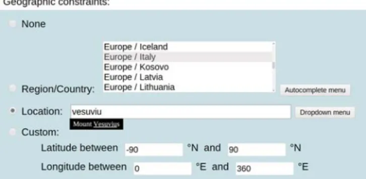
Two methods of text entry are possible for ‘Coun-try/Region’ and ‘Location’: ‘Autocomplete menu’ or ‘Dropdown menu’ (Fig. S3). The two types of entry can be changed be clicking the button to the right of the text entry ﬁeld. The default option when the query form loads is the autocomplete menu. The autocomplete menu allows the user to manually type an entry or part of an entry into the text box. When text is entered an array containing all matches is progressively displayed on the screen as a list. The list is truncated to the ﬁrst four entries in alphabeti-cal order. More entries can be revealed by clicking

Figure S3: Options in the ‘Geographic constraints’ panel, including examples of autocomplete and drop-down menus.

the down arrow below the fourth entry. Multiple countries/regions or locations can be entered by sep-arating them with commas. Alternatively, selecting the ‘Dropdown menu’ will list all locations. For ‘Country/Region’ the list is organized alphabetically by continent/ocean, followed by the country/region name, again ordered alphabetically. For ‘Location’ the location names are ordered alphabetically. The user can scroll through all entries using the right-hand scroll bar or can enter a letter of the alphabet to jump to the ﬁrst entry starting with this letter. Multiple entries can be highlighted. Model output will not be generated for multiple entries.

1.1.5 Calculate the model curves

Two sets of radio buttons are available to modify the input used to calculate location dependent curves from the five available Holocene geomagnetic field models (section 2). The left hand set allows the user to select the input coordinates. By clicking on ‘Location specified above’, the latitude and longitude of the ‘Location’ or ‘Custom’ selected in the geo-graphic constraints panel (section1.1.4) will be used to generate the model output. Model output will be produced for the geographic center of the selected location. Alternatively a different set of coordinates can be entered by clicking the radio button beneath ‘Or enter coordinates of your choice’ and entering the desired latitude and longitude into the two available text boxes. This will only change the model curve retrieved and it will plot alongside the data queried using the selection in ‘Geographic Constraints’. In both cases the coordinates are printed in .TXT file available to download.

The right hand set of radio buttons allows the user to output certain components of the spherical harmonic expansion used to construct the geomag-netic ﬁeld models. The default is to use all Gauss

(7)

coefficients up to degree 10 (the maximum degree and order of the spherical harmonic expansion for all models). Alternatively only the geocentric axial dipole (GAD) component of the field (g0₁) or the combined field from the three dipole components (GAD - g₁0 and equatorial dipoles - g1₁ and h1₁) can be calculated.

1.1.6 Abridged or detailed output

The ‘Query results’ table under the ‘Magnetic data’ tab and associated .CSV ﬁle can be appended with additional ﬁelds by selecting the detailed checkbox in the lowermost panel of the archeomagnetic and vol-canic query form. The additional entries are marked by ∗ and described in Table S1. In comparison to versions 1 and 2 of the database, site latitude and longitude are now shown by default; however, site and location names are not shown by default in the results table. These can be added by selecting the ‘Detailed’ checkbox. ‘Abridged or detailed output’

replaces the series of checkboxes previously under the panel ‘Include the following columns in results’ in versions 1 and 2 of the database (K08).

1.2 Executing a query and archeomagnetic and volcanic result tabs

To execute a query a user must click the ‘Perform Query’ button at the bottom of the query form (Fig.S1). On executing the query a new tab within the web browser will open and four “on-page” tabs will be visible (Fig. S4): (1) ‘Magnetic data’; (2) ‘Radiocarbon age data’; (3) ‘Figures and Downloads’; and (4) ‘Google Visualization’. The content of each tab is revealed by clicking on the title of the tab.

The magnetic data and radiocarbon ages results tabs are described in full in section ‘Results tables’ of B15a.

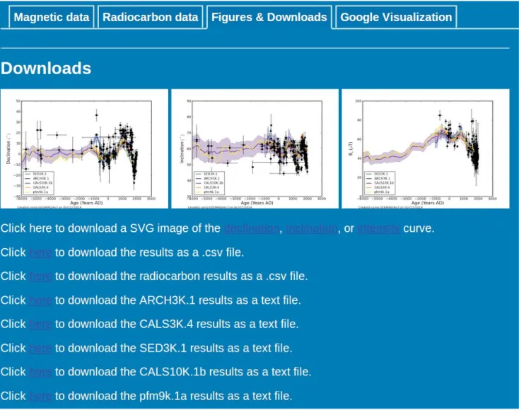
The ‘Downloads and Figures’ tab (Fig.S5) displays up to three figures (declination, inclination/ΔI and intensity/VADM with time), including model curves if selected on the query form. All figures can be downloaded as .SVG files via links below the figures or as .PNG files by saving the images themselves. The magnetic results table and radiocarbon data table can be downloaded via links to .CSV files. The format of these tables mimic the ‘Query results’ table on the ‘Magnetic data’ tab and the results table on the ‘Radiocarbon data’ tab. The only exception is that null values are replaced by -1 (for unmeasured IDs), 0 (for unspecified IDs), -999 (for null directions) or -9999 (for null ages). If model data was selected to

download on the query form, then links to .TXT ﬁles containing the model output are also displayed. The columns within these ﬁles are described in TableS3.

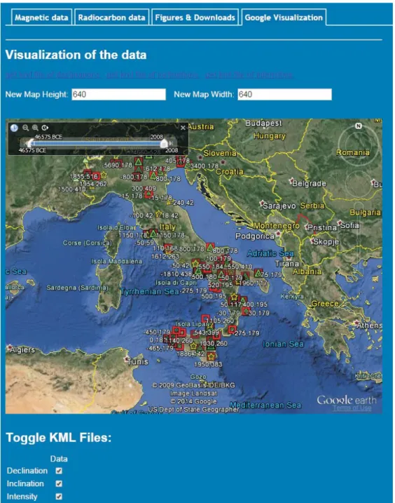
If the ‘Google Earth’ checkbox is selected on the archeomagnetic and volcanic query form (Fig.S1) a Google Earth plug-in will be launched on the ‘Google Visualization’ tab (Fig.S6). The map shown bounds all sites from countries/regions or locations selected to query. Visualization works for more than one location and with custom latitudes and longitudes. If ‘Location’ is selected in ‘Geographic Constraints’, additional locations can be entered by separating them with a comma. The map initially shows no site markers when the web page loads. Below the map are three checkboxes under ‘Toggle KML Files’. These can be selected to show sites with inclination, declination and paleointensity data.

At the top of the map is a sliding time bar, which allows sites covering diﬀerent time periods to be shown. The slide bar consists of start and end point markers that can be moved to adjust the time period. (The markers may be set to the same year when the

page initially loads and therefore no data are shown; part the markers and data will appear.) Time is given as years AD or BC.

Site declination data are shown as green triangles, inclination data are red squares and paleointensity data are gold stars. The age and reference ID are shown next to the marker, separated by a comma. A separate maker is given for declination, inclination and paleointensity obtained from the site. Clicking on one of the markers reveals a text box listing infor-mation about the site, including name, age, latitude and longitude, reference ID, and the value of the paleomagnetic measurement. Links to the .kml ﬁles that Google Earth loads to generate the visualization can be downloaded using links above the map.

The functionality of the plug-in depends on the operating system and the browser used. The plug-in works with Wplug-indows and Macplug-intosh, but is not available for Linux.

1.3 Navigation menu options

This section describes the web pages available via links on the left hand navigation bar of the main web page (http://geomagia.gfz-potsdam. de/) that are general to the whole database or spe-ciﬁc to the archeomagnetic and volcanic database. Links speciﬁc to the sediment database are described inBrown et al. (2015b).

The ‘Glossary of IDs’ web page (http: //geomagia.gfz-potsdam.de/ID_glossary.php)

(8)

Figure S4: An example of the ‘Summary of query parameters’ table and abridged ‘Query results’ table on the ‘Magnetic data’ tab. Geographic constraints: ‘Region/Country’ = Italy. Age Constraints: ‘Age between’

(9)

Figure S5: The appearance of the ‘Downloads and Figures’ tab resulting from a query of all Italian data covering the past 8 ka with all models requested to plot and download.

(10)

Figure S6: Example of a ‘Google Visualization’ for Italy. The sliding time bar has been set to the full 50 ka period and declination (green triangles), inclination (red squares) and paleointensity (gold stars) sites are all shown.

(11)

lists all metadata tables and the IDs found in the ‘Query results’ table on the ‘Magnetic data’ tab (section 1.2) and in the .CSV output ﬁle. The metadata tables shown on this page are used by both the archeomagnetic and volcanic database and the sediment database (Brown et al., 2015b). The metadata table names are listed at the top of the page. Each table is a hyperlink and clicking on the metadata table name takes the user to the appropriate metadata table. The web page automatically updates as new entries are added to the metadata tables.

The ‘Available archeomagnetic and volcanic stud-ies’ web page (http://geomagia.gfz-potsdam.de/ studies.php) contains a full reference list for studies included in the database. The number of references currently within the database is listed above the ref-erence table header. The refref-erences can be ordered by ID, first author surname, year of publication and journal. The IDs are the same as those listed un-der ‘Reference ID’ in the ‘Query results’ table on the ‘Magnetic data’ tab (section 1.2) and the .CSV output file. The final column lists hyperlinks to the MagIC database (http://earthref.org/MAGIC/), if data from a particular reference are also stored within the MagIC database. Two search boxes allow the user to search for references based on author or by words contained within the title of a publication. The author search will search through all authors and coauthors.

The ‘Statistics’ web page (http://geomagia. gfz-potsdam.de/statistics.php) tracks the num-ber of queries executed and plots the past 30 days’ activity. The ‘Credits’ web page (http://geomagia. gfz-potsdam.de/credits.php) lists contributors to GEOMAGIA50 across all incarnations. The ‘Logs’ web page (http://geomagia.gfz-potsdam.

de/logs.php) tracks any signiﬁcant changes made to the database, such as if an error was corrected in a data set, if new data are added, or if a modiﬁca-tion to the interface or a structural change to the database was made.

2 Global models of the Holocene

geomagnetic ﬁeld

Location dependent predictions of inclination, dec-lination and intensity can currently be generated from ﬁve temporally continuous global models of the Holocene geomagnetic ﬁeld: CALS3k.4, CALS10k.1b, ARCH3k.1, SED3k.1 and pfm9k.1a. The models are determined by a regularized least squares inversion

of archeo- and paleomagnetic data using spherical harmonics in space and cubic B-splines in time. With the exception of pfm9k.1a, models produce bootstrap estimates of uncertainty for their magnetic compo-nents. CALS3k.4 and CALS10k.1b are constrained to agree closely to gufm1 (Jackson et al.,2000) for the past four centuries, whereas ARCH3k.1 and SED3k.1 are only loosely constrained and pfm9k.1a is not con-strained by gufm1. Caution must be used when gener-ating model output from regions sparse in data. They may have uncertainties larger than the estimates de-termined by the bootstrap calculations. Work on calculating global models of the geomagnetic ﬁeld is ongoing and new models may be added to the search interface as they become available.

CALS3k.4 (Korte and Constable, 2011) uses a combination of archeomagnetic and sediment data covering the past 3 ka available up to 2011. It super-seded CALS3k.3 (Donadini et al., 2009; Korte et al.,

2009) and incorporated 163 additional archeomag-netic data and 13 newly published sediment records in its construction. This resulted in notable diﬀer-ences between the two models over South-East Asia, Alaska and Siberia. Although bootstrap estimates of uncertainty are provided, the prediction is the best ﬁt model, not CALS3k.4b (which is an average from bootstrap sampling as used in the creation of CALS10k.1b).

CALS10k.1b (Korte et al.,2011) covers the past 10 ka and incorporates the largest number of data to date. CALS10k.1b supersedes CALS7K.2 (Korte et al., 2005; Korte and Constable, 2005). It is based on sediment, lava and archeological data available up to 2011. The data compilation is dominated by sediment data as archeomagnetic and lava data are sparse prior to 1000 BC. The ﬁnal model is an aver-age obtained from bootstrap sampling (the ‘b’ in the model name denoting bootstrap sampling) to account for uncertainties in paleomagnetic and chronological data. Consequently, it is smoothed strongly com-pared with CALS3k.4. This allowed reconstruction of earlier epochs, where data are sparser.

ARCH3k.1 (Korte et al.,2009) was constructed us-ing available archeomagnetic data up to 2009. It cov-ers the past 3 ka. Data are strongly biased towards the Northern Hemisphere and Europe in particular. The model gives reasonable ﬁeld values for the North-ern Hemisphere, but should not be used for global studies or Southern Hemisphere ﬁeld predictions.

SED3k.1 (Korte et al.,2009) was constructed us-ing available sediment data up to 2009 and covers the past 3 ka. Data have a better global distribu-tion (less biased towards the Northern Hemisphere)

(12)

than ARCH3k.1 and can be used for predictions in the Southern Hemisphere. The model output is smoothed in time as a result of the sedimentary recording process and the methods of sub-sampling employed.

The pfm9k.1a model (Nilsson et al.,2014), spans the past 9000 years. It uses the same data set as CALS10k.1b, but employs new data treatments, par-ticularly for sedimentary data. These include redis-tributing the weight given to diﬀerent data types and data sources, iteratively recalibrating relative declination data and adjusting the timescales of the sediment records using a preliminary model. These data treatments, particularly the timescale adjust-ments, reduce inconsistencies in the data set and enable pfm9k.1a to capture larger amplitude pale-osecular variations. The model is valid up to 1900 AD.

Users should note that when comparing site data with model predications generated for locations span-ning large geographic areas, the diﬀerence between the site latitude and longitude and the coordinates used to generate the model predictions can vary by tens of degrees. Model predictions are generated for the geographic centers of the areas in question. A site’s coordinates can therefore be far from those used in the model query. This can result in oﬀsets between the data and the model predictions. This is purely from the geographic constraint selected and is not a limitation of the models.

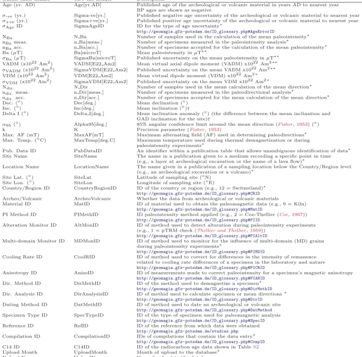
3 Description of database output

This section contains 3 tables. Table S1 and S2 describe the output headers of the online results tables and the .CSV data files for the archeomagnetic query. TableS3describes the column headers for the .TXT files containing the output from models of the Holocene geomagnetic field (section 2).

References

Brown, M. C., F. Donadini, M. Korte, A. Nilsson, K. Korhonen, A. Lodge, S. N. Lengyel, and C. G. Constable (2015a), GEOMAGIA50.v3: 1. general structure and modiﬁcations to the archeological and volcanic database, Earth Planets Space, doi: 10.1186/s40623-015-0232-0.

Brown, M. C., F. Donadini, U. Frank, S. Panovska, A. Nilsson, K. Korhonen, M. Schuberth, M. Korte, and C. G. Constable (2015b), GEOMAGIA50.v3:

2. a new paleomagnetic database for lake and ma-rine sediments, Earth Planets Space, 67, 70, doi: 10.1186/s40623-015-0233-z.

Coe, R. S. (1967), Paleo-intensities of the Earth’s magnetic ﬁeld determined from Tertiary and Qua-ternary rocks, J. Geophys. Res., 72, 3247–3262, doi:10.1029/JZ072i012p03247.

Donadini, F., M. Korte, and C. Constable (2009), Geomagnetic ﬁeld for 0-3 ka: 1. New data sets for global modeling, Geochem. Geophys. Geosyst., 10, Q06,007, doi:10.1029/2008GC002295.

Fisher, R. A. (1953), Dispersion on a sphere, Proc.

R. Soc. Lond., A, 217, 295–305, doi:10.1098/rspa.

1953.0064.

Jackson, A., A. R. T. Jonkers, and M. R. Walker (2000), Four centuries of geomagnetic secular vari-ation from historical records, Phil. Trans. R. Soc.

Lond. A, 358, 957–990, doi:10.1098/rsta.2000.0569.

Korte, M., and C. Constable (2011), Improving ge-omagnetic ﬁeld reconstructions for 0-3 ka, Phys.

Earth Planet. Inter., 188, 247–259, doi:10.1016/j.

pepi.2011.06.017.

Korte, M., and C. G. Constable (2005), Continuous geomagnetic ﬁeld models for the past 7 millenia: 2. CALS7K, Geochem. Geophys. Geosyst., 6, Q02H16, doi:10.1029/2004GC000801.

Korte, M., A. Genevey, C. G. Constable, U. Frank, and E. Schnepp (2005), Continuous geomagnetic ﬁeld models for the past 7 millenia: 1. a new global data compliation, Geochem. Geophys. Geosyst., 6, Q02H15, doi:10.1029/2004GC000800.

Korte, M., F. Donadini, and C. G. Constable (2009), Geomagnetic ﬁeld for 0-3 ka: 2. a new series of time-varying global models, Geochem. Geophys.

Geosyst., 10, Q06,008, doi:10.1029/2008GC002297.

Korte, M., C. Constable, F. Donadini, and R. Holme (2011), Reconstructing the Holocene geomagnetic ﬁeld, Earth Planet. Sci. Lett., 312, 497–505, doi: 10.1016/j.epsl.2011.10.031.

Nilsson, A., R. Holme, M. Korte, N. Suttie, and M. Hill (2014), Reconstructing Holocene geomag-netic ﬁeld variation: new methods, models and implications, Geophys. J. Int., 198, 229–248, doi: 10.1093/gji/ggu120.

(13)

Shaw, J. (1974), A new method of determining the magnitude of the palaeomagnetic field. Applica-tion to five historic lavas and five archaeological samples, Geophys. J. R. astr. Soc., 39, 133–141, doi:10.1111/j.1365-246X.1974.tb05443.x.

Thellier, E., and O. Thellier (1959), Sur l’intensité du champ magnétique terrestre dans le passé his-torique et géologique, Ann. Géophys., 15, 285–376.

(14)

Online table header CSV ﬁle header Description

Age (yr. AD) Age[yr.AD] Published age of the archeological or volcanic material in years AD to nearest year BP ages are shown as negative

σ-ve(yr.) Sigma-ve[yr.] Published negative age uncertainty of the archeological or volcanic material to nearest year

σ+ve(yr.) Sigma+ve[yr.] Published positive age uncertainty of the archeological or volcanic material to nearest year

σAgeID SigmaAgeID ID for the type of age uncertainty∗

http://geomagia.gfz-potsdam.de/ID_glossary.php#AgeErrorID

NBa N Ba Number of samples used in the calculation of the mean paleointensity∗

nBameas. n Ba[meas.] Number of specimens measured in the paleointensity analysis∗

nBaacc. n Ba[acc.] Number of specimens accepted for the calculation of the mean paleointensity∗

Ba (μT) Ba[microT] Mean paleointensity inμT∗∗

σBa(μT) SigmaBa[microT] Published uncertainty on the mean paleointensity inμT∗∗

VADM (x1022Am2) VADM[E22 Am2] Mean virtual axial dipole moment (VADM) x1022Am2∗∗

σVADM(x1022Am2) SigmaVDM[E22 Am2] Published uncertainty on the mean VADM x1022Am2∗∗

VDM (x1022Am2) VDM[E22 Am2] Mean virtual dipole moment (VDM) x1022Am2∗

σVDM(x1022Am2) SigmaVDM[E22 Am2] Published uncertainty on the mean VDM x1022Am2∗

Ndir. N Dir Number of samples used in the mean calculation of the mean direction∗

ndir.meas. n Dir[meas.] Number of specimens measured in the paleodirectional analysis∗

ndir.acc. n Dir[acc.] Number of specimens accepted for the mean calculation of the mean direction∗

Dec. (◦) Dec[deg.] Mean declination (◦) Inc. (◦) Inc[deg.] Mean inclination (◦)†

Delta I (◦) Delta I[deg.] Mean inclination anomaly (◦) (the diﬀerence between the mean inclination and GAD inclination for the site)†

α95(◦) Alpha95[deg.] 95% angular conﬁdence limit around the mean direction (Fisher,1953) (◦)

k K Precision parameter (Fisher,1953)

Max. AF (mT) MaxAF[mT] Maximum alternating ﬁeld (AF) used in determining paleodirections∗ Max. Temp. (◦C) MaxTemp[deg.C] Maximum temperature used during thermal demagnetization or during

paleointensity experiments∗

Pub. Data ID PubDataID An identifier within a publication table that allows unambiguous identification of data∗ Site Name SiteName The name in a publication given to a medium recording a specific point in time

(e.g., a layer at archeological excavation or the name of a lava ﬂow)∗

Location Name LocationName The name given in a publication of a sampling location below the Country/Region level (e.g., an archeological excavation or a volcano)∗

Site Lat. (◦) SiteLat Latitude of sampling site (◦N) Site Lon. (◦) SiteLon Longitude of sampling site (◦E)

Country/Region ID CountryRegionID ID of the country or region (e.g., 12 = Switzerland)∗ http://geomagia.gfz-potsdam.de/ID_glossary.php#CRID Archeo/Volcanic ArcheoVolcanic Whether the data from archeological or volcanic materials

Material ID MatID ID of material used to obtain the paleomagnetic data (e.g., 9 = Kiln) http://geomagia.gfz-potsdam.de/ID_glossary.php#MatID

PI Method ID PIMethID ID paleointensity method applied (e.g., 2 = Coe-Thellier (Coe,1967)) http://geomagia.gfz-potsdam.de/ID_glossary.php#PIID

Alteration Monitor ID AltMonID ID of method used to detect alteration during paleointensity experiments (e.g., 1 = pTRM check (Thellier and Thellier,1959))

http://geomagia.gfz-potsdam.de/ID_glossary.php#PIAltID

Multi-domain Monitor ID MDMonID ID of method used to monitor for the inﬂuence of multi-domain (MD) grains during paleointensity experiments∗

http://geomagia.gfz-potsdam.de/ID_glossary.php#PIMDID

Cooling Rate ID CoolRID ID of method used to correct for diﬀerences in the intensity of remanence related to cooling rate diﬀerences of a specimen in the laboratory and nature http://geomagia.gfz-potsdam.de/ID_glossary.php#PICRID

Anisotropy ID AnisoID ID of measurements made to correct paleointensity for a specimen’s magnetic anisotropy http://geomagia.gfz-potsdam.de/ID_glossary.php#PIANID

Dir. Method ID DirMethID ID of the method used to demagnetize a specimen∗ http://geomagia.gfz-potsdam.de/ID_glossary.php#DirMethID Dir. Analysis ID DirAnalysisID ID of methid used to calculate specimen or mean directions∗

http://geomagia.gfz-potsdam.de/ID_glossary.php#DirID Dating Method ID DatMethID ID of method used to date an archeological or volcanic site

http://geomagia.gfz-potsdam.de/ID_glossary.php#DatMethod Specimen Type ID SpecTypeID ID of the type of specimen used for paleomagnetic analysis

http://geomagia.gfz-potsdam.de/ID_glossary.php#SpecID Reference ID RefID ID of the reference from which data were obtained

http://geomagia.gfz-potsdam.de/studies.php Compilation ID CompilationID IDs of compilations that contain the data entry∗

http://geomagia.gfz-potsdam.de/ID_glossary.php#CompID C14 ID C14ID ID of the radiocarbon age data shown in TableS2 Upload Month UploadMonth Month of upload to the database∗

Upload Year UploadYear Year of upload to the database

UID UID Unique identiﬁcation number for the entry

Table S1: Column headers for online and .CSV magnetic data results table. Fields are arranged in order of appearance in table. IDs are numbers in corresponding relational tables. These are given below the online metadata relational tables and linked via hyperlinks from the ID. ∗The ‘Detailed’ check box at the bottom of the archeomagnetic and volcanic query form (Fig.S1) must be activated to include these columns in the output;∗∗output will either be Ba and σBa or VADM and σVADM depending on which checkbox is activated

under ‘Select data types to output’ in the ‘Query, Plot, Visualize’ box at the top of the archeomagnetic and volcanic query form (Fig.S1); †output will either be inclination or inclination anomaly depending on which checkbox is activated under ‘Select data types to output’ in the ‘Query, Plot, Visualize’ box at the top of the archeomagnetic and volcanic query form (I or delta I).

(15)

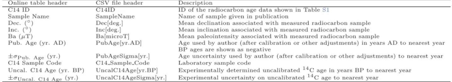
Online table header CSV ﬁle header Description

C14 ID C14ID ID of the radiocarbon age data shown in TableS1 Sample Name SampleName Name of sample given in publication

Dec. (◦) Dec[deg.] Mean declination associated with measured radiocarbon sample Inc. (◦) Inc[deg.] Mean inclination associated with measured radiocarbon sample Ba (μT) Ba[microT] Mean paleointensity associated with measured radiocarbon sample

Pub. Age (yr. AD) PubAge[yr.AD] Age used by author (after calibration or other adjustments) in years AD to nearest year BP ages are shown as negative

±σPub. Age(yr.) PubAgeSigma[yr.] Age uncertainty used by author (after calibration or other adjustments) to nearest year

C14 Sample Code C14 Sample Code Laboratory sample code

Uncal. C14 Age (yr. BP) UncalC14Age[yr.BP] Experimentally determined uncalibrated14C age in years BP to nearest year

±σUncal. C14 Age(yr.) UncalC14AgeSigma[yr.] Experimental uncertainty on uncalibrated14C age to nearest year

Table S2: Column headers for the online and .CSV radiocarbon age tables results table. Fields are arranged in order of appearance in table. IDs are numbers in corresponding relational tables. These are given below the online tables and linked via hyperlinks from the ID.

Model output column Description

AGE BP Time in years BP (1950 AD is 0 years BP)

AGE AD Time in years AD/BC (where is AD is positive and BC is negative)

SITE LAT Latitude (◦N) of the Country/State/Region/Sea; Location; or Core selected to query SITE LON Longitude (◦E) of the Country/State/Region/Sea; Location; or Core selected to query INCL Inclination (◦)

DELTAI Inclination anomaly (◦) DECL Declination (◦) INT Paleointensity (μT)

VADM Virtual Axial Dipole Moment (E1022Am22) EI Bootstrap uncertainty estimates of inclination (◦) ED Bootstrap uncertainty estimates of declination (◦) EF Bootstrap uncertainty estimates of intensity (μT)

EM Bootstrap uncertainty estimates of Virtual Axial Dipole Moment (x1022Am22)

Table S3: Description of CALSxk and pfm9k.1a model output columns. If ‘Country/State/Region/Sea’ is selected on the query form, the latitude and longitude of the geographical center of that area will be listed.