Interferometric measurements beyond the coherence length of the laser source

Interferometric measurements beyond the

coherence length of the laser source

Y

S

,

F

P

,

M

R

,

A

P

,

Y

M

,

S

M

,

O

G

,

M

L

,

R

M

,

J

F

,

F

G

,

G

M

1_{Haute Ecole ARC Ingénierie (University of Applied Sciences of Western Switzerland), Rue de la Serre} 7, 2610 Saint-Imier, Switzerland

2_{Hexagon Technology Center GmbH, Heinrich-Wild-Strasse, 9435 Heerbrugg, Switzerland}

3_{Laboratory Time and Frequency, University of Neuchâtel, Avenue de Bellevaux 51, 2009 Neuchâtel,} Switzerland

*yves.salvade@he-arc.ch

Abstract: Interferometric measurements beyond the coherence length of the laser are

investigated theoretically and experimentally in this paper. Thanks to a high-bandwidth detection, high-speed digitizers and a fast digital signal processing, we have demonstrated that the limit of the coherence length can be overcome. Theoretically, the maximal measurable displacement is infinite provided that the sampling rate is sufficiently short to prevent any phase unwrapping error. We could verify experimentally this concept using a miniature interferometer prototype, based on a frequency stabilized vertical cavity surface emitting laser. Displacement measurements at optical path differences up to 36 m could be realized with a relative stability better than 0.1 ppm, although the coherence length estimated from the linewidth and frequency noise measurements do not exceed 6.6 m.

OCIS codes: (030.0030) Coherence and statistical optics; (120.3180) Interferometry; (120.5050) Phase measurement.

References and links

1. Y. Kotaki and H. Ishikawa, “Wavelength tunable DFB and DBR lasers for coherent optical fibre communications,” IEE Proc., J Optoelectron. 138(2), 171–177 (1991).

2. R. Michalzik, VCSELs: Fundamentals, Technology and Applications of Vertical-Cavity Surface-Emitting Lasers (Springer, 2012)

3. U. Hofbauer, E. Dalhoff, and H. Tiziani, “Double-heterodyne-interferometry with delay-lines larger than coherence length of the laser light used,” Opt. Commun. 162(1-3), 112–120 (1999).

4. E. Fischer, E. Dalhoff, and H. Tiziani, “Overcoming coherence length limitation in two wavelength interferometry - an experimental verification,” Opt. Commun. 123(4–6), 465–472 (1996).

5. M. Rohner and T. Jensen, “Phase noise compensation for interferometric absolute rangefinders,” US patent no US7619719 B2, 2009.

6. X. Fan, Y. Koshikiya, and F. Ito, “Phase-noise-compensated optical frequency domain reflectometry with measurement range beyond laser coherence length realized using concatenative reference method,” Opt. Lett. 32(22), 3227–3229 (2007).

7. Z. Ding, X. S. Yao, T. Liu, Y. Du, K. Liu, Q. Han, Z. Meng, J. Jiang, and H. Chen Ding, “Long Measurement Range OFDR Beyond Laser Coherence Length,” IEEE Photonics Technol. Lett. 25(2), 202–205 (2013). 8. A. Papoulis, Probability, Random Variables, and Stochastic Processes (McGraw-Hill, 1984)

9. L. Mandel and E. Wolf, “Coherence Properties of Optical Fields,” Rev. Mod. Phys. 37(2), 231–287 (1965). 10. J. W. Goodman, Statistical Optics (Wiley, 1985), Chap. 5.

11. K. Petermann, Laser Diode Modulation and Noise (Kluwer Academic, 1988), Chap. 7.

12. Y. Salvadé and R. Dändliker, “Limitations of interferometry due to the flicker noise of laser diodes,” J. Opt. Soc. Am. A 17(5), 927–932 (2000).

13. Y. Petremand, C. Affolderbach, R. Straessle, M. Pellaton, D. Briand, G. Mileti, and N. F. de Rooij, “Microfabricated rubidium vapour cell with a thick glass core for small-scale atomic clock applications,” J. Micromech. Microeng. 22(2), 025013 (2012).

14. J. Di Francesco, F. Gruet, C. Schori, C. Affolderbach, R. Matthey, G. Mileti, Y. Salvadé, Y. Petremand, and N. De Rooij, “Evaluation of the frequency stability of a VCSEL locked to a micro-fabricated Rubidium vapour cell,” Proc. SPIE 7720, 77201T (2010).

15. J. Wu, Z. Yaqoob, X. Heng, X. Cui, and C. Yang, “Harmonically matched grating-based full-field quantitative high-resolution phase microscope for observing dynamics of transparent biological samples,” Opt. Express 15(26), 18141–18155 (2007).

16. Virtex-6 FPGA SelectIO Resources - User guide (Xilinx doc no UG361 (v1.6), 2014), Chap. 3, http://www.xilinx.com/support/documentation/user_guides/ug361.pdf

17. F. Gruet, A. Al-Samaneh, E. Kroemer, L. Bimboes, D. Miletic, C. Affolderbach, D. Wahl, R. Boudot, G. Mileti, and R. Michalzik, “Metrological characterization of custom-designed 894.6 nm VCSELs for miniature atomic clocks,” Opt. Express 21(5), 5781–5792 (2013).

18. Hexagon Metrology white paper, “Leica absolute interferometer - A New Approach to Laser Tracker Absolute Distance Meters” (Hexagon Metrology, 2012).

http://metrology.leica- geosystems.com/downloads123/m1/metrology/general/white-tech-paper/Leica%20Absolute%20Interferometer_white%20paper_en.pdf 1. Introduction

Nowadays, laser diodes are inexpensive coherent sources which are integrated in several consumer products (optical disk drive, optical mice, laser pointers, laser printers, barcode readers, etc.). However, most commercially available interferometric devices (machine tool calibrators, vibrometer, etc.) are still based on Helium Neon (He-Ne) lasers, mainly because of their high temporal and spatial coherences. Although Fabry-Perot laser diodes are very commonly used and inexpensive, they are affected by frequency mode hops, preventing their application in wavelength standards for high-accuracy displacement measurements. Usage of a Bragg grating, acting as a frequency selective mirror, allows to increase drastically the mode-hop-free tuning range. Distributed Bragg reflector and feedback lasers contain a grating region and exhibit narrow linewidth (typ. a few MHz or less) and stable single-frequency operation [1]. However their cost is high. Vertical-cavity surface-emitting lasers (VCSEL) are manufactured in mass quantity (mainly for the computer mice market) and are now commercially available from many suppliers at very cheap prices. They are composed of at least one Bragg grating and demonstrate circular output beam shape [2]. However, their spectral linewidth of about 25-100 MHz, depending on the devices, is much wider compared to that of He-Ne lasers (usually smaller than 1 MHz), thus making long displacement measurements difficult.

The maximal optical path difference that can be measured using an interferometer is commonly estimated by the well-known coherence length of the laser, inversely proportional to the spectral linewidth. At the limit of the coherence length, the interference fringe visibility is reduced for low detection bandwidths, and the interferometric phase noise becomes much higher. It is however important to mention that the coherence length is not a strict limit on the maximal distance or displacement that can be measured in an interferometric way. The reduction of fringe visibility can be easily overcome by using high-detection bandwidths, but the interference signal is then strongly affected by phase noise. Nevertheless, measurements beyond the coherence length have been reported for absolute distance measurements: Hofbauer [3] and Fisher [4] achieved absolute distance measurements beyond the coherence length of the laser using a superheterodyne two-wavelength interferometer, where the frequency difference between the two sources is generated by an acousto-optic modulator working at 500 MHz. The common-mode frequency noise of the two wavelengths was suppressed by detecting directly the interferometric phase difference at both wavelengths. Several solutions based on reference interferometers were also proposed in scientific and patent literature, in order to compensate the interferometric phase noise for absolute range finders [5] or for optical frequency domain reflectometry [6,7].

In this paper, we propose a novel type of miniature interferometer for displacement measurements over long ranges based on a low-cost laser source with a moderate coherence length. Measurement beyond the coherence length is enabled thanks to a high-speed digital signal processing implemented in an embedded electronic system. In addition, innovative

concepts have been applied to reach a miniature and potentially cost effective optical set-up, while keeping sub-ppm resolution.

In the following section, we will at first briefly remind the basics of temporal coherence, and present measurements of frequency noise of VCSELs, from which coherence length and linewidths are calculated. Then, in section 3, the statistics of the detected interferometric signal phase will be investigated; we will also discuss the limits on the maximal measurable range, in case of a classical single-wavelength incremental interferometer. We will see that displacement measurements over infinite distances are theoretically feasible, using an appropriate detection bandwidth and a sufficiently fast sampling rate. The experimental verification of the concept is presented in section 4. A miniature interferometer based on a frequency stabilized VCSEL will be presented, as well as interferometric measurements beyond the coherence length.

2. Temporal coherence and laser frequency noise

2.1 Basics

It is well-known that the spectral linewidth of a laser is caused by its phase (or frequency) noise. Indeed, for quasi-monochromatic light, the complex wave function is of the form

[

]

(

)

( ) exp ( ) exp 2

V t =V i tφ i πνt (1)

where ν = c/λ is the optical frequency of the laser light, and φ(t) represents the random fluctuations of the phase. In an interferometer, the two interfering beams travel over different optical paths, and are therefore delayed from each other by τ = OPD/c, where OPD is the optical path difference and c is the light speed. In a Michelson interferometer, OPD is equal to 2nD, where n is the index of refraction of air (n ≈1) and D is the length difference of the interferometer arms. The time-averaged interference signal is therefore given by

(

)

[

]

{

}

where φi(τ,t) = φ(t) − φ(t − τ) is the instantaneous phase noise of the interference signal. The

function C(τ) describes the envelope of the interference signal, and can also be interpreted as the fringe visibility. It can easily be demonstrated that the fringe visibility is also given by the magnitude of the normalized autocorrelation function g(τ) of the complex field V(t)

[

]

The instantaneous phase noise is caused by a large number of independent contributions. According to the central limit theorem [8], we can consider in a good approximation that it follows a Gaussian probability density function. Therefore, the ensemble average in Eq. (3) can be calculated, and we find

2 1 ( ) ( ) exp ( , ) . 2 i Cτ = g τ = _− φ τ t _   (5)

The interferometric delay at which the fringe visibility decreases to a prescribed value (e.g. 1/e or 1/2) is known as the coherence time of the source τc. The Mandel’s definition is commonly used in statistical optics literature [9,10], i.e.

2 ( ) . c g d τ +∞ τ τ −∞ =

_

Consequently, the coherence length is given by c·τc. Coherence time and coherence length are inversely proportional to the emission linewidth Δν of the source, because the power spectrum of the source is related to g(τ) by a Fourier transform (Wiener-Kintchine theorem). The exact relation between Δν (full width at half maximum, FWHM) and τc depends on the line shape function. The spectral line shape of a single-mode laser is usually considered to be a Lorentzian function. In this particular case, the relation is τc = 1/(πΔν). However, the frequency noise of laser diodes (and especially VCSELs), exhibits a strong flicker noise [11] and unfortunately, the Lorentzian approximation is not valid any more.

The frequency fluctuations of a laser are conveniently described by a power spectral density (PSD). Contrary to He-Ne laser whose frequency noise PSD is mainly composed of a white-noise part, the PSD of the frequency fluctuations of laser diodes is of the form

0 1

( )_{free running} / .

S∂_ν f =C +C fα (7)

As interferometers measure displacements in terms of laser wavelength, the measurement accuracy over long distances is limited by the wavelength accuracy and stability. It is therefore mandatory to stabilize the optical frequency with respect to an absolute frequency standard (for instance, rubidium or cesium absorption cells). The frequency fluctuations are thus reduced at low frequencies, thanks to the stabilization loop. It can be shown that the frequency stabilization that uses an integral feedback shapes the power spectral density of the frequency noise according to

(

)

where fc is the cut-off frequency of the integrator regulator. The PSD of the instantaneous phase noise in an interferometer is related to the Sδν(f) by the relation [12]

(

)

We note that the interferometer acts as a low-pass filter with a bandwidth of 1/τ. Its transfer function (sinc function) corresponds actually to a moving average process over the time window τ. The variance <φi(τ,t)2> can then be calculated using the Parseval relation

2 0

( , t) _i( , ) .

i Sφ f df

φ τ =∞

_

Using Eqs. (5)-(10), we see that |g(τ)| and thus the coherence time can be derived from the frequency noise of the laser source. In addition, we can also calculate the spectral line shape from a Fourier transform of |g(τ)|, and thus find the linewidth of the laser. The knowledge of Sδν(f) is thus of a great importance to determine the temporal coherence of a laser diode. 2.2 Frequency noise measurements of laser diodes

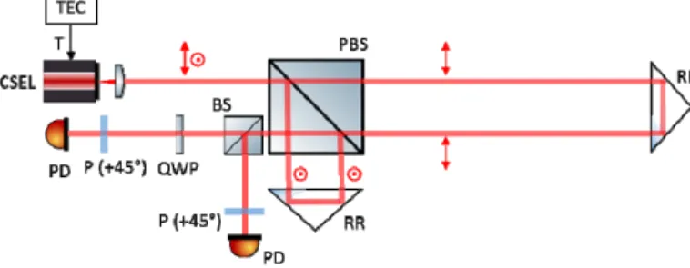
We measured the frequency noise of two 780 nm VCSELs from the company ULM Photonics (ULM780-01-TN). The two lasers came from two difference batches (One of the VCSEL was manufactured in 2009, and the other one in 2011). We measured actually the instantaneous phase noise in a Michelson-type interferometer with an arm length difference D of about 1.15m, corresponding to an OPD of 2.3 m. The interferometer, as depicted in Fig. 1, enables quadrature detection by means of polarization: The incoming light enters a polarizing

beamsplitter with a linear polarization oriented at 45° with respect to the horizontal/vertical axes. The horizontal component of the incoming polarization is transmitted over the long arm, as the vertical component is reflected towards the reference arm. After the reflections on the two retroreflectors, the two polarizations are recombined. The outgoing beam is then splitted in two channels, and directed towards two photodetectors behind linear polarizers oriented at 45°. In one of the channels, a quarter waveplate is located just before the polarizer to introduce a phase shift of 90° between the two orthogonal polarizations

Fig. 1. Optical set-up for frequency noise measurement. TEC: thermo-electric temperature control, PBS: polarizing beamsplitter, RR: retroreflector, BS: beamsplitter (non-polarizing), QWP: quarter waveplate, P: linear polarizer, PD: photodector.

Since the detection bandwidth of the detectors (about 150 MHz) is higher than the interferometer bandwidth 1/τ, the filtering process caused by the photodetectors can be neglected. The offsets and amplitude of the two interference signals were first calibrated, by modulating the current (and thus the frequency) of the VCSEL. After offset subtraction, and normalization of the amplitude of the interference terms, we got finally

[

]

[

]

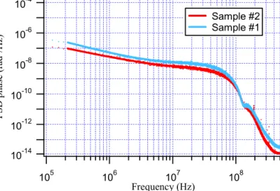
The instantaneous phase fluctuations were calculated using the function atan2(S1,S2). The phase was then unwrapped, and the power spectral density of the phase noise was retrieved. To ensure that the phase was not affected by 2π phase jumps, the interference signals had to be sampled with a sampling rate much higher than the detection bandwidth. The signals were acquired by means of a digitizing scope working at a sampling rate of 4 GS/s. As shown in Fig. 2, the measured phase noises are different for the two samples (The standard deviation of the phase noise was two times smaller for Sample #2), indicating a relatively large batch-to-batch difference in terms of frequency noise.

The parameters C0, C1 and α of the frequency noise were determined for the two VCSEL samples by fitting the measurement data with the model function described by Eq. (9), using τ = OPD/c = 7.6 ns. With Eqs. (8)-(10) we could then evaluate numerically the variance of the instantaneous phase for several delays τ, and the magnitude of the complex degree of coherence |g(τ)| using Eq. (5). The cut-off frequency fc of the stabilization loop was set to 1 kHz. A fast Fourier transform of |g(τ)| allowed us to find the spectral lineshapes of the two laser samples (they are shown in Fig. 3), from which the laser linewidths (FWHM) could be directly retrieved. Finally, the coherence time τc (and coherence length lc = c·τc) could be calculated using Eq. (6). Results are summarized in Table 1.

To confirm the process of deriving the various parameters from the instantaneous phase measurements, the linewidth of sample #2 was additionally measured by means of a Fabry-Perot interferometer. The observation of 27 MHz agrees very well with the estimated value presented in Table 1.

10-14 10-12 10-10 10-8 10-6 10-4 PS D phas e (rad 2 /H z) 105 106 107 108 Frequency (Hz) Sample #2 Sample #1

Fig. 2. Power spectral density of the phase noise measured at an interferometer arm length difference D = 1.15 m, using two VCSELs from two different batches.

1.0 0.8 0.6 0.4 0.2 0.0 Vi sib ilit y 100 80 60 40 20 0 Interferometric delay (ns) S pectru m ( a. u. ) -40 0 40 Frequency (MHz) a) b)

Fig. 3. (a) Calculated visibility, and (b) spectral lineshape for the two VCSELs. Blue curve: sample #1, red curve: sample #2.

Table 1. Summary of the frequency noise, coherence and linewidth parameters estimated for the two VCSELs

Frequency noise Coherence Linewidth

(FWHM) Sample # C0 (Hz) C1 (Hz1+α) α τc (ns) lc (m) Δν (MHz)

1 3.8·106 _7.4·1013 _{1.1 11 3.3 51}

2 1.6·106 _2.4·1012 _{0.9 5.5 6.6 26}

3. Detected phase noise

The filtering process caused by the finite detection bandwidth must be considered if B < 1/τ. The detected interference signal is therefore of the form

(

)

[

]

{

}





where h(t) is the normalized impulse response of the filter process. For low-phase noise (<< 1), we have

[

]

exp iφ τi( , )t ≈ +1 iφ τi( , ).t (13) Under this assumption, we have

[

]









Therefore, the filtering process on the interference signal can be approximated as the filter applied to the instantaneous phase noise, i.e.

1 1

( , ) ( ) ( , ) . D t h t t i t dt

φ τ =

_

Consequently, the PSD of the detected phase noise is

2

( ,f) ( ,f) ( ) ,

D i

S_φ τ =S_φ τ H f (16)

where H(f) is the frequency response of the detectors. For a first-order system of bandwidth B, we have 1 ( ) . 1 / H f if B = + (17)

Again, the variance of the detected phase is given by the Parseval relation

2 0

( , t) _D( , ) .

D Sφ f df

φ τ =∞

_

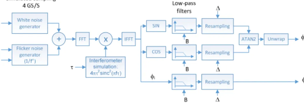
As already mentioned, Eq. (16) is realistic only for low phase noise (i.e. short distances), or when B > 1/τ (i.e. long distances), since the detection low-pass filter is then negligible compared to the moving average filter caused by the interferometer. For medium distances, Eq. (16) may yield invalid results. In order to investigate the behavior for high phase noise and detection bandwidth B < 1/τ, we proceeded to Monte-Carlo simulations. The Monte-Carlo simulation tool is described by the block diagram depicted in Fig. 4. Gaussian white noise sequences were emulated by using pseudo-random number generators. The flicker noise sequences were generated by using other Gaussian white noise sequences followed by a 1/fα filter. The noise amplitudes were adapted to get a frequency noise spectrum very close to the frequency noise measured for sample #1. We simulated then the low-pass filter caused by the interferometer (sinc function), the two interference signals in quadrature, the low-pass filter caused by the finite detection bandwidth, the sampling process (with sampling time Δ), and finally the phase detection algorithm (atan2 function followed by a phase unwrapping operation). This latter operation generated the phase noise φMC. In parallel, we calculated also the phase φD that would be obtained by directly applying the low-pass filter on the instantaneous phase noise sequences φi, as assumed in Eq. (15). The deviation between the two resulting phases is then estimated using the root-mean-square error

(

)

. D MC

RMSE= φ −φ (19)

This error, as well as the standard deviation of φMC, were estimated for different detection bandwidths and for several distances ranging from 1 cm to 150 m. Results are in shown in Fig. 5(a). For high bandwidths, the two phases φD and φMC are in good agreement (RMSE < 0.03 rad). However, the simulation results show a drastic increase of RMSE for bandwidth B < 100 MHz and distances above 1 m. It turns out that this high deviation is caused by frequent

2π phase jumps of φMC resulting from phase unwrapping errors, even for a sampling time as short as 1 ns. For bandwidths ≥ 100 MHz and Δ = 1 ns, the phase jumps totally disappear. Figure 5(b) shows the standard deviation of the detected phase as function of the interferometer arm length difference D, for bandwidths of 100 MHz and 200 MHz. The solid curves have been calculated from Eqs. (8), (9), and Eqs. (16)-(18), and the frequency noise parameters of VCSEL sample #1. The dots are the values simulated by our Monte-Carlo model. As shown in Fig. 5(b), the agreement between both results is very good.

Fig. 4. Block diagram of the Monte-Carlo simulation tool. FFT: fast Fourier transform, IFFT: inverse fast Fourier transform.

0.001 0.01 0.1 1 10 RMSE (ra d) 0.01 0.1 1 10 100 Distance D (m) 25 MHz 50 MHz 100MHz 200MHz 0.1 1 10 P ha se s ta nda rd de vi at ion (r ad) 0.01 0.1 1 10 100 Distance D (m) Infinite bandwidth 200 MHz 100 MHz a) b)

Fig. 5. (a) Root-mean-square error between φD and φMC as a function of the distance D, using a

sampling time Δ = 1 ns. (b) Standard deviation of the detected phase, as the function of the distance D, for different detection bandwidths. The solid curves were calculated using Eq. (18) and the frequency noise PSD estimated for VCSEL sample #1. The dots were obtained by Monte-Carlo simulations (Δ = 1 ns).

In conclusion, the Monte-Carlo simulations showed that Eq. (16) is valid for every τ provided that the detection bandwidth is higher than 100 MHz. To prevent any 2π phase jump, the sampling time Δ must be sufficiently short. Indeed phase unwrapping errors may happen when the difference between two consecutive phase samples are larger than π, namely

( , ) with ( , ) ( , ) ( , ).

D t D t D t D t

φ τ π φ τ φ τ φ τ

Δ < Δ = − − Δ (20)

Therefore, the standard deviation of ΔφD(τ,t) must be much smaller than π. Assuming a Gaussian probability density function, and according to the standard normal table, the probably of having phase differences larger than π is reduced to 10−15_{, if we impose a standard}

deviation smaller than π/8. For a time constant of 3 ns (corresponding to a bandwidth of 100 MHz), this is equivalent to only one occurrence per month. It can be easily shown that the PSD of the phase difference ΔφD(τ,t) is

(

)

2

( , ) 4 ( , )sin .

D D

SΔ_φ τ f = S_φ τ f πfΔ (21)

The variance of the phase difference is thus

2 0 ( , t) _D( , ) . D Sφ f df φ τ ∞ Δ τ Δ =

_

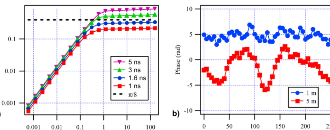
The integral of Eq. (22) was numerically evaluated for different values of τ, and for different sampling times Δ. The detection bandwidth was set to 100 MHz. Figure 6(a) shows the resulting standard deviation of the phase difference as a function of the distance D, for the frequency noise of VCSEL sample #1. We note that the standard deviation is always smaller than π/8 for a sampling time < 1.6 ns. Even more remarkably, the standard deviation is almost stable for distances larger than 1 m, and approaches asymptotically an upper limit. In these conditions, the maximal measurable distance is therefore theoretically unlimited. This asymptotic limit can be explained as follows: as already mentioned, the interferometer acts as a moving average over the time window τ. This moving average process becomes dominant compared to the detection low-pass filter detection as soon as 1/τ < B. If the sampling time Δ is shorter than the interferometric delay τ, consecutive samples become correlated. Under these conditions, the phase noise increases with increasing distances D, but on the other hand, consecutive samples are getting more and more correlated. This property is illustrated in Fig. 6(b). Although the phase noise is higher at 5 m, the correlation time of the phase noise sequence is clearly longer compared to the one at 1 m. Consequently, the standard deviation of the phase difference between consecutive samples becomes constant at long distances.

-10 -5 0 5 10 Ph as e (r ad ) 250 200 150 100 50 0 Time (ns) 1 m 5 m 0.001 0.01 0.1 P ha se d iff er en ce s td ev (ra d) 0.001 0.01 0.1 1 10 100 Distance D (m) 5 ns 3 ns 1.6 ns 1 ns π/8 a) b)

Fig. 6. (a) Standard deviation of the phase difference between consecutive samples as a function of the distance D, for B = 100 MHz. (b) Phase noise sequences, generated by Monte-Carlo simulations at two different distances D, for B = 100 MHz and Δ = 5 ns.

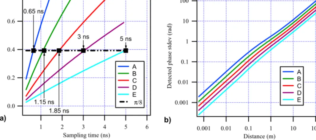
Figure 7(a) shows the standard deviation of the phase difference calculated at a distance of 1 km (i.e. very close to the asymptotic limit) as a function of the sampling time, and for different frequency noise PSDs. Table 2 shows the parameters C0, C1 and α that we

considered for these simulations. Case C corresponds actually to the VCSEL sample #1. For each case, the linewidth was estimated in the same way as those of the two VCSEL samples (see section 2.2), and Monte-Carlo simulations were realized to verify that Eqs. (16)-(18) are still valid. It turned out that the minimal required bandwidth B must be at least twice the linewidth of the laser, as indicated in Table 2. As shown in Fig. 7(a), the sampling time that is required to get a standard deviation smaller than π/8 ranges from 0.65 ns to 5 ns, depending on the frequency noise PSD. Figure 7(b) shows the standard deviation of the phase fluctuations that are expected, provided that these sampling time requirements are fulfilled.

0.001 0.01 0.1 1 10 100 Detec ted ph as e st dev (rad) 0.001 0.01 0.1 1 10 100 Distance (m) A B C D E 0.6 0.4 0.2 0.0 Phas e di fference s tdev (ra d) 6 5 4 3 2 1 Sampling time (ns) A B C D E π/8 0.65 ns 1.15 ns 1.85 ns 3 ns _{5 ns} a) _b)

Fig. 7. (a) Standard deviation of the phase difference vs sampling time and (b) standard deviation of the detected phase as a function of the distance D for the 5 different frequency noise PSDs and bandwidths listed in Table 2.

Table 2. Parameters used to calculate the curves of Fig. 7

Case

Frequency noise PSD Linewidth Bandwidth C0 (Hz) C1 (Hz1+α) α Δν (MHz) Β (MHz) A 1.5·107 _3.0·1014 _{1.1 100 200} B 7.6·106 _1.5·1014 _{1.1 70 140} C 3.8·106 _7.4·1013 1.1 ₅₀ 100 D 1.9·106 _3.7·1013 _{1.1 35 70} E 9.5·105 _1.9·1013 _{1.1 25 50} 4. Experimental verification 4.1 Set-up description

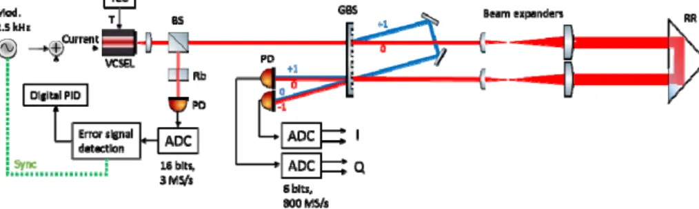
We experimentally tested the performance of a Michelson-type interferometer beyond the coherence length of the VCSEL laser source. The set-up is shown in Fig. 8. The VCSEL is of the same type as the VCSEL that served for the frequency noise measurement (VCSEL from ULM Photonics, part number ULM780-01-TN). The beam is first collimated with a diameter of about 0.6 mm. A first beamsplitter reflects one part of the beam towards an atomic absorption cell. The laser optical frequency is locked to a Doppler-broadened absorption line of natural rubidium (Rb) vapor. For sake of miniaturization, we use a micro-fabricated Rb vapor cell whose manufacturing technology is based on anodic bonding of silicon and glass wafers [13]. The evaluation of the frequency stability of a VCSEL locked to the same type of vapor cell has been reported in [14], showing relative instabilities lower than 10−9_{. The}

miniature vapor cell is heated to 80°C, by means of two glass windows coated with indium tin oxide (ITO). The digital stabilization loop will be described in more details in section 4.3. The beam transmitted by the beamsplitter enters then a modified Michelson interferometer, with two quadrature interference signals. To simplify the concept shown in Fig. 1, a custom designed grating beamsplitter is used to generate two 90° phase shifted signals, instead of the polarizing beam splitter, quarter waveplate, and polarizers. The + 1 diffraction order of the input beam is launched in the reference arm (in blue), and the 0 order propagates over the measurement arm (in red). After reflection, the two beams are recombined by the same diffraction grating. The 0 diffraction order of the measurement beam overlaps the + 1 order of the reference beam, and the 0 order of the reference beam overlaps the −1 order of the measurement beam, generating thus two interference signals. The geometry of the diffractive grating can be optimized in order to introduce a phase shift of 90° between these two signals. A similar approach is described in [15], although two harmonically-matched gratings were

used instead of a single custom-designed grating. Note that the laser beam which propagates towards the measurement retroreflector is expanded by a factor 10 using two lenses, to get a highly collimated beam with a diameter of 6 mm. The retro-reflected beam is in turn shrunk by the same factor using an identical two-lens system in order to match the reference beam. The two interference signals are detected by two custom-designed 130 MHz bandwidth photodetectors. As shown in Fig. 5(a), this bandwidth is high enough to prevent any 2π phase jump, provided that the sampling time is short enough.

Fig. 8. Optical layout of the experimental set-up for interferometric measurements beyond the coherence length. TEC: thermoelectric temperature control, BS: beamsplitter, Rb: rubidium cell, PD: photodetector, GBS: grating beamsplitter, RR: retroreflector, ADC: Analog-to-digital converter, PID: proportional–integral–derivative controller.

4.2 Signal processing

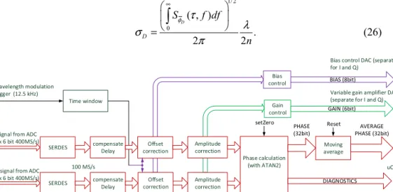
As shown in Fig. 8, the two interference signals I and Q are acquired at a sampling rate of 800 MS/s. The corresponding sampling time of 1.25 ns is short enough to avoid any phase unwrapping issue with the VCSEL that we used, according to Fig. 7(a) (case C). A dual 6-bit analog-to-digital converter (MAX105) is used for that purpose. Each channel provides actually two 6-bit data delayed by 1.25 ns, at an output data rate of half the sampling rate, i.e. 400 MS/s. I and Q data are then processed in a high-speed field programmable gate array (FPGA) circuit (Xilinx Virtex 6). The block diagram of the signal processing is shown in Fig. 9. To enable the processing at the required speed with an acceptable frequency clock of the FPGA, serial-to-parallel converters (SerDes [16]) are used at the inputs, to convert the four serial data at 400 MS/s into sixteen parallel data at 100 MS/s. The goal of the next functional block is to fine-tune the data delays, to accurately realign the I and Q signals. In order to be able to calibrate offsets and amplitudes of the interference signals, the frequency of the VCSEL laser is modulated by acting on the injection current, at a modulation frequency f of 12.5 kHz (see Fig. 8). The interference signal becomes therefore of the form

[

]

{

}

( ) cos 2 cos(2 ) i( , ) .

S t = +A B π ν+ Δν π ft τ φ τ+ t (23)

We chose a modulation amplitude Δν of 7.5 GHz, so that at least one maximum and one minimum of interference is scanned at the minimal distance of 1 cm. Under these conditions, the amplitudes and offsets of the two interference signals can be easily calibrated and compensated in the signal processing. We can also directly act on the offset subtraction stage of the transimpedance amplifiers and on the variable gain amplifiers in order to adapt the input signal ranges to the range of the ADC. The phase is then estimated using a look-up-table which emulates the atan2 operation between I and Q data, before its unwrapping operation. A moving average over the modulation period (80 μs) is then performed to remove the phase modulation. This corresponds to an average over 64’000 consecutive samples. The 32-bit average phase ͞φD is finally converted into distance using the relation

, 2 2 D D n φ λ π = (24)

where n is the refraction index of air. Note that we can take the moving average over T = 80 μs into account in the expression of the PSD of the detected phase by multiplying Eq. (16) with the function sinc2_{(πfT). Using Eqs. (8), (9), (16) and (17), and since T is much longer}

than τ and 1/B, we finally get

(

)

(

)

The expected standard deviation of the distance D can be calculated from the variance of ͞φD, which can be found from the integration of Eq. (25):

1/ 2 0 ( , ) . 2 2 D D S f df n φ τ _λ σ π ∞       =



I-signal from ADC (2x 6 bit 400MS/s)

Q-signal from ADC

(2x 6 bit 400MS/s) _DIAGNOSTICS Time window uC compensate Delay compensate Delay Amplitude correction Reset

Bias control DAC (separate for I and Q)

Variable gain amplifier DAC (separate for I and Q)

100 MS/s Amplitude correction Gain control BIAS (8bit) Bias control

Fig. 9. Block diagram of the interferometer signal processing, implemented in a Virtex 6 FPGA circuit.

4.3 Frequency stabilization

The absorption signal is detected and digitized using an ADC working at 3 MS/s (16-bit), and then processed in the FPGA. Since the frequency modulation width (15 GHz) is much wider than the absorption linewidths (about 500 MHz FWHM), we had to implement a non-standard stabilization technique. The goal of the stabilization is to lock the zero crossing of the frequency modulation signal to the center of one of the Rb absorption lines. For that purpose, two time windows of equal duration (2 μs) are generated just before and after the zero crossing, as shown in Fig. 10. The absorption signals are numerically integrated during each time window, yielding two summation results. The difference between these two last values is proportional to the first derivative of the absorption line shape with respect to the laser frequency. The value of the first derivative goes to 0 when the mean laser frequency ν0 is

equal to the center of the absorption line νabs, and changes sign whenever (ν0 – νabs) changes sign. Therefore, the subtraction between the two summation results is an appropriate error signal for the stabilization loop. This error signal feeds then a PID controller which is implemented in the firmware of a microcontroller.

-10 0 10 Cu rre n t ( μ A) 80x10-6 60 40 20 0 Time (s) 1.0 0.5 0.0 T im e w indow 1.0 0.8 0.6 0.4 0.2 0.0 Intensity ( a .u.) Time window #1 Time window #2

Fig. 10. Timing diagram for the frequency stabilization. The upper graph is the current modulation added to the DC injection current of the VCSEL. The medium graph shows the time windows that are generated by the FPGA, synchronized to the modulation signal. The absorption signal (shown in the lower graph) is integrated during these two time windows yielding the two areas represented in red and blue. The goal of the stabilization is to balance these two areas.

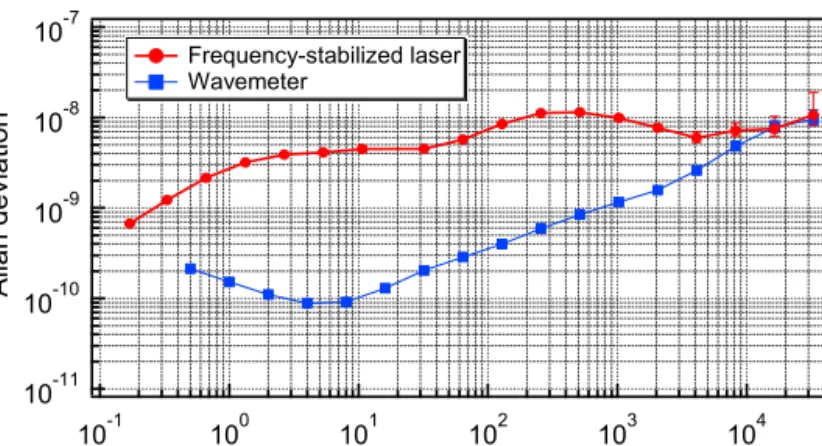
10-11 10-10 10-9 10-8 10-7 Allan deviation 10-1 100 101 102 103 104 Integration time [s] Frequency-stabilized laser Wavemeter

Fig. 11. Fractional frequency stability in terms of Allan deviation of the VCSEL locked to natural Rb (red) and of the wavemeter used to evaluate the stability of this laser source (blue).

The wavelength stability provided by this digital stabilization loop was estimated by means of a high-accuracy wavemeter (Toptica HighFinesse WSU-10). The Allan deviation was estimated for different integration times. The wavemeter was first calibrated with a reference laser stabilized onto Rb in a sub-Doppler absorption scheme whose frequency stability is better than 10−11 _{at all timescales from 1 s up to 1 day. A relative stability ≤ 10}−8

was demonstrated for integration times between 0.1 s to 30’000 s, as illustrated in Fig. 11. Above 10’000 s, the stability measurement is limited by the drift of the wavemeter. In free-running regime, the frequency stability of an equivalent VCSEL operating at 894 nm was reported at the level of 10−8 _{at 1 s and 5·10}−7 _{at 100 s [17].}

4.4 Experimental results

The interferometer prototype was mounted on a test bench for interferometric measurements over long distances. The measurement retroreflector was mounted on a test carriage, whose position along a rail is controlled using an absolute distance meter (ADM) located at the opposite side, as depicted in Fig. 12. The ADM is a device that is integrated in absolute laser trackers from Leica Geosystems [18]. The measurement beam of the ADM is directed towards another retroreflector mounted on the same carriage. The positioning resolution is 3.8 μm. The short-term stability of the interferometric test bench was first characterized by means of an Agilent interferometer. The standard deviation of the distance variations was estimated to be 0.035 μm at short distances. These variations are probably caused by mechanical vibrations of the set-up.

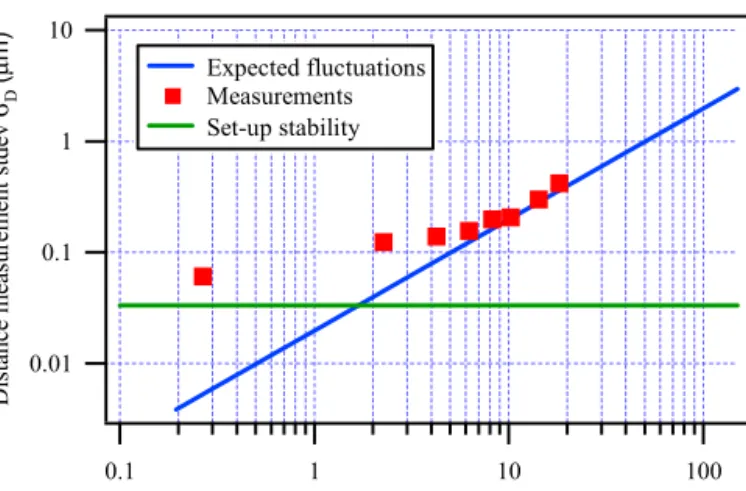
Fig. 12. Test bench used for the experimental verification. ADM: Absolute distance measurement device. 0.01 0.1 1 10 D is tance meas ur ement s tdev σD ( μ m) 0.1 1 10 100 Distance D (m) Expected fluctuations Measurements Set-up stability

Fig. 13. Standard deviation of the distance measurement fluctuations, as a function of the distance D. The expected fluctuations are calculated from Eq. (26).

Thanks to this test bench, we could operate the VCSEL interferometer prototype at different distances D ranging from 0.25 m to 18 m. We never observed any 2π phase jump over this range. The agreement between ADM and the VCSEL displacement measurements was better than 4.5 ppm. The accuracy determination was unfortunately limited by slow drifts, probably caused by the different environmental conditions seen by the ADM and the VCSEL beams (gradient of temperature, air turbulence), since both beams don’t share the same optical path. The interferometer results were acquired during 1 min at 8 positions between 0.25 m and 18 m. The slow drifts caused by mechanical instabilities have been compensated, and the standard deviation was then calculated. The resulting values were compared to the ones predicted by Eq. (26), with T = 80 μs, fc = 1 kHz, and the frequency noise measured on sample #1 (see Table 1). Results are shown in Fig. 13. As expected, the mechanical vibrations of the interferometric set-up limit the resolution at short distances. At longer distances, the distance fluctuations become larger with increasing distances, with a slope of about 0.02

μm/m. From 6 m to 18 m, the measured values are in good agreement with the values predicted with Eq. (26).

Conclusion

We demonstrated theoretically and experimentally that the coherence length of the source is no more a fundamental limit for interferometric measurements, thanks to modern high-speed digital processing implemented in FPGA. By measuring the interference signals with high bandwidth photodetectors, the interference contrast is not any more reduced beyond the coherence length, although the signal becomes affected by a strong phase noise. This phase noise can be measured, provided that the sampling time is sufficiently short to prevent any phase unwrapping issues. Under some conditions, the maximal distance that can be measured is theoretically infinite. Indeed, even if the phase noise amplitude becomes larger for increasing distances, the cut-off frequency of the low-pass filter caused by the interferometer becomes lower, thus smoothing the phase noise. The phase difference between successive samples becomes constant beyond the coherence length of the laser.

Using a frequency stabilized VCSEL, we could measure displacements up to 18 m, corresponding to an optical path difference of 36 m. This is at least five times longer than the coherence length of the laser which lies between 3 m to 6.6 m (depending on the samples), according to the measurements of frequency noise and linewidths. After phase noise averaging over 80 μs, the 3σ distance fluctuations are lower than 1.2 μm at a distance of 18 m, corresponding to a relative stability better than 0.1 ppm. These performances are competitive compared to standard industrial interferometers, which are usually based on He-Ne laser. The possibility to overcome the coherence length opens therefore the way for long displacement measurements using miniature interferometers based on inexpensive semiconductor laser sources.

Funding

Swiss Commission for Technology and Innovation (CTI) (Project no 12344.1 PFNM-NM); Hexagon Technology Center GmbH.

Acknowledgments

We would like to thank Laure Jeandupeux and Francois Feuvrier (Haute Ecole ARC Ingenierie) for the manufacturing of the grating beamsplitter, and Rainer Wohlgenannt (Hexagon Technology Center) for the design of the analog part of the electronic board. We are also grateful to Yves Petremand (Centre Suisse d’Electronique et de Microtechnique, CSEM) for providing the miniature Rb absorption cells.