HAL Id: tel-03254461
https://tel.archives-ouvertes.fr/tel-03254461
Submitted on 8 Jun 2021
HAL is a multi-disciplinary open access
archive for the deposit and dissemination of
sci-entific research documents, whether they are
pub-lished or not. The documents may come from
teaching and research institutions in France or
abroad, or from public or private research centers.
L’archive ouverte pluridisciplinaire HAL, est
destinée au dépôt et à la diffusion de documents
scientifiques de niveau recherche, publiés ou non,
émanant des établissements d’enseignement et de
recherche français ou étrangers, des laboratoires
publics ou privés.
Post-quantum cryptography: a study of the decoding of
QC-MDPC codes
Valentin Vasseur
To cite this version:
Valentin Vasseur. Post-quantum cryptography: a study of the decoding of QC-MDPC codes.
Cryp-tography and Security [cs.CR]. Université de Paris, 2021. English. �tel-03254461�
Université de Paris
École doctorale Informatique, Télécommunications et Électronique de Paris
Inria équipe-projet COSMIQ
Post-quantum cryptography:
a study of the decoding of
QC-MDPC codes
Cryptographie post-quantique :
étude du décodage des codes QC-MDPC
Par Valentin Vasseur
Thèse de doctorat d’informatique
Dirigée par Nicolas Sendrier
Présentée et soutenue publiquement le 29 mars 2021 Devant un jury composé de :
Nicolas Sendrier Inria Directeur
Jérôme Lacan ISAE-Supaero Rapporteur
Pierre Loidreau Université de Rennes Rapporteur
Alain Couvreur Inria Examinateur
Caroline Fontaine ENS Paris-Saclay Examinatrice Philippe Gaborit Université de Limoges Examinateur Sophie Laplante Université de Paris Examinatrice
Équipe-projet COSMIQ Inria,
2 rue Simone Iff, 75 012 Paris
Remerciements
Je dois d’abord remercier mon directeur de thèse, Nicolas, de m’avoir proposé de travailler sur cet algorithme si simple à décrire, mais qui a conduit à tant de questionnements et qui m’a permis de découvrir un domaine si riche. Merci pour ta disponibilité, tes explications, tes conseils et ton humour.
Je remercie Jérôme Lacan et Pierre Loidreau d’avoir accepté d’être rapporteurs. Je remercie également Alain Couvreur, Caroline Fontaine, Philippe Gaborit, Sophie Laplante et Jean-Pierre Tillich d’avoir accepté de faire partie du jury.
Il règne toujours une très bonne ambiance au sein de l’équipe SECRET/COSMIQ, merci donc à Anne, André, Pascale, Gaëtan, Anthony, María, Léo, Nicolas, Jean-Pierre et Christelle. Bien évidemment, je remercie aussi ceux qui étaient de passage dans l’équipe et ceux qui sont de passage aujourd’hui (en espérant n’oublier personne, la liste est longue) : Magali, Augustin, Yann, Xavier, Christina, Clémence, Pierre, Rémi, Étienne, Rodolfo, Kevin, Kaushik, Julia, Daniel, Nicolas, Thomas, Loïc, Aurélie, Sébastien, Simona, Antonio, Paul, Antoine, Lucien, Vivien, Johana, Rocco, Andrea, Clara, Yann, André et Christophe. Je pourrais même ajouter Étienne, Thierry et Bernard qui font presque partie de l’équipe. Et bien sûr, je n’oublie pas les membres du bureau Tapdance canal historique Mathilde, Matthieu et Ferdinand qui par leur bonne humeur ont contribué à ce que ce soit toujours un plaisir de venir au bureau.
Je remercie toutes les personnes que j’ai rencontrées au cours de ces dernières années et avec lesquelles je partage de bons souvenirs. Merci donc tout d’abord à Moran, Sonia, Lolo, Cyril, Céline, Benjamin, Clément, Marion et Vincent puis Caro, Cindy, Nico et Quentin et enfin Pascal, Pauline et Louis.
Je tiens à remercier Daniel Agier qui a réussi à me passionner pour les mathématiques dès le lycée.
Pour finir, merci à ma famille proche qui me tolère depuis toutes ces années. Merci à Mumu sans qui je serais probablement à la rue en ce moment ou pire, en banlieue. Merci à mes parents qui m’ont permis de faire ces études si longues mais passionnantes. Les contraintes du calendrier font que je soutiens ma thèse le jour d’un bien triste anniversaire, mais je sais que tu aurais été fière que ton fils soit docteur.
Contents
Introduction
1
Notations
5
I Preliminaries
7
1 Coding theory 9 1.1 Linear codes. . . 9 1.2 Decoding . . . 101.3 Minimum distance & Gilbert-Varshamov distance. . . 11
1.4 Regularity . . . 11
1.5 Channel . . . 12
1.6 Schur product. . . 12
1.7 (QC-)MDPC codes and basic properties . . . 13
2 Security reduction 15 2.1 Security games . . . 16
2.2 Fujisaki-Okamoto transform . . . 16
3 Code-based cryptography 19 3.1 McEliece cryptosystem framework . . . 19
3.2 Niederreiter cryptosystem framework . . . 20
3.3 Best known attacks on underlying hard problems . . . 20
4 BIKE 25 4.1 Security . . . 26
4.2 Block size . . . 28
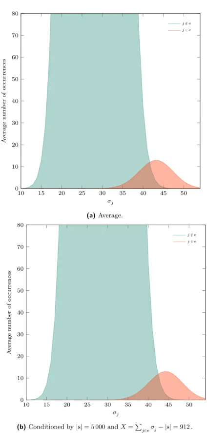
5 Syndrome weight and counters in a regular MDPC code 31 5.1 Fundamental quantities . . . 31
5.2 Counters distributions . . . 32
5.2.1 Average case . . . 33
5.2.2 Conditioning the counter distributions with the syndrome weight . 33
II New bit-flipping decoders for QC-MDPC
37
6 Introduction 41 6.1 State of the art . . . 416.1.1 LDPC codes . . . 42
6.1.2 MDPC codes . . . 47 iii
6.1.3 QC-MDPC decoding thresholds. . . 48 6.2 Contributions . . . 49 7 Step-by-step 53 7.1 Definition . . . 53 7.2 Sampling positions . . . 53 7.2.1 Uniform sampling . . . 54
7.2.2 Picking a position in one unsatisfied equation . . . 54
7.2.3 Picking a position in two unsatisfied equations . . . 55
7.3 Performance. . . 57
7.4 Non-blocking variant . . . 58
8 Backflip 61 8.1 Algorithm description . . . 61
8.2 Threshold and time-to-live. . . 62
8.2.1 Optimistic threshold strategy . . . 63
8.2.2 Multiple thresholds strategy . . . 65
9 Gray decoders 67 9.1 Framework . . . 67
9.2 Reverifications . . . 67
9.3 Simple definition . . . 68
9.4 Variants from Drucker, Gueron & Kostic . . . 69
9.5 Sorting variant . . . 70
III Analysis of bit-flipping decoders for QC-MDPC
77
10 Introduction 81 10.1 State-of-the-art . . . 8110.1.1 LDPC codes . . . 81
10.1.2 Expander codes arguments . . . 82
10.1.3 Analysis of regular LDPC codes with a bit-flipping algorithm . . . 83
10.1.4 MDPC codes . . . 83
10.2 Contributions . . . 87
11 One iteration of the parallel decoder with variable thresholds 89 11.1 Notations . . . 90
11.2 Mass equations in regular codes. . . 91
11.3 Modeling the error weight after the first iteration . . . 93
11.3.1 Estimating the number of errors per equation . . . 93
11.3.2 Estimating the syndrome weight and the sum of the counters . . . 93
11.3.3 Counters distributions . . . 95
11.3.4 Predicting flips . . . 97
11.3.5 Error weight after one iteration . . . 101
11.3.6 Unconditional probability of the error weight after the first iteration 101 11.4 A two-iteration decoder with a DFR analysis . . . 103
11.4.1 One iteration . . . 103
11.4.2 Two iterations . . . 103
11.4.3 Decoding performance requirements after the first iteration . . . . 107
11.5 Noisy syndrome decoding . . . 108
12 Markovian model of the step-by-step algorithm 113
12.1 Notations . . . 113
12.2 Algorithm supported by the model . . . 114
12.3 Assumptions . . . 114
12.4 DFR estimation within the model. . . 116
12.5 Transition probabilities . . . 117
12.5.1 Blocked state . . . 118
12.5.2 Transitions from a non-blocked state . . . 118
12.6 Results. . . 119
12.6.1 Using the step-by-step decoder only . . . 120
12.6.2 Using the step-by-step decoder for residual error correction . . . . 120
IV Practical DFR estimation
123
13 Introduction 127 13.1 State-of-the-art . . . 12713.1.1 Designing good LDPC code . . . 127
13.1.2 Error floors in LDPC codes . . . 127
13.1.3 DFR and spectrum of QC-MDPC codes . . . 128
13.1.4 Weak keys in a QC-LDPC cryptosystem . . . 128
13.1.5 Weak keys in QC-MDPC cryptosystems . . . 129
13.2 Contributions . . . 129
14 A DFR extrapolation framework 131 14.1 Notations . . . 131
14.2 The decoder security assumption . . . 131
14.3 Security of the system with respect to the block size . . . 132
14.4 Confidence interval . . . 133
14.5 A first estimation. . . 134
14.5.1 Clopper-Pearson interval. . . 134
14.5.2 A first estimation of confidence intervals for extrapolations . . . . 134
14.6 Using posterior probability . . . 135
14.7 Choosing parameters . . . 137
15 Weak keys: Subsets of parity check matrices 141 15.1 QC-MDPC Codes . . . 141
15.1.1 Definition and polynomial representation . . . 141
15.1.2 Decoding . . . 142
15.2 Notations . . . 142
15.3 Distance Spectrum . . . 143
15.3.1 New properties of the distance spectrum . . . 143
15.3.2 Distance spectrum statistics . . . 144
15.3.3 Reconstructing the secret key from the spectrum . . . 146
15.4 Weak keys: Constructions and properties . . . 147
15.4.1 IND-CCA security and weak keys for KEMs. . . 147
15.4.2 Type I . . . 148
15.4.3 Type II . . . 149
15.4.4 Type III . . . 151
15.4.5 Statistics . . . 151
15.5 DFR estimations . . . 151
16 Error floors: Subsets of error patterns 157
16.1 Notations . . . 159
16.2 Structured patterns in QC-MDPC codes . . . 159
16.2.1 Low weight codewords . . . 159
16.2.2 Near-codewords. . . 160
16.3 Error patterns impeding decoding. . . 160
16.4 Lower bound on the DFR with simulations . . . 163
16.5 Comments. . . 163
Introduction
Most cryptosystems in use today rely on the hardness of number theory problems such as the factorization or the discrete logarithm problems, either in finite fields or in elliptic curves. These problems with the current parameters would not resist an adversary with a sufficiently powerful quantum computer [Sho99; Joz01]. In fact the security of these problems would scale poorly against such an adversary, see for example [BHLV17].
In anticipation of the development of a powerful quantum computer, alternatives to cryptosystems based on number theory are gaining momentum in research. The National Institute of Standards and Technology (NIST) launched in 2014 a process1 to standardize
the first post-quantum public key encryption (PKE), key encapsulation mechanisms (KEM) and signatures. Initially, 82 proposals were submitted. At the time of writing, we are in the 3rd round and there are 7 finalists in the running, most likely candidates for standardization in the short term, and 8 alternate candidates, who may need another round of evaluation. The breakdown by domain of the remaining proposals is presented in Table1.
Table 1: NIST Post-Quantum Cryptography Standardization Process — Round 3
PKE/KEM Signature Finalists Code 1 0 Lattice 3 2 Multivariate 0 1 Alternate candidates Code 2 0 Lattice 2 0 Hash 0 1 Isogeny 1 0 Multivariate 0 1 Zero-knoweldge 0 1
We can see that the proposed cryptosystems are based on problems that cover a wide range of mathematical fields. Let us focus on code-based cryptography. The only code-based finalist in the NIST standardization process is based on [McE78], published in 1978 in which McEliece introduced the idea of using error-correcting codes in cryptography.
Error correcting codes are extensively used in telecommunications. To transmit a message, it is first transformed into a codeword, a process that adds redundancy. If the codeword is transmitted over a noisy channel, it will contain errors when it reaches its recipient. Redundancy implies that we are still able, as long as the number of errors is limited, to recover the original message from this noisy codeword. A good error-correcting
1https://csrc.nist.gov/projects/post-quantum-cryptography
code has a certain structure that makes it possible to have an efficient decoder, that is to say, an algorithm that removes many errors in a timely manner. On the other hand, a random code is hard to decode.
McEliece had the idea of hiding a message by taking the corresponding codeword and adding as many errors as it is possible to remove. He used Goppa codes. On the one hand, they have good decoders, which allows decryption. And on the other hand, once scrambled, these codes are hard to distinguish from random codes. So anyone who does not know how the code was scrambled will not have a good decoder. In other words, we have a public-key encryption system: if the scrambled code is made public, anyone can use it to encrypt, but only the person who knows how it was scrambled can decrypt.
It is remarkable that, so far, this system has not been affected by any major attack, classical or quantum, and that it is now being considered for standardization. However, the public key size is in the order of a few megabits. This can be a hindrance for some applications. In order to reduce the key size, one can therefore consider using codes other than Goppa codes. Many attempts have been made in this direction and most of them have resulted in broken cryptosystems.
The Quasi-Cyclic Moderate Density Parity Check (QC-MDPC) codes, proposed in [MTSB13], appear to be good candidate for replacing Goppa codes in a McEliece cryptosystem. They have small key sizes and have not suffered major attacks. However, unlike Goppa codes, the principle of their decoder does not depend on algebraic properties but on probabilistic properties. Consequently, decoding may fail.
It has been shown in [GJS16] that the decoder leaks information about the secret key in case of failures. In fact, when the same key is used, an adversary who encrypts a large number of messages and has the ability to determine which ones failed to decrypt, can retrieve the secret key from the set of these failure-triggering messages. Thus, to use keys that are not ephemeral but static, it is necessary to ensure that the decoding failure rate (DFR) is very low. This is also a necessary condition to be able to verify strong security constraints such as indistinguishability under chosen ciphertext attack (IND-CCA).
QC-MDPC decoders and their DFR are the primary focus of the works presented in this document. Our motivation is threefold: to improve decoding algorithms, to better understand their workings and to ensure that they fail with negligible probability. We will focus on [BIKE] a Key Encapsulation Mechanism that uses QC-MDPC codes. It is an alternate candidate to the NIST Post-Quantum Cryptography Standardization Process.
NIST has expressed concerns about its IND-CCA security and DFR analysis in [Ala+20], but nonetheless considers it one of the most promising candidates. This document is a step toward addressing these concerns.
This document is divided in four parts.
The first part recalls the necessary background on coding theory, public key cryptography,
security reductions, code-based cryptography and the specificities of the QC-MDPC based scheme BIKE.
The second part presents new decoding algorithms and reviews some aspects of their
implementation. The performance and tuning of these algorithms will be discussed from an essentially empirical point of view.
The third part describes two theoretical probabilistic models for some MDPC decoders,
the ultimate goal being to predict their DFR.
The fourth part introduces a new decoding assumption and the statistical framework it
implies for extrapolating the DFR from simulation measurements. We then study specific parity check matrices or error patterns that, due to the structural properties of QC-MDPC codes, are great candidates to challenge this new assumption.
Publications
[BIKE] Carlos Aguilar Melchor, Nicolas Aragon, Paulo S L M Barreto, Slim Bettaieb, Loïc Bidoux, Olivier Blazy, Jean-Christophe Deneuville, Philippe Gaborit, Ghosh Santosh, Shay Gueron, Tim Güneysu, Rafael Misoczki, Edoardo Persichetti, Nicolas Sendrier, Jean-Pierre Tillich, Valentin Vasseur, and Gilles Zémor. BIKE. NIST Round 3 submission for Post-Quantum Cryptography. Aug. 2020. url:https://bikesuite.org.
[SV19] Nicolas Sendrier and Valentin Vasseur. “On the Decoding Failure Rate of QC-MDPC Bit-Flipping Decoders”. In: Post-Quantum Cryptography (PQCrypto). Ed. by Jintai Ding and Rainer Steinwandt. Vol. 11505. LNCS. Chongqing, China: Springer, May 2019, pp. 404–416. doi: 10.1007/978-3-030-25510-7_22.
[SV20a] Nicolas Sendrier and Valentin Vasseur. “About Low DFR for QC-MDPC Decoding”. In: Post-Quantum Cryptography (PQCrypto). Ed. by Jintai Ding and Jean-Pierre Tillich. Vol. 12100. LNCS. Paris, France: Springer, Apr. 2020, pp. 20–34. doi:10.1007/978-3-030-44223-1_2.
[SV20b] Nicolas Sendrier and Valentin Vasseur. On the existence of weak keys for
QCMDPC decoding. Cryptology ePrint Archive, Report 2020/1232. 2020.
Notations
General.
• Vectors and polynomials are denoted in roman type (e.g. h) and matrices in bold (e.g. H).
• The support Supp(v) of a vector v is the set of indices of its nonzero entries. [Def.1.15p. 11] • The weight |v| of a vector v is always the Hamming weight. [Def.1.16p. 11] • The vector operator ⋆ is the Schur product, both for vectors and polynomials.
[Def.1.24p. 12] • The notation 𝑥← 𝑆$ means drawing uniformly at random an element from 𝑆 and
assign it to 𝑥.
Coding theory.
• The following variables are restricted to the following usage unless stated otherwise:
– 𝑛: the length of a code; – 𝑘: the dimension of a code;
– 𝑟 = 𝑛 − 𝑘: the dimension of the dual; the block size of a quasi-cyclic parity
check matrix;
– 𝑑: the column weight of a parity check matrix; – 𝑤: the row weight of a parity check matrix; – 𝑡: the weight of an error pattern.
• For all 𝑗 ∈ {0, … , 𝑛 − 1}, 𝜎𝑗∶= ∣h𝑗⋆s∣ . [Def.5.1p. 31]
• For a matrix H, we denote its 𝑖-th row by h⊺
𝑖, and its 𝑗-th column by h𝑗.
• We will represent information vectors m, error patterns e and codewords c as row vectors; and the syndrome s as a column vector:
G ∈ 𝔽𝑘×𝑛
𝑞 , H ∈ 𝔽 (𝑛−𝑘)×𝑛
𝑞 , c = mG , s = He⊺.
H s 𝑛 − 𝑘 = 𝑟
𝑛
Part I
Preliminaries
Chapter 1
Coding theory
In this chapter we will recall the fundamental notions from coding theory that we will need to construct QC-MDPC codes.
1.1 Linear codes
Definition 1.1. Let 𝑘 and 𝑛 be two positive integers with 𝑘 ≤ 𝑛. An 𝔽𝑞-linear code 𝒞 of
length 𝑛 and dimension 𝑘 is a linear subspace of dimension 𝑘 of the vector space 𝔽𝑛 𝑞.
Such a code is designated as an [𝑛, 𝑘]-code.
Definition 1.2. The rate of a code 𝒞 of dimension 𝑘 and length 𝑛 is the ratio
𝑅 = 𝑘 𝑛.
In the context of telecommunications, when using an [𝑛, 𝑘]-linear code to send infor-mation, for every 𝑘 symbols of useful inforinfor-mation, (𝑛 − 𝑘) redundant symbols are also sent. The code rate is therefore the proportion of useful information that is sent through a channel. The reduntant information is used for error-detection and correction.
Definition 1.3. A matrix G ∈ 𝔽𝑘×𝑛
𝑞 is said to be a generator matrix of the linear code 𝒞 if
its rows form a basis of 𝒞.
Definition 1.4. The dual code 𝒞⟂⊂ 𝔽𝑛
𝑞 of a code 𝒞 is the orthogonal space
𝒞⟂∶= {v ∈ 𝔽𝑛
𝑞 | ∀w ∈ 𝒞, v ⋅ w = 0}
where v ⋅ w is the scalar product ∑𝑛−1 𝑖=0 𝑣𝑖𝑤𝑖.
A generator matrix for the dual code 𝒞⟂ is called a parity check matrix for 𝒞.
We will call equations the rows of parity check matrix.
Definition 1.5. The generator matrix G (resp. the parity check matrix H) of a linear
code 𝒞 (of dimension 𝑘 and length 𝑛) is said to be in systematic form if is written as
G = [I𝑘 𝑃 ] resp. H = [I𝑛−𝑘 𝑃 ] .
Remark 1.6. A code is fully defined by its dual, therefore if H ∈ 𝔽(𝑛−𝑘)×𝑛
𝑞 is a parity check
matrix for an [𝑛, 𝑘]-code 𝒞 then
𝒞 = {c ∈ 𝔽𝑛
𝑞 |Hc⊺=0} .
10 Chapter 1. Coding theory Remark 1.7. If G ∈ 𝔽𝑘×𝑛
𝑞 and H ∈ 𝔽 (𝑛−𝑘)×𝑛
𝑞 are respectively a generator and a parity check
matrices of a code 𝒞 then we have
HG⊺=0 .
Definition 1.8. Let 𝒞 be a code of length 𝑛 and dimension 𝑘 with parity check matrix H ∈ 𝔽(𝑛−𝑘)×𝑛
𝑞 . The syndrome of a vector x ∈ 𝔽𝑞𝑛 is the vector
Hx⊺∈ 𝔽𝑛−𝑘 𝑞 .
Definition 1.9. Let 𝒞 be a binary code of length 𝑛 and dimension 𝑘 with parity check
matrix H ∈ 𝔽(𝑛−𝑘)×𝑛
2 . We say that the 𝑖-th equation is satisfied if the corresponding
syndrome bit 𝑠𝑖 is zero, and we say that the equation is unsatisfied otherwise.
1.2 Decoding
Definition 1.10. Let 𝒞 be a code of length 𝑛 and dimension 𝑘 with generator matrix G ∈ 𝔽𝑘×𝑛
𝑞 and parity check matrix H ∈ 𝔽 (𝑛−𝑘)×𝑛 𝑞 .
Let x ∈ 𝔽𝑛
𝑞, decoding is the process of finding a vector e ∈ 𝔽𝑞𝑛 such that
x − e ∈ 𝒞 i.e. ∃m ∈ 𝔽𝑘
𝑞,x = mG + e .
Let s ∈ 𝔽𝑛−𝑘
𝑞 , syndrome-decoding is the process of finding a vector e ∈ 𝔽𝑞𝑛 such that
He⊺=s .
Remark 1.11. There exists different flavors of decoders, for example:
• a minimum distance decoder minimizes the Hamming weight of the vector e, • a maximum likelihood decoder finds m that maximizes Pr[x received | m sent] for a
specific channel.
Remark 1.12. In code-based cryptography we rely on the (syndrome) decoding problem in
which the challenge is to decode a given instance (see §3.3).
Definition 1.13. The Tanner graph of a binary parity check matrix H is the bipartite
graph defined by the biadjacency matrix H. If H ∈ 𝔽(𝑛−𝑘)×𝑛
2 , in the Tanner graph, the 𝑛 columns correspond to 𝑛 nodes called the
variable nodes, and the (𝑛 − 𝑘) rows correspond to (𝑛 − 𝑘) nodes called the check nodes.
While the use of the graph structure was already somehow practiced by Gallager in [Gal63], the notion was named after Tanner because of his work on the construction of long codes from smaller codes in [Tan81].
Related to the probalities computation in the Tanner graph, the following important classic result on the parity of a sum of binary random variables will be needed in this document (see [Gal63, Lemma 4.1] for a proof).
Proposition 1.14. Let 𝑘 be a positive integer, 𝑝1, … , 𝑝𝑘 ∈ [0, 1] and 𝑋1, … , 𝑋𝑘 be 𝑘
independent binary random variables following Bernoulli distributions with probabilities respectively 𝑝1, … , 𝑝𝑘. Then
∀𝑏 ∈ {0, 1},Pr[𝑋1+ ⋯ + 𝑋𝑘mod 2 = 𝑏] =
1 + (−1)𝑏∏𝑘
ℓ=1(1 − 2𝑝ℓ)
1.3. Minimum distance & Gilbert-Varshamov distance 11
1.3 Minimum distance & Gilbert-Varshamov distance
Definition 1.15. The support of a vector v ∈ 𝔽𝑛
𝑞 is the set of indices of its nonzero entries:
Supp(v) ∶= {𝑖 ∈ {0, … , 𝑛 − 1} ∣ 𝑣𝑖≠ 0} .
We use the same notation for polynomials Supp (𝑛−1∑
𝑖=0
𝑣𝑖𝑥𝑖) ∶= {𝑖 ∈ {0, … , 𝑛 − 1} ∣ 𝑣𝑖≠ 0} .
Definition 1.16. The Hamming weight |v| of a vector (or a polynomial) v is the number of
its nonzero entries
|v| ∶= ∣Supp(v)∣ .
The Hamming distance 𝑑(a, b) between two vectors a and b is the Hamming weight of the difference between a and b:
𝑑(a, b) ∶= |a − b| .
Definition 1.17. The minimum distance of a code 𝒞 is the minimum distance between
two distinct codewords:
min
c0,c1∈𝒞
c0≠c1
𝑑(c0,c1) .
Remark 1.18. For a linear code, we have
min c0,c1∈𝒞 c0≠c1 𝑑(c0,c1) =min c∈𝒞 c≠0 |c| .
Definition 1.19. Let 𝑞, 𝑛 and 𝑘 be integers. The Gilbert-Varshamov distance 𝑑𝐺𝑉(𝑞, 𝑛, 𝑘)
is the smallest integer 𝑑 such that
𝑑−1 ∑ 𝑖=0 (𝑛 𝑖)(𝑞 − 1) 𝑖≥ 𝑞𝑛−𝑘.
Remark 1.20. Let 𝑞, 𝑛 and 𝑘 be integers. For an [𝑛, 𝑘]-code drawn uniformly at random,
the expected number of possible solutions of weight below or equal to 𝑤 to a decoding problem is
∑𝑤𝑖=0(𝑛𝑖)(𝑞 − 1)𝑖
𝑞𝑛−𝑘 .
So, on average, there is one solution to a decoding problem with weight 𝑑𝐺𝑉(𝑞, 𝑛, 𝑘).
Definition 1.21. The binary entropy function is:
H(𝑋) ∶= H(𝑝) = −𝑝 log2𝑝 − (1 − 𝑝)log2(1 − 𝑝) .
1.4 Regularity
Definition 1.22. Let 𝑙 and 𝑟 be two positive integers. An (𝑙, 𝑟)-regular code is a code such
that, in its Tanner graph, every variable node has degree 𝑙 and every check node has degree 𝑟. The integers 𝑙 and 𝑟 are respectively the left and right degrees.
Equivalently if H is a parity check matrix, the code it defines is (𝑙, 𝑟)-regular if all its column have the same weight 𝑙 and all its rows have the same weight 𝑟.
12 Chapter 1. Coding theory
1.5 Channel
In telecommunications, when it comes to error correction, the model of the channel used is often specified. In cryptography, error patterns are often drawn uniformly at random among all fixed weight patterns. If a pattern has a weight 𝑡 and a length 𝑛, it can be seen, as a first approximation, as coming from a binary symmetric channel with a crossover probability 𝑡/𝑛.
Definition 1.23. Let 𝑥 be the binary random variable transmitted over a binary symmetric
channel of crossover probability 𝜖, let us write the received binary random variable 𝑦. Then
we have
Pr [𝑥 = 0 ∣ 𝑦 = 0] = Pr [𝑥 = 1 ∣ 𝑦 = 1] = 1 − 𝜖 , Pr [𝑥 = 0 ∣ 𝑦 = 1] = Pr [𝑥 = 1 ∣ 𝑦 = 0] = 𝜖 .
1.6 Schur product
Definition 1.24. The Schur product of two vectors v, w ∈ 𝔽𝑛
𝑞 is the componentwise product
v ⋆ w ∶= (𝑣0⋅ 𝑤0, 𝑣1⋅ 𝑤1, … , 𝑣𝑛−1⋅ 𝑤𝑛−1) .
We use the same notation for polynomials ( 𝑛−1 ∑ 𝑖=0 𝑣𝑖𝑥𝑖) ⋆ ( 𝑛−1 ∑ 𝑖=0 𝑤𝑖𝑥𝑖) ∶= 𝑛−1 ∑ 𝑖=0 (𝑣𝑖⋅ 𝑤𝑖)𝑥𝑖.
Proposition 1.25. The Schur product is distributive over the addition:
u ⋆ (v + w) = u ⋆ v + u ⋆ w .
Proposition 1.26. For any integer 𝑛 > 0, let 𝑣, 𝑤 ∈ 𝔽𝑛 2, then
|v + w| = |v| + |w| − 2 |v ⋆ w| .
Proof. v + v ⋆ w and w + v ⋆ w have disjoint support and weight respectively |v| − |v ⋆ w|
and |w| − |v ⋆ w|,
|v + w| = ∣(v + v ⋆ w) + (w + v ⋆ w)∣ .
Corollary 1.27. Let 𝑘 be a positive integer and let v1, … ,v𝑘 be 𝑘 vectors of equal length,
then ∣ 𝑘 ∑ 𝑖=1 v𝑖∣ = 𝑘 ∑ 𝑑=1 (−2)𝑑−1 ∑ 1≤𝑖1<⋯<𝑖𝑑≤𝑘 ∣v𝑖 1⋆ ⋯ ⋆v𝑖𝑑∣ .
Proof. Proposition1.26 shows the case where 𝑘 = 2. Now, let 𝑘 be any integer greater than 2, ∣ 𝑘 ∑ 𝑖=1 v𝑖∣ = ∣( 𝑘−1 ∑ 𝑖=1 v𝑖) + 𝑣𝑘∣ = ∣ 𝑘−1 ∑ 𝑖=1 v𝑖∣ + ∣𝑣𝑘∣ − 2 ∣ 𝑘−1 ∑ 𝑖=1 (v𝑖⋆v𝑘)∣ .
1.7. (QC-)MDPC codes and basic properties 13 Then, by induction hypothesis, we have
∣ 𝑘 ∑ 𝑖=1 v𝑖∣ = 𝑘−1 ∑ 𝑑=1 (−2)𝑑−1 ∑ 1≤𝑖1<⋯<𝑖𝑑−1≤𝑘−1 ∣v𝑖1⋆ ⋯ ⋆v𝑖𝑑−1∣ + ∣𝑣𝑘∣ − 2 𝑘−1 ∑ 𝑑=1 (−2)𝑑−1 ∑ 1≤𝑖1<⋯<𝑖𝑑−1≤𝑘−1 ∣v𝑖1⋆ ⋯ ⋆v𝑖𝑑−1⋆v𝑘∣ .
1.7 (QC-)MDPC codes and basic properties
Starting from this point in this document, we will only focus on binary codes (i.e. 𝔽2-linear
code).
Definition 1.28 (Low Density Parity Check). An [𝑛, 𝑘] LDPC code is a linear code for which
there exists a sparse parity check matrix, by which we mean that the Hamming weight of its rows is in O(1).
Definition 1.29 (Moderate Density Parity Check). An [𝑛, 𝑘] MDPC code is a linear code for
which there exists a moderately sparse parity check matrix, by which we mean that the Hamming weight of its rows is in O(√𝑛).
The two definitions are very much alike. The former codes have great decoding performance but the existence of low weight codewords in their dual is detrimental for its security in a McEliece cryptosystem as was shown in [MRA00]. The latter codes correct this shortcoming at the cost of lower decoding performance.
The Tanner graph is a useful tool to understand and analyze the LDPC decoders. These decoders usually belong to the category of algorithms called message-passing algorithms or the one called bit-flipping algorithms (an overview of these methods will be done in §6.1.1).
While relying on strong security reductions, MDPC-based cryptosystem would require large key sizes. Following a movement initiated by [NTRU] and which has influenced many code- or lattice-based cryptosystems, a great reduction of the key sizes is obtained using an 𝔽2[𝑥]/(𝑥𝑛− 1)type ring. In coding theory, this means using quasi-cyclic codes that we
define now.
Definition 1.30. A circulant matrix is a matrix where each row is rotated one element to
the right relative to the preceding row.
Let 𝑟 be a positive integer. Any 𝑟 × 𝑟 binary circulant matrix H can be written as
H = ⎛ ⎜ ⎜ ⎜ ⎜ ⎜ ⎜ ⎜ ⎝ ℎ0 ℎ𝑟−1 … ℎ2 ℎ1 ℎ1 ℎ0 ℎ𝑟−1 ℎ2 ⋮ ℎ1 ℎ0 ⋱ ⋮ ℎ𝑟−2 ⋱ ⋱ ℎ𝑟−1 ℎ𝑟−1 ℎ𝑟−2 … ℎ1 ℎ0 ⎞ ⎟ ⎟ ⎟ ⎟ ⎟ ⎟ ⎟ ⎠ where ℎ0, … , ℎ𝑟−1∈ 𝔽2.
Proposition 1.31. The application
⎛ ⎜ ⎜ ⎜ ⎜ ⎜ ⎜ ⎜ ⎝ ℎ0 ℎ𝑟−1 … ℎ2 ℎ1 ℎ1 ℎ0 ℎ𝑟−1 ℎ2 ⋮ ℎ1 ℎ0 ⋱ ⋮ ℎ𝑟−2 ⋱ ⋱ ℎ𝑟−1 ℎ𝑟−1 ℎ𝑟−2 … ℎ1 ℎ0 ⎞ ⎟ ⎟ ⎟ ⎟ ⎟ ⎟ ⎟ ⎠ ↦ ℎ0+ ℎ1𝑥 + ⋯ + ℎ𝑟−2𝑥𝑟−2+ ℎ𝑟−1𝑥𝑟−1
is an isomorphism between the ring of 𝑟 × 𝑟 circulant matrices with coefficients in 𝔽2 and
14 Chapter 1. Coding theory
Definition 1.32. Let 𝑛0, 𝑟, and 𝑑 be three positive integers. A QC-MDPC code is a code
whose parity check matrix
H = (H0 … H𝑛0−1)
consists of 𝑛0 circulant blocks H0, … ,H𝑛0−1 of size 𝑟 × 𝑟 and row weight 𝑑 such that
𝑛0𝑑 = 𝑂(√𝑛0𝑟). The code is an [𝑛0𝑟, (𝑛0− 1)𝑟] code, it has rate 1 − 1/𝑛0. We refer to 𝑟 as the block size.
Remark 1.33. We can equivalently consider the parity check matrix as a tuple of elements
of 𝔽2[𝑥]/(𝑥𝑟− 1): (h0, … ,h𝑛0−1).
Similarly to Proposition 1.31, any vector e ∈ 𝔽𝑟
2 has an associated polynomial in
𝔽2[𝑥]/(𝑥𝑟− 1)with the application
⎛ ⎜ ⎜ ⎜ ⎜ ⎜ ⎜ ⎜ ⎝ 𝑒0 𝑒1 ⋮ 𝑒𝑟−2 𝑒𝑟−1 ⎞ ⎟ ⎟ ⎟ ⎟ ⎟ ⎟ ⎟ ⎠ ↦ 𝑒0+ 𝑒1𝑥 + ⋯ + 𝑒𝑟−2𝑥𝑟−2+ 𝑒𝑟−1𝑥𝑟−1.
We write 𝑛0 circulant matrices of size 𝑟 × 𝑟 as H0, … ,H𝑛0−1, an error pattern as
e ∈ 𝔽𝑛0𝑟
2 , and the corresponding syndrome s ∈ 𝔽2𝑟:
(H0 … H𝑛0−1)e = s .
If we write h0, … ,h𝑛0−1, e, and s their respective associated polynomials in 𝔽2[𝑥]/(𝑥
𝑟− 1),
then we have
h0e + ⋯ + h𝑛0−1e = s .
Although it may offer a little flexibility in a tradeoff between key generation time, decoding time and bandwidth usage, in this document we will not maintain the genericity of the term 𝑛0. We will therefore only focus on double circulant matrices, which will give
codes with a rate of 1/2 i.e. 𝑛0 = 2. It is the setting of [BIKE], a key encapsulation
mechanism1 based on QC-MDPC codes.
Chapter 2
Security reduction
Definition 2.1. A Public Key Encryption (PKE) scheme is a triple of probabilistic
polynomial-time algorithms (KeyGen, Encrypt, Decrypt) of: • a key generation method that outputs a key pair (pk, sk);
KeyGen∶ {0, 1}𝜆→ 𝒦
pub× 𝒦priv;
• an encryption method that takes a public key and a plaintext 𝑚 as inputs and outputs the ciphertext 𝑐;
Encrypt∶ 𝒦pub× ℳ → 𝒞 ;
• a decryption method that takes a private key and a ciphertext 𝑐 as inputs and outputs the plaintext 𝑚 or a failure ⟂;
Decrypt∶ 𝒦priv× 𝒞 → ℳ ;
where 𝜆 is the security parameter, 𝒦pub is the public key space, 𝒦priv is the private key
space, ℳ ∋⟂ is the message space and 𝒞 is the ciphertext space.
Many modern practical usages of cryptography use hybrid cryptosystems (see [SSH; TLS] for examples): they combine a public key cryptosystem with a symmetric key cryptosystem. The former is convenient since it allows establishing a secure channel without the need to pre-share keys and the latter is usually efficient and thus allows a high throughput.
A Key Encapsulation Mechanism provides a way for two parties to exchange a common session key, thus solving the first part, establishing a secure channel.
Definition 2.2. A Key Encapsulation Mechanism (KEM) is a triple of probabilistic
polynomial-time algorithms (KeyGen, Encaps, Decaps) of: • a key generation method that outputs a key pair (pk, sk);
KeyGen∶ {0, 1}𝜆→ 𝒦
pub× 𝒦priv;
• an encapsulation method that takes a public key as input and outputs a message (typically a session key) 𝑚 and its encapsulation 𝑐;
Encaps∶ 𝒦pub→ ℳ × 𝒞 ; 15
16 Chapter 2. Security reduction
• a decapsulation method that takes a private key and an encapsulated message 𝑐 as inputs and outputs the message 𝑚 or a failure ⟂;
Decaps∶ 𝒦priv× 𝒞 → ℳ ;
where 𝜆 is the security parameter, 𝒦pub is the public key space, 𝒦priv is the private key
space, ℳ ∋⟂ is the message space and 𝒞 is the ciphertext space.
2.1 Security games
For a cryptosystem, a reduction of security is a demonstration that if it is broken then some hard problems are broken as well. An important desirable property for a scheme to guarantee the confidentiality of communications is the ciphertext indistinguishability.
Indistinguishability is a property that depends on a “game” where an adversary provides two plaintexts and is provided the two corresponding ciphertexts without knowing which is which. If the adversary is not able to match each ciphertext with the right plaintext better than simply choosing randomly then the cryptosystem has the indistinguishability property. Different flavors of this property exist such as the indistinguishability under
chosen plaintext attack (IND-CPA) and indistinguishability under chosen ciphertext attack
(IND-CCA).
In Figure2.1, we give the definitions of the IND-CPA game and the IND-CCA game. In the IND-CPA game, the adversary 𝒜 = (𝒜1, 𝒜2)first chooses two messages 𝑚0≠ 𝑚1.
One of the two messages is picked uniformly at random then encrypted and the adversary has to guess which one it was. In the IND-CCA game, the adversary has access to a decryption oracle that can be used for any ciphertext other than the challenge.
Definition 2.3. The advantage of an adversary 𝒜 to a game 𝐺 in a cryptosystem 𝐾 is a
measure of the successfullness of the adversary to the game, it is the difference between its probability of winning the game and the probability of winning the game by taking random choices: Adv𝐺 𝐾(𝒜) ∶= ∣Pr [𝒜 (𝐺) = 1] − 1 2∣ .
2.2 Fujisaki-Okamoto transform
Fujisaki and Okamoto proposed, in [FO99], a hybrid encryption scheme combining a one-way secure scheme and a symmetric encryption primitive that is IND-CCA secure. This was later restated in a more modern way by Dent in [Den03]. Finally, a “modular” analysis was presented in [HHK17], it provides tighter security reductions and takes into account decryption errors (through a notion called 𝛿-correctness). Security reductions are made using the classic game hopping technique in the Random Oracle Model1 (ROM).
Post-quantum cryptography community has shown interest in the transform as it is used in most lattice- and code-based submissions to the NIST standardization process.
We focus on the FO⟂̸ transformation, a way to transform a PKE into a KEM with
implicit rejection. If the original PKE is IND-CPA secure and 𝛿-correct, it is shown in [HHK17] that the resulting KEM is IND-CCA secure under certain conditions fairly easily obtained.
It requires two hash functions K and H. The former should have outputs in ℳ and is used to compute the session key. The latter is necessary for a process called
1Using the Random Oracle Model means here that the hash functions are to be treated as black boxes
which, for any input request, produce a uniformly randomly chosen element of its codomain. They are mathematical functions, so any repetition of an input will always produce the same output.
2.2. Fujisaki-Okamoto transform 17 IND-CPA game for a PKE IND-CCA game for a KEM
(pk, sk) ← KeyGen(rand); 𝑏← {0, 1};$ (𝑚0, 𝑚1,state) ← 𝒜1(pk); 𝑐 ←Encrypt(pk, 𝑚𝑏); 𝑏′← 𝒜 2(pk, 𝑐, state); return[𝑏′= 𝑏]; (pk, sk) ← KeyGen(rand); 𝑏← {0, 1};$ (𝑚, 𝑐0) ←Encaps(pk); 𝑐1 $ ← 𝒞; 𝑏′← 𝒜𝒪sk,𝑐dec(𝑚, 𝑐 𝑏); return[𝑏′= 𝑏];
IND-CCA game for a PKE 𝒪sk,𝑐dec(𝑐′)
(pk, sk) ← KeyGen(rand); 𝑏← {0, 1};$ (𝑚0, 𝑚1,state) ← 𝒜1(pk); 𝑐 ←Encrypt(pk, 𝑚𝑏); 𝑏′← 𝒜𝒪sk,𝑐dec 2 (pk, 𝑐, state); return[𝑏′= 𝑏]; if𝑐′= 𝑐then return⟂; else returnDecrypt(sk, 𝑐′);
Figure 2.1: Security games
“derandomization” that transforms a probabilistic scheme into a deterministic one. It should have outputs in ℳ.
Let PKE0= (KeyGen0,Encrypt0,Decrypt0)be a probabilistic PKE. We write PKE1=
(KeyGen1,Encrypt1,Decrypt1)the derandomization of PKE0. It is defined as:
• KeyGen1(seed) ∶= KeyGen0(seed), • Encrypt1(pk, 𝑚) ∶= Encrypt0(pk, 𝑚‖ H(𝑚)), • Decrypt1(sk, 𝑐) ∶= { 𝑚‖ℎ ←Decrypt0(sk, 𝑐);
if𝑚‖ℎ ≠⟂ and ℎ =H(𝑚)then return𝑚;
otherwise return ⟂; }.
Finally, we obtain a KEM (KeyGen, Encaps, Decaps) with • KeyGen(seed) ∶= KeyGen1(seed),
• Encaps(pk) ∶= { 𝑚 $ ← ℳ; 𝑐 ←Encrypt1(pk, 𝑚); return(K(𝑚, 𝑐), 𝑐); }, • Decaps(sk, 𝑐) ∶= { 𝑚 ←Decrypt1(sk, 𝑐); if𝑚 ≠⟂then returnK(𝑚, 𝑐);
otherwise return K(seed(sk), 𝑐); }.
Definition 2.4. A PKE (KeyGen, Encrypt, Decrypt) is said to be 𝛿-correct if
E(pk,sk)←KeyGen({0,1}𝜆)[max
𝑚∈ℳPr [Decrypt(sk, 𝑐) ≠ 𝑚 ∣ 𝑐 ← Encrypt(pk, 𝑚)] ] ≤ 𝛿 .
Similarly, a KEM (KeyGen, Encaps, Decaps) is said to be 𝛿-correct if
18 Chapter 2. Security reduction
The following results can be deduced from [HHK17] and allows the construction of an IND-CCA secure KEM from an IND-CPA secure, 𝛿-correct PKE.
Theorem 2.5 (Theorem 3.2 & Theorem 3.4 in [HHK17]). If PKE1 is 𝛿-correct, then for
any IND-CCA adversary ℬ against KEM, issuing at most 𝑞K and respectively 𝑞H queries
to the random oracle K and respectively H there exists an IND-CPA adversary 𝒜 against
PKE1 running in about the same time as ℬ such that
AdvIND−CCA
Chapter 3
Code-based cryptography
As of today, there are two general approaches to implementing a PKE or a KEM using error correcting codes: (i) those based on Alekhnovich’s cryptosystem [Ale03], (ii) those based on McEliece [McE78] or Niederreiter [Nie86] cryptosystems.
The former approach has the advantage of not relying on any trapdoor in the code and its security reduces only to the syndrome decoding problem. An interesting quasi-cyclic variation of this system is [HQC].
In this document, we focus on variants of the latter. For this, the private code must be a code for which there is a trapdoor, namely the ability to decode it efficiently. The problematics (efficiency and security) implied by this requirement is a vast subject and constitutes the main interest of this document, in the specific case of MDPC codes. The primary subject of this document, [BIKE], is a Niederreiter variant.
3.1 McEliece cryptosystem framework
The basic framework of a McEliece cryptosystem is based on the possibility of building a public generator matrix for which encoding is easy but decoding is difficult, and a trapdoor that makes decoding up to a distance 𝑡 tractable. This is usually done by (i) generating a code for which a good decoder is known, (ii) scrambling it. The scrambled matrix is the public key, and the trapdoor is anything that allows us to come back to the setting of the original code.
Therefore, this framework requires
• a code generation method that outputs a pair (G, 𝑇 ) CodeGen ∶ {0, 1}𝜆→ 𝔽𝑘×𝑛
𝑞 × 𝒯 ;
• a decoder that takes the generator matrix G, the trapdoor 𝑇 and a noisy codeword y = c + e and outputs (with high probability) the codeword c if |e| is smaller than some constant 𝑡
Decode ∶ 𝔽𝑘×𝑛
𝑞 × 𝒯 × 𝔽𝑞𝑛→ 𝔽𝑞𝑛;
where 𝒯 is the set of trapdoors.
From this we can build a PKE by taking1 :
1We use the inverse Inv
Gof the isomorphism 𝔽𝑞𝑘→ 𝒞. It can be computed by selecting 𝑘 positions
for which the corresponding columns in G are linearly indepedent, then extracting the corresponding coordinates (resp. columns) from c (resp. G). If we call the resulting vector c′and the corresponding
matrix G′, this inverse is simply c′G′−1.
20 Chapter 3. Code-based cryptography
• KeyGen(seed) ∶= CodeGen(seed), • Encrypt(G, m) ∶= { e $
← ℰ𝑛,𝑡;
returnmG + e; },
• Decrypt((G, 𝑇 ), y) ∶= { c ← Decode(G, 𝑇 , y);
returnInvG(c); }.
Here, we denote by ℰ𝑛,𝑡 the set of vectors of 𝔽2𝑛 with Hamming weight 𝑡.
Remark 3.1. The encryption relies on encoding the actual message m, another possibility
is to encode the message as the error vector e and choose m ramdomly. The catch with this method is that the error vector must have a Hamming weight at most 𝑡. As explained in [Sch72], in the binary case, there exists a simple bijection 𝜙 between
ℰ𝑛,𝑡 ∶= {e ∈ 𝔽2𝑛∣ |e| = 𝑡} and ⎧ { ⎨ { ⎩ 0, … , (𝑛 𝑡) − 1 ⎫ } ⎬ } ⎭ . Note that (𝑛 𝑡) ≈ 2𝑛H(𝑡/𝑛).
Let x ∈ ℰ𝑛,𝑡 and let us write {𝑖1, … , 𝑖𝑡} its support with 𝑖1 < 𝑖2 < ⋯ < 𝑖𝑡. Define
𝜙(x) ∶= ∑𝑡 𝑗=1(
𝑖𝑗−1
𝑗 ). Its inverse 𝜙
−1 can be computed in polynomial time using an
algorithm somewhat similar to a number base conversion algorithm.
3.2 Niederreiter cryptosystem framework
The Niederreiter cryptosystem [Nie86] is dual to the McEliece one. Its framework requires • a code generation method that outputs a pair (H, 𝑇 )
CodeGen⟂∶ {0, 1}𝜆 → 𝔽(𝑛−𝑘)×𝑛 𝑞 × 𝒯 ;
• a decoder that takes the parity check matrix H, the trapdoor 𝑇 and a syndrome y = He⊺ and outputs the error vector e if |e| is smaller than some constant 𝑡
Decode⟂∶ 𝔽(𝑛−𝑘)×𝑛
𝑞 × 𝒯 × 𝔽𝑞𝑛−𝑘→ 𝔽𝑞𝑛;
where 𝒯 is the set of trapdoors.
From this we can build a PKE by taking: • KeyGen(seed) ∶= CodeGen⟂(seed), • Encrypt(H, m) ∶= { e ← 𝜙−1(m);
returnHe⊺; },
• Decrypt((H, 𝑇 ), y) ∶= { e ← Decode⟂(H, 𝑇 , y);
return𝜙(e); }.
In terms of security, the two systems are equivalent, this was proven in [LDW94]. The Niederreiter setting has a clear advantage in terms of communication bandwith as the ciphertexts have length (𝑛 − 𝑘) rather than 𝑛. Besides that, the difference between the two frameworks will strongly depend on the code actually used to implement it.
3.3 Best known attacks on underlying hard problems
The security of code-based cryptosystem relates to the two following generic problems of decoding linear codes. They were proven to be NP-complete in [BMT78].3.3. Best known attacks on underlying hard problems 21
Problem 1. Syndrome Decoding – SD(𝑛, 𝑘, 𝑡)
Instance: A parity check matrix H ∈ 𝔽(𝑛−𝑘)×𝑛
2 , a syndrome s ∈ 𝔽2𝑛−𝑘, a target
weight 𝑡 > 0 .
Property: There exists e ∈ 𝔽𝑛
2 such that |e| = 𝑡 and He⊺=s .
Problem 2. Codeword Finding – CF(𝑛, 𝑘, 𝑤)
Instance: A parity check matrix H ∈ 𝔽(𝑛−𝑘)×𝑛
2 , a target weight 𝑤 > 0 .
Property: There exists e ∈ 𝔽𝑛
2 such that |e| = 𝑤 and He⊺= 0 .
Figure 3.1: Hard problems in code-based cryptography.
Definition 3.2. For any fixed values of 𝑛, 𝑘 and 𝑡, we denote 𝒲ℱ𝒜(𝑛, 𝑘, 𝑡)the work factor,
i.e. the average cost in binary operations, of algorithm 𝒜 to produce a solution to the
computational syndrome decoding problem SD(𝑛, 𝑘, 𝑡).
Definition 3.3. For a linear code of length 𝑛 and dimension 𝑘, an information set is a set
𝒥 of 𝑘 coordinates such that for any vector (𝑏𝑗)𝑗∈𝒥 there exists a unique codeword c such that 𝑐𝑗= 𝑏𝑗 for 𝑗 ∈ 𝒥.
The best known algorithms for these two problems are variants of the Information Set Decoding (ISD) algorithm defined by Prange in 1962 [Pra62]. This algorithm repeatedly attemps to find an error-free information set. The framework for ISD algorithms is summarized in Figure3.2.
In the (original) Prange’s version, the full row reduction is performed and the idea is to repeat the process until the vector Us has a Hamming weight below some target weight 𝑤. When it is the case, we can define
e ∶= ((Us)⊺ 0 𝑘) 𝑃⊺,
then we have He⊺=s and |e| = |Us| ≤ 𝑤.
An improvement of this algorithm due to Lee and Brickell in [LB88] is to introduce a search step to amortize the cost of the Gaussian elimination. This step consists, for a (small) positive integer 𝑝, in searching for a sum of 𝑝 columns of H′ that is at a distance
of Us below 𝑤 − 𝑝. Since then, this basic technique has received a few improvements. The first idea was to only perform a partial Gaussian elimination to transform the searching step into the smaller problem of finding e″∈ 𝔽𝑘+ℓ
2 of weight 𝑝 such that
H″e″⊺=U″s
and then verify that H′e″⊺ is at distance below 𝑤 − 𝑝 of U′s. We can then complete the
error pattern by choosing
e ∶= ((H′e″⊺+U′s)⊺ e″) 𝑃⊺
The step of finding e″ can be seen as a collision search on which an interesting gain is
obtained thanks to the birthday paradox, see [Ste88;Dum91]. Then the algorithm was improved by introducing the representation technique in [MMT11;BJMM12]. Another variant uses nearest neighbours [MO15].
Remark 3.4. As presented here, the algorithm is used to do syndrome decoding, but it can
be used to search for low weight codewords as well. To do so, simply consider s = 0 and 𝑝 > 0in any variant that has a search step (i.e. not the original algorithm due to Prange).
22 Chapter 3. Code-based cryptography
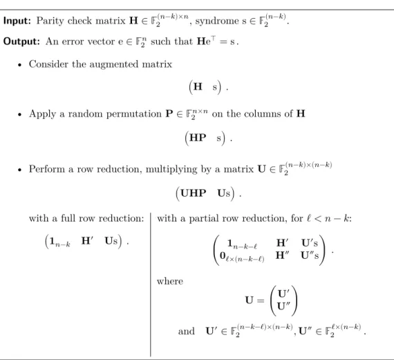
Input: Parity check matrix H ∈ 𝔽(𝑛−𝑘)×𝑛
2 , syndrome s ∈ 𝔽 (𝑛−𝑘) 2 .
Output: An error vector e ∈ 𝔽𝑛
2 such that He⊺ =s .
• Consider the augmented matrix
(H s) . • Apply a random permutation P ∈ 𝔽𝑛×𝑛
2 on the columns of H
(HP s) .
• Perform a row reduction, multiplying by a matrix U ∈ 𝔽(𝑛−𝑘)×(𝑛−𝑘) 2
(UHP Us) . with a full row reduction:
(1𝑛−𝑘 H′ Us) .
with a partial row reduction, for ℓ < 𝑛 − 𝑘: ( 1𝑛−𝑘−ℓ H ′ U′s 0ℓ×(𝑛−𝑘−ℓ) H″ U″s) . where U = (UU″′) and U′∈ 𝔽(𝑛−𝑘−ℓ)×(𝑛−𝑘) 2 ,U″∈ 𝔽 ℓ×(𝑛−𝑘) 2 .
Figure 3.2: One iteration of Information Set Decoding principle
Therefore, any of these algorithms can be used to solve either SD(𝑛, 𝑘, 𝑤) or CF(𝑛, 𝑘, 𝑤) for some parameters 𝑛, 𝑘, 𝑤. If we write one of these algorithms as 𝒜 then both problems have the same workfactor
𝒲ℱ𝒜(𝑛, 𝑘, 𝑤) .
Let us only consider the Prange algorithm to solve SD(𝑛, 𝑘, 𝑡) with 𝑡 = 𝑜(𝑛) for now. The dominating factor in the work factor for this algorithm is the average number of trials before finding an error-free information set. It is equal to (𝑛𝑡)
(𝑛−𝑘 𝑡 ) . We have 1 𝑡 log2( (𝑛𝑡) (𝑛−𝑘𝑡 )) ∼ 1 𝑡 log2( 𝑛𝑡 (𝑛 − 𝑘)𝑡) = 𝑐 with 𝑐 = − log2(1 − 𝑘 𝑛) as 𝑛 goes to infinity, using Stirling’s formula. So the work factor is 2𝑐𝑡(1+𝑜(1)).
For the other variants known at the moment of writing this document, the following result from [CS15] shows that asymptotically, when 𝑡 = 𝑜(𝑛), the work factor is the same.
Proposition 3.5. [CS15] Let 𝑘 and 𝑡 be two functions of 𝑛 such that lim𝑛→∞𝑘/𝑛 = 𝑅,
0 < 𝑅 < 1, and lim𝑛→∞𝑡/𝑛 = 0. For any algorithm 𝒜 among the variants of [Pra62; Ste88;Dum91;BJMM12;MMT11;MO15], we have
𝒲ℱ𝒜(𝑛, 𝑘, 𝑡) = 2𝑐𝑡(1+𝑜(1)), 𝑐 = −log2(1 − 𝑅)
3.3. Best known attacks on underlying hard problems 23 The quasi-cyclic structure of a code means that any blockwise circular shift of a codeword is also a codeword and that, given an error pattern, any circular shift of its syndrome corresponds to a blockwise circular shift of the same error pattern. It has been shown in [Sen11] that one can exploit this structure and expect a polynomial gain in the work factor of an ISD algorithm. In practice the work factor for finding low weight codeword in the dual is divided by (𝑛 − 𝑘) and the work factor for decoding is divided by √
𝑛 − 𝑘.
So, the work factor to solve the quasi-cyclic SD(𝑛, 𝑘, 𝑡) problem is 𝒲ℱQCSD(𝑛, 𝑘, 𝑡) ∶= 𝒲ℱ√𝒜(𝑛, 𝑘, 𝑡)
𝑛 − 𝑘 = 2
𝑐[1/2+𝑡(1+𝑜(1))]−log2(𝑛)/2
and to solve the quasi-cyclic CF(𝑛, 𝑘, 𝑤) problem is 𝒲ℱQCCF(𝑛, 𝑘, 𝑤) ∶= 𝒲ℱ𝒜(𝑛, 𝑘, 𝑤)
𝑛 − 𝑘 = 2
Chapter 4
BIKE
[BIKE] uses QC-MPDC codes in a Niederreiter cryptosystem. Its characteristics are particularly relevant to the NIST Post Quantum Cryptography standardization process1.
It has (i) small keys, and (ii) efficient, low-complexity algorithms. It is therefore suitable for both software and hardware implementations. The former category received optimization attention using the specialized instructions of modern x86 processors, see [DG19;DGK20a]. The latter has also been studied for microcontrollers, see [HMG13;MG14], as well as Field-Programmable Gate Array (FPGA), see [HMG13;MOG15b;HC17;HWCW19;RMG20]. In these works, improvements or tradeoffs are obtained by focusing on the polynomial multiplication needed for encapsulation and decapsulation, and on the polynomial inversion for the key generation.
Table 4.1: BIKE parameters.
𝜆 𝑤 𝑡 𝑟CPA 𝑟CCA ℓ
128 142 134 10 163 12 323 256 192 206 199 19 853 24 659 256 256 274 264 32 749 40 973 256 Let us fix the following parameters:
• 𝑟: the block size of a parity check matrix, • 𝑛 = 2𝑟: the length of a code,
• 𝑑: the column weight of a parity check matrix, • 𝑤 = 2𝑑: the row weight of a parity check matrix, • 𝑡: the weight of an error pattern,
• ℓ: the message space size,
• 𝜆: the security parameter, in bits. We define the following sets:
• ℛ𝑟≃ 𝔽2[𝑥]/(𝑥𝑟− 1): the set of 𝑟 × 𝑟 circulant matrices,
• ℛ𝑟,𝑑: the set of 𝑟 × 𝑟 circulant matrices of row weight 𝑑,
• ℰ𝑛,𝑡: the set of vectors of 𝔽2𝑛 with Hamming weight 𝑡.
26 Chapter 4. BIKE
Table 4.2: BIKE specification.
• KeyGen(seed) ∶= { (h 0,h1) $ ← ℛ𝑟,𝑑; h ← h1h−10 ; 𝜎← {0, 1}$ ℓ; return(h0,h1, 𝜎),h; }, • Encaps(h) ∶= { m $ ← {0, 1}ℓ; (e0,e1) ←H(𝑚); c ← (e0+e1h, m ⊕ L(e0,e1)); 𝐾 ←K(m, c); return𝐾,c; }, • Decaps((h0,h1, 𝜎),c) ∶= { e′←Decode⟂MDPC(c0h0,h0,h1); m′←c 1⊕L(e′); ife′≠H(m′)then return K(𝜎, c); otherwise return K(m′,c); }.
Where H, K and L are three hash functions. H has outputs in ℰ𝑛,𝑡, K and L in {0, 1}ℓ.
BIKE is defined2 in Table4.2.
This entire document is devoted to the decoder, so we will not detail its operation in this preliminary chapter. We will however explain the conversion used and what it implies for security, in particular the necessary conditions imposed on the decoder. We will also detail why the block size should be chosen carefully.
4.1 Security
Using notations from §3.2we can build PKE0= (KeyGen0,Encrypt0,Decrypt0), a
Nieder-reiter cryptosystem using QC-MDPC codes by taking • CodeGen⟂(seed) ∶= { H0 $ ← ℛ𝑟,𝑑; H1 $ ← ℛ𝑟,𝑑; H ← (1𝑟 H−10 H1); return(H, H0); }, • Decode⟂(H, H 0,s) ∶= { s′←H0s; returnDecode⟂ MDPC((H0 H0H), s′); }.
with 𝒦pub= ℛ2𝑟, 𝒦priv= ℛ𝑟,𝑑, ℳ = ℰ𝑛,𝑡, 𝒞 = 𝔽2𝑟.
However, applying Niederreiter construction directly in this PKE is not secure. Indeed, the problem is to leave the complete control of the error pattern to the person who encrypts. In the hand of a malicious adversary, this could be used in a reaction attack such as [GJS16] where particular error patterns allow them to gather information about the private key.
Even outside practical concerns, this issue is already taken into account in the analysis of [HHK17]. Indeed, if we want to use the Theorem 2.5 to prove that the scheme is IND-CCA secure, we need to make sure that the PKE is 𝛿-correct with 𝛿 really small. Definition2.4of 𝛿-correctness concerns the maximum probability of failure on all possible
1https://csrc.nist.gov/projects/post-quantum-cryptography 2The notation $
←means drawing uniformly at random from the right side and assign it to the left side using seed.
4.1. Security 27 messages, and it is difficult to prove that no message will be decoded with less success than the average. It is in fact not true, the question of particular problematic error patterns will be discussed in Chapter16on the phenomenon known as the “error floor”.
To circumvent this problem, BIKE adds randomization to the error pattern. Instead of choosing a random message m and using it directly as an error pattern to compute the syndrome, the message m is first hashed and the hash H(m) is used as the error pattern. The soundness of such a process is guaranteed by a commitment: m ⊕ L(H(m)).
Using the more compact polynomial representation, we obtain the specification in Table4.2.
To apply Theorem2.5, we have to study the IND-CPA security of the scheme first. It relies on the quasi-cyclic versions of the problems SD(𝑛, 𝑘, 𝑡) and CF(𝑛, 𝑘, 𝑤). We define the function:
• QCSD𝑟,𝑡((e0,e1) ,h, s) for e0,e1,h, s ∈ 𝔽2[𝑥]/(𝑥𝑟− 1).
It returns 1 if ∣e0∣ + ∣e1∣ = 𝑡 and e0+e1h = s, and 0 otherwise.
For any probabilistic polynomial time algorithm 𝒜 taking for inputs h ∈ 𝔽2[𝑥]/(𝑥𝑟− 1)
and s ∈ 𝔽2[𝑥]/(𝑥𝑟− 1), and producing as output an element of (𝔽2[𝑥]/(𝑥𝑟− 1)) 2
, we define its advantage concerning the one-wayness of the cipher as:
AdvOWQCSD𝑟,𝑡(𝒜) =Pr [ QCSD𝑟,𝑡(𝒜(h, e0+e1h), h, e0+e1h) ∣ h ∈ ℛ𝑟, (e0,e1) ∈ ℰ𝑛,𝑡] .
For any probabilistic polynomial time algorithm 𝒟 taking as input h ∈ 𝔽2[𝑥]/(𝑥𝑟− 1) ,
and producing 0 or 1 as output, we define its advantage concerning the distinguishability of the parity check matrix as:
AdvIND
QCCF𝑟,𝑤(𝒟) = ∣Pr [𝒟 (h1h
−1
0 ) = 1 ∣h0,h1∈ ℛ𝑟,𝑤/2] −Pr [𝒟 (h) = 1 ∣ h ∈ ℛ𝑟]∣ .
Theorem 4.1. [BIKE, §C.1.2] For any IND-CPA adversary 𝒜 against PKE1 there exists
an adversary 𝒜′ against QCSD
𝑟,𝑡 and a distinghuer 𝒟 against QCCF𝑟,𝑤 running in about
the same time as 𝒜 such that
AdvIND−CPAPKE1 (𝒜) ≤
1 2Adv OW QCSD𝑟,𝑡(𝒜 ′) +1 2Adv IND QCCF𝑟,𝑤(𝒟) .
The number of bits of security of a problem is usually defined as the smallest 𝜆 such that for any adversaries 𝒜
Time(𝒜) Adv(𝒜) ≥ 2𝜆
where Time(𝒜) is the running time of 𝒜. Note that if 𝒜 makes 𝑞 queries to any oracle then Time(𝒜) > 𝑞.
To summarize Theorem2.5& Theorem4.1, in order to have 𝜆 bits of security against an IND-CCA adversary we want:
• 𝒲ℱQCSD(2𝑟, 𝑟, 𝑡) > 2𝜆,
• 𝒲ℱQCCF(2𝑟, 𝑟, 𝑤) > 2𝜆,
• 2ℓ> 2𝜆,
• 𝛿 < 2−𝜆 i.e. DFR(decoder) < 2−𝜆.
Remember that we call DFR the decoding failure rate of a decoding algorithm. The best known algorithm to solve the underlying problems are variants of the ISD algorithms
28 Chapter 4. BIKE
that we discussed in §3.3. So to satisfy the first two points we should have, in a first approximation:
21/2+𝑡(1+𝑜(1))−log2(𝑛)/2> 2𝜆 and 21+𝑤(1+𝑜(1))−log2(𝑛)> 2𝜆
for some security parameter 𝜆. Parameters should nevertheless be determined by consider-ing the actual work factors of ISD algorithms.
If only the first three points are verified, the system is still IND-CPA secure. The last point is the main concern of this document and grants IND-CCA security if verified.
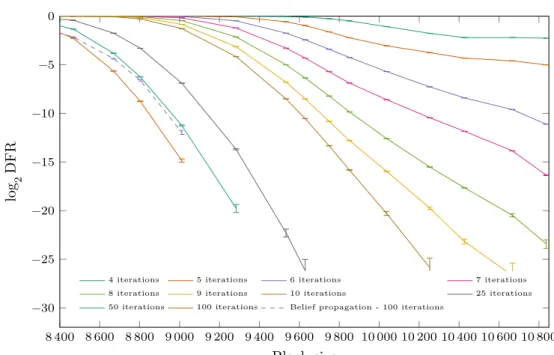
Table4.1 gives the sets of parameters of [BIKE]. Two values for the block size 𝑟 are provided, 𝑟CPA that verifies the first three conditions and 𝑟CCAthat was the value retained
in [BIKE] to have a DFR low enough for IND-CCA security using the method that we detail in Chapter14.
4.2 Block size
Squaring. If the block size 𝑟 is an even number, it has been shown in [Lön+16] that an attacker can decrease the cost of the ISD attacks using a squaring technique.
Remember that we are in the context of Proposition 1.31 and we are dealing with polynomials in 𝔽2[𝑥]/(𝑥𝑟− 1). While, in [Lön+16], only a McEliece variant using
QC-MDPC is mentioned, it can easily be translated for the Niederreiter variant and this is what we will do here.
As we are dealing with a field of characteristic 2, squaring a polynomial
𝑟−1 ∑ 𝑖=0 𝑎𝑖𝑥𝑖 gives, if 𝑟 is even, 𝑟−1 ∑ 𝑖=0 𝑎𝑖𝑥2𝑖= 𝑟/2−1 ∑ 𝑖=0 (𝑎𝑖+ 𝑎𝑖+𝑟/2)𝑥2𝑖 mod (𝑥𝑟− 1) . (4.1)
Attacks on the system can be roughly described, for a private keyh∈ 𝔽2[𝑥]/(𝑥𝑟− 1)
and a syndrome s∈ 𝔽2[𝑥]/(𝑥𝑟− 1), as follows.
Key recovery Message recovery Findh0,h1∈ 𝔽2[𝑥]/(𝑥𝑟− 1)such that
∣h0∣ ≤ 𝑤
∣h1∣ ≤ 𝑤
andh0h=h1
Finde0,e1∈ 𝔽2[𝑥]/(𝑥𝑟− 1)such that
∣e0∣ + ∣e1∣ ≤ 𝑡
ande0+e1h=s
If we now square all equations, we obtain the following. Note that a squared polynomial has no monomial of odd degree, hence the dimension of the problem is divided by 2.
Key recovery (squared) Message recovery (squared) Findh2 0,h21∈ 𝔽2[𝑥]/(𝑥𝑟− 1)such that ∣h2 0∣ ≤ 𝑤2 ∣h2 1∣ ≤ 𝑤2 andh2 0h2=h21 Finde2 0,e21∈ 𝔽2[𝑥]/(𝑥𝑟− 1)such that ∣e2 0∣ + ∣e21∣ ≤ 𝑡2 ande2 0+e21h2=s2
4.2. Block size 29 Now the weights 𝑤2and 𝑡2 are not specified. In (4.1), we say that there is a collision if
there exists an 𝑖 such that
𝑎𝑖= 𝑎𝑖+𝑟/2= 1 .
Each collision decreases the weight of the squared polynomial by 2 compared to the original polynomial. So the squared versions of the problems are simpler (remember from §3.3that the complexity of the problems depends mainly on 𝑡 and 𝑤).
Of course, the process can be repeated as many times as the dyadic valuation of 𝑟. And each time the process is applied, since the dimension is divided by two, the probability of having a collision increases and therefore the weights3 𝑤
2𝑖 and 𝑡2𝑖 decrease as well.
Square roots. Once a solution to the squared problem is found, it remains to lift it to
return to the original problem. Say a′2= ∑𝑟/2−1 𝑖=0 𝑖even
𝑎′
𝑖𝑥2𝑖is a solution to a problem. For any
position 𝑖 such that 𝑎′
𝑖 = 1then
𝑎′
𝑖= 𝑎𝑖+ 𝑎𝑖+𝑟/2= 1
so either 𝑎𝑖= 1or 𝑎𝑖+𝑟/2= 1.
A solution to the initial problem is found using an ISD algorithm with the additional leverage provided by this information. To be more precise, if we remember the general structure of such an algorihm explained in Figure 3.2, rather than applying a random permutation P to the matrix, we restrict ourselves to permutations that do not place the above-mentioned positions in the information set. In other words, these positions will always be permuted to the first 𝑛 − 𝑘 (or 𝑛 − 𝑘 − ℓ) positions.
Doing this is equivalent to removing 2 ⋅ 𝑤2 symbols (puncturing the code) so this
increases the code rate slightly. And from Proposition3.5we know that this will slightly increase the contribution of the factor 𝑐 in the exponent of the workfactor.
However, if many collisions occurred during the squaring process, the decrease in the weight 𝑤 (or 𝑡) makes this algorithm worthwhile from an attacker’s point of view.
As with the squaring process, this process too can be repeated as many times as the dyadic valuation of 𝑟.
To summarize, an attacker would perform squarings, then look for solution to the reduced problem, and finally lift the solution by computing square roots. The dominating factor in the complexity of this attack is the first solution to the reduced problem. It is particularly interesting for weak keys: keys with numerous collisions once squared. It has been shown in [Lön+16], for some parameters such that 24divides 𝑟, that the logarithm
of the cost of the attack divided by the probability of having a weak key is at least 10 bits below the expected security level.
Generalization. The attack was further generalized in [CT19]. This paper adopts a different point of view. It studies codes with a non-trivial automorphism group i.e. a group of isometries that leave the code globally invariant. The code is then folded: for a given codeword, we consider the sum of its images under the elements of the automorphism group. The result is the same as in the previous paragraphs, the decoding problem is reduced to a smaller dimension, a smaller error weight with the same code rate.
To do the connection with the previous paragraphs, for a quasi-cyclic code with an even block size, the permutation that, in each block, shifts the positions by 𝑟/2 coordinates is an isometry and along with the identity it forms an automorphism group.
This could be done for any non-trivial divisor 𝑟′ of 𝑟, not just 2. We would then
consider shifts in multiples of 𝑟/𝑟′, giving a group of automorphism of the order 𝑟′. To
avoid any such attack, 𝑟 must therefore be a prime number.
3Repeated squaring gives the same equations as above, we simply need to change each exponent by 2
by 2𝑖and the weights 𝑤
30 Chapter 4. BIKE
In fact, to avoid any other structural attack, in [BIKE], the block size 𝑟 is chosen so that the polynomial 𝑥𝑟− 1has only two irreducible factors:
𝑥 + 1 and 𝑥𝑟−1+ 𝑥𝑟−2+ ⋯ + 𝑥 + 1 .
Equivalently, it means that 2 is primitive modulo 𝑟 − 1.
It also ensures that any polynomial of 𝔽2[𝑥]/(𝑥𝑟− 1)with an odd Hamming weight is
invertible, thus avoiding having to integrate any rejection process in the key generation4.
4Remember that in the Niederreiter setting, the first block h
0 has to be inverted to compute the
Chapter 5
Syndrome weight and counters in
a regular MDPC code
There is a quantity that plays a fundamental role in decoding, notably for bit-flipping which is the type of algorithms used for [BIKE]1. That quantity is the counter of a position, i.e.
the number of unsatisfied parity check equations involving that position. In this chapter, we study it as a subject in its own right and explain the relation with the syndrome weight. This chapter is a review of some results of [Cha17] that we will need and refer to regularly throughout this document.
Notation. For this chapter, we consider a (𝑑, 𝑤)-regular [2𝑟, 𝑟]-MDPC code with a (sparse)
parity check matrix H and consider the problem of finding the error vector e of weight 𝑡 from the syndrome s = He⊺ with the parameters
• 𝑟: the block size of the parity check matrix; • 𝑛 = 2𝑟: the length of the code,
• 𝑑: the column weight of the parity check matrix; • 𝑤 = 2𝑑: the row weight of the parity check matrix, • 𝑡: the weight of the error pattern.
We write2 H = (h0 h1 ⋯ h𝑛−1) = ⎛ ⎜ ⎜ ⎜ ⎜ ⎜ ⎝ h⊺ 0 h⊺ 1 ⋮ h⊺ 𝑟−1 ⎞ ⎟ ⎟ ⎟ ⎟ ⎟ ⎠
where h0, … ,h𝑛−1 are the columns of H and h⊺0, … ,h⊺𝑟−1 are the rows of H.
5.1 Fundamental quantities
Definition 5.1. For any position 𝑗 ∈ {0, … , 𝑛 − 1}, we call counter, the quantity
𝜎𝑗(H, s) ∶= ∣h𝑗⋆s∣ .
1After all BIKE stands for Bit-Flipping Key Encapsulation.
2Note that for a quasi-cyclic code, in the polynomial formalism, if the parity check matrix is represented
as (h0,h1)with h0,h1∈ 𝔽2[𝑥]/(𝑥𝑟− 1)for some block size 𝑟, then we have, for 𝑖 = 0, 1
∀𝑗 ∈ {0, … , 𝑟 − 1},h𝑖⋅𝑟+𝑗= 𝑥𝑗h𝑖.