Cryptographie post-quantique : étude du décodage des codes QC-MDPC

HAL Id: hal-01664082

https://hal.inria.fr/hal-01664082

HAL is a multi-disciplinary open access

archive for the deposit and dissemination of sci-entific research documents, whether they are pub-lished or not. The documents may come from teaching and research institutions in France or abroad, or from public or private research centers.

L’archive ouverte pluridisciplinaire HAL, est destinée au dépôt et à la diffusion de documents scientifiques de niveau recherche, publiés ou non, émanant des établissements d’enseignement et de recherche français ou étrangers, des laboratoires publics ou privés.

codes QC-MDPC

Valentin Vasseur

To cite this version:

Valentin Vasseur. Cryptographie post-quantique : étude du décodage des codes QC-MDPC. Cryptog-raphy and Security [cs.CR]. 2017. �hal-01664082�

Mater Cybersecurity

Master of Science in Informatics at Grenoble

Master Informatique / Master Mathématiques & Applications

Cryptographie post-quantique : étude du

décodage des codes QC-MDPC

Valentin Vasseur

September 2017

Research project performed at Inria Paris

Under the supervision of:

Nicolas Sendrier, Inria Paris

Defended before a jury composed of:

Jean-Guillaume Dumas

Jean-Louis Roch

Nicolas Sendrier

Vanessa Vitse

Abstract

In this work, I look at a variant of the McEliece cryptosystem aiming at reducing the key size. This scheme is based on correcting codes and it relies on a simple probabilistic decoding algorithm. However the failures of the decoding algorithm can be used to retrieve the secrete key. During my internship I tried to reduce that decoding failure rate by introducing as little complexity to the algorithm as possible. Here, I present a few variants of the algorithm and look at how they perform on simulations. Finally I try to find models on the evolution of certain quantities during the algorithm. The knowledge of these evolutions could be used to improve the variants of the algorithm.

Résumé

Dans ce document, je m’intéresse à une variante du cryptosystème de McEliece visant à réduire la taille des clés. Ce système se base sur la théorie des codes correcteurs et utilise un algorithme de décodage itératif probabi-liste simple. Cependant, les échecs au décodage peuvent être utilisés pour récupérer la clé secrète. Pendant mon stage, j’ai essayé de réduire ce taux d’échec au décodage en introduisant aussi peu de compléxité que possible dans l’algorithme. Ici, je présente quelques variantes de cet algorithme et je regarde leurs comportements sur des simulations. Enfin, j’essaie de trouver des modèles sur l’évolution de certaines quantités intervenant dans l’algo-rithme. La connaissance de ces évolutions pourrait être utilisée pour amé-liorer les variantes de l’algorithme.

Contents

2.3 Decoding algorithms for the MDPC codes . . . 6

2.4 A key recovery attack using decoding failures . . . 9

3 Objectives 10 4 State of the art 11 4.1 Algorithm originally proposed . . . 11

4.2 Improvements using the syndrome weight . . . 12

5 Decoding QC-MDPC codes 18 5.1 Empirical improvements . . . 18

5.2 Theoretical analysis . . . 23

6 Conclusion 36

In this document, we will focus on the syndrome decoding problem: given H ∈ Fp2×n

and s∈ Fp₂we want to find e ∈ Fn

2 such that He⊤ = s. We will use the following way of

representing the different objects involved.

H hi

h⊤_j

e

s

We will use the variable i to index a row of the matrix H and the variable j a column. B(n, p) The binomial distribution with parameters n and p

d Hamming weight of a column

e An error vector

G A generator matrix

H A parity matrix

hi The i-th row of the parity check matrix H

h⊤_j The j-th colum of the parity check matrix H

n Length of the code (in this document we always have n = n0· p)

CONTENTS iv

p Dimension of the code

s A syndrome

w Hamming weight of a row Proposed parameters in [MTSB13]: Security n0 p d t 80 2 4, 801 45 84 80 3 3, 593 51 53 80 4 3, 079 55 42 128 2 9, 857 71 134 128 3 7, 433 81 85 128 4 6, 803 85 68 256 2 32, 771 137 264 256 3 22, 531 155 167 256 4 20, 483 161 137

Context

Most of the cryptosystems used nowadays rely on problems such as the integer fac-torisation or the discrete logarithm. Those problems could be solved in a polynomial time with a sufficiently powerful quantum computer using Shor’s algorithm [Sho97] or a variant [PZ03].

Even if the current state of quantum computing does not allow an attacker to break widespread algorithms such as RSA, DH, ECDH or ECDSA, the threat is real if we want long term secrecy. In response to that possible threat, the NIST1_{will start a process to}

standardise quantum-resistant cryptographic algorithms (or post-quantum algorithms) in November 2017.

In this document, I will present a post-quantum cryptosystem using error correcting codes (also known as code-based cryptography), a variant of the McEliece cryptosys-tem [McE78] which uses QC-MDPC codes [MTSB13]. I will specifically focus on the decoding algorithm of those codes for which there are security concerns [GJS16].

2

Preliminaries

We are interested in decoding a type of linear error correcting code used in a variant of the McEliece cryptosystem. In this chapter we shall therefore recall the definitions and main results about those objects.

2.1 McEliece cryptosystem

Definition 2.1. An [n, k]-linear codeC is a linear subspace of Fn

q of dimension k.

We say that such a code is of length n and dimension k. If q = 2 we say thatC is a

binary code.

The vectors ofC are called codewords.

Definition 2.2. A generator matrix G of a codeC ⊂ Fn

q is a matrix whose rows form a

basis of the linear subspaceC. Any vector v ∈ Fk

qcan be mapped to a codeword c∈ C with:

c = vG .

We say that we encode the message v as the codeword c.

A parity check H matrix is a matrix such that c∈ C if and only if Hc⊤ = 0. For any vector y ∈ Fn

q, the vector Hy⊤is called the syndrome of y.

Definition 2.3. The Hamming weight of a vector v ∈ Fn

q is the number of its non-zero

components:

wt(v) =|{i | vi ̸= 0}| .

The Hamming distance between two vectors v, w ∈ Fn

q is the Hamming weight of

their difference:

d(v, w) = wt(w− v) = |{i | vi ̸= wi}| .

The minimum distance of a code C is the minimum distance between two distinct codewords:

∆(C) = min

c1,c2∈C

c1̸=c2

Intuitively, correcting codes add redundancy in a message so that the noise which is added during transmission can be removed. A noisy codeword will be at a certain distance of a codeword. If that distance is small enough, we can find the codeword which hopefully corresponds to the transmited message.

Definition 2.4. LetC be an [n, k]-linear code of miminum distance d, c ∈ C be a

code-word and e∈ Fn

q be an error pattern of weight less than d−1

2 . We write v = c + e.

We say that we decode the message v if we find c∈ C knowing v.

If the codeC has a minimum distance of d, we can detect up to d − 1 errors and, in theory, correct up to⌊d−1

2

⌋

errors.

In practice, for the decoding process to be fast, we add a structure to the codeC. For example, Reed-Solomon codes are based on polynomials over finite fields and decod-ing can be achieved usdecod-ing a variant of the extended Euclidean algorithm (among other algorithms).

In this document we will talk about MDPC1_{codes which are derived from the LDPC}2

codes. They both use a probabilistic decoding algorithm which requires a sparse parity check matrix.

Definition 2.5. The McEliece cryptosystem uses the family of the Goppa codes3_{. The}

main idea behind the system is that we can give a way to encode a mesage (the public key ˆ

G) without revealing the decoder (the private key (S, G, P )).

C ← Goppa(n, k, t) G generator matrix forC

S random k× k invertible matrix

P random n× n permutation matrix m∈ {0, 1} k c′ = m ˆG e← {0, 1}n |e| = t ˆ c = c′P−1 ˆ m =Decode(ˆc) m = ˆmS−1 ˆ G = SGP c = c′+ e

Here we denote by Goppa(n, k, t) the family of Goppa codes of length n, dimension

kand capable of correcting t errors.

The security of the McEliece cryptosystem relies on the difficulty of decoding a ran-dom linear code. The best algorithms to solve this problem are all variations of the Prange algorithm [Pra62].

1. Moderate Density Parity Check 2. Low Density Parity Check

CHAPTER 2. PRELIMINARIES 4

2.2

MDPC-McEliece

Goppa codes are interesting in such a scheme because they provide a high error cor-rection capacity and they have a parity check matrix which is hardly distinguishable from a random matrix. But their main issue is the key size which prevents some lightweight or embedded usages. In [Aug+15], the proposed parameters for 128 bits of post-quantum security for the McEliece cryptosystem are n = 6, 960, k = 5, 413, t = 119, this gives a public key size of k× (n − k) = 8, 373, 911 bits.

Definition 2.6. As their names suggest, LDPC4_{and MDPC}5 _{codes have respectively}

a parity check matrix of low and moderate density. Here the density of the matrix is defined by the weight of its rows.

For LDPC, rows have a constant weight (usually less than 10). For MDPC they have a weight which scales in O(√n)where n is the length of the code.

LDPC codes are widely used in telecommunications. A cryptographic scheme has been proposed using LDPC codes [BCGM07] in a McEliece variant where they replace the Goppa codes. However a weakness was later found [BC07] which could break the system. The proposed fix used matrices with a specific structure which has been broken in [OTD10]. Finally in [BBC08] a more general structure was proposed fixing these is-sues. As in the McEliece cryptosystem, (S, G, P ) would be the private key, and the pub-lic key would be ˆG = SGP with G the generator matrix of an LDPC code. In [BBC08],

P has to be an invertible matrix of moderate weight.

In [MTSB13], authors took a different approach. They directly generate a parity check matrix of moderate density. Such a modification circumvents all the previous at-tacks on the LDPC-McEliece system. This generates codes with a worse decoding cap-ability but it is still good enough to use the usual decoding algorithms. Note that this system does not require the matrices P and S as in the original McEliece system.

Definition 2.7. The MDPC-McEliece cryptosystem works as follows.

H random k×n matrix with rows of weight w G = (Ik| ˜G)a generator matrix corresponding to H m∈ {0, 1}n−k c′ = mG e← {0, 1}n |e| = t m =Decode(ˆc) G c = c′+ e

4. Low Density Parity Check 5. Moderate Density Parity Check

As for the original McEliece system, for 128 bits of post-quantum security, MDPC-McEliece would require huge key size. But it becomes interesting if we use a quasi-cyclic version of the MDPC codes.

Definition 2.8. A circulant matrix is a matrix such that it is uniquely determined by its

first row. Indeed each row is the cyclic permutation with an offset of one of the row just

above it. _       m0 m1 · · · mn−1 mn mn m0 m1 · · · mn−1 . .. ... . .. m2 · · · mn m0 m1 m1 m2 · · · mn m0       

The set of circulant matrices of size n×n over a field K is isomorphic to K[X]/(Xn₋

1).

Definition 2.9. A QC-MDPC6_{code is a code whose parity check matrix H consists in}

n0 blocks which are p× p circulant matrices where p is a prime number. Those blocks

have the same row weight and column weight d. The row weight of the parity check matrix is therefore w = n0d. H =                 · · · H0 Hn0

As for circulant matrices, quasi-cyclic matrices are entirely described by their first row. For the QC-MDPC-McEliece cryptosystem, this yields public keys of size 32, 771 bits for 128 bits of post-quantum security.

The security of the system relies on the two following problems: — decoding t errors in a quasi-cyclic [n, n− p] linear code;

— deciding whether the code spanned by some block circulant p× n matrices has a minimum distance less than w.

Both problems are NP-hard in the non quasi-cyclic case. They are conjectured hard in the quasi-cyclic case and we can choose the parameters n, p, w, t such that it takes at least 2κ_{operations to solve them for κ-bit security.}

CHAPTER 2. PRELIMINARIES 6

2.3

Decoding algorithms for the MDPC codes

Decoding from a random linear code is usually hard. For MDPC (or LDPC), there are efficient algorithms, they use the fact that the parity check matrix is sparse.

Those decoders can be split into two categories:

— hard decision algorithms: they operate on data consisting of 0 and 1; — soft decision algorithms: they can use all the values in-between.

Soft decision algorithms have better correction capabilities but are more complex to implement. Hard decision algorithms are better suited for an embedded implementation at the expense of the correction capability.

In the next following sections, we will detail a hard decision algorithm — the bitflip-ping algorithm — and a soft decision algorithm — the belief propagation algorithm.

For convenience, we will sometimes consider a vector v∈ Fn

2 as the set of indices of

its nonzero values:

v ={i ∈ {1, . . . , n} | vi ̸= 0} .

We will frequently need to use the cardinality of the intersection of two vectors. For this, we will use different equivalent points of view:

|h ∩ v| = ⟨h, v⟩Z =

∑

k

hkvk.

We will call

— m the transmitted message,

— c = mG the corresponding codeword, — e the error pattern,

— y the received noisy codeword (y = c⊕ e).

We recall that the syndrome s = Hy⊤ is zero if and only if y is a codeword. So we have

s = Hy⊤ = Hc⊤⊕ He⊤= He⊤=⊕

j∈e

h⊤_j .

We will say that the elements in e are erroneous positions or errors. The goal of the decoding process is finding the vector e.

For any i∈ {1, . . . , p} we say that the i-th equation is satisfied if |hi∩ y| (or

equival-ently|hi∩ e|) is even and unsatisfied if it is odd. The equation can be written as: n

∑

i=0

hjiei = 0 mod 2 .

We have achieved the decoding process when we have a vector y such that its syndrome is zero i.e. when all the equations are satisfied.

2.3.1

Bit flipping

The bitflipping algorithm was first proposed by Gallager in [Gal63] to decode LDPC codes. It relies on the fact that each bit of the syndrome tells us if the corresponding equation is satisfied or not. Thus if a position is involved in many unsatisfied equations, it is probably an error.

The algorithm relies on the computation, for each position j, of a counter with the formula σj = ⟨h⊤j, s⟩Z. This counter is the number of unsatisfied equations involving

the position j.

The algorithm is iterative and on each iteration it will compute all the σj values and

flip the positions for which the counter is over a certain threshold. When we have flipped all the errors, y is a codeword and so its syndrome is zero.

Algorithm 1 The bitflipping algorithm

procedure Bitflipping(y, H) ▷ y = (y1, . . . , yn)∈ {0, 1}n while Hy⊺ ̸= 0 do ▷ H = (h1, . . . , hn)∈ {0, 1}k×n s← Hy⊺ for j = 1, . . . , n do if σj =⟨s, h⊤j ⟩Z≥ threshold then yj ← 1 − yj return y

It is really simple but the hard part is choosing a threshold. In the LDPC case, the column weight is as big as a few units but for MDPC it can be as big as 161 and a bad choice of threshold can make the decoding process fail (this will further be discussed in chapter 4).

In the case of MDPC, decoding is usually achieved in less than ten iterations.

2.3.2 Belief propagation

In [Gal63], the author describes another algorithm which he calls “probabilistic de-coding”, it is now more commonly referred to as a belief propagation algorithm or sum-product algorithm.

The basic idea behind this algorithm is that we want to get a good estimation of the probabilities P (cj = 1 | y) and P (cj = 0 | y) where y is the received vector (a noisy

codeword) and c is the sent codeword. The estimation of these probabilities is made iteratively.

First we compute the conditional probabilities for the each equation to be satisfied or not knowing the components of y affected by this equation. Then we compute the con-ditional probabilities for the components of y knowing the probabilities of the equations they are involved in. We then iterate the process. This can be seen as a probability tree.

CHAPTER 2. PRELIMINARIES 8 ... ... ... ... ... ... ... ... ... ... ... ... ... ... ... ... ... ... ... ... ... ... ... ... ... ... ... ... ... ... ... ... ... ... ... ... root root equations tier 1 tier 1 equations

Here we have represented by a circle the positions of the vector to decode and by a square the parity check equations. This tree corresponds to a parity check matrix where every row and every column have a fixed weight of four.

Given this tree where the root is j, we will call T_j(I)the subtree going up to the I-th tier.

We will assume that the values c1, . . . , cnare all independent and that the tree has no

loop.

In our case, we know P (cj = 0| T

(0)

j )and P (cj = 1| T

(0)

j )from the parameters of

the cryptosystem, they are respectively equal to n−t n and t n. To compute P (cj = 0 | T (I+1) j )and P (cj = 1 | T (I+1) j )when I ≥ 0, we proceed

iteratively and each iteration consists in two steps that we will have to repeat for all the positions j. First step.                          P ( sicj = 0, T (I+1) j ) = ∑ {cj′|j′∈hi\{j}} P (si|cj = 0,{cj′ | j′ ∈ hi\ {j}}) ∏ j′∈hi\{j} P ( cj′T (I) j′ ) P ( sicj = 1, Tj(I+1) ) = ∑ {cj′|j′∈hi\{j}} P (si|cj = 1,{cj′ | j′ ∈ hi\ {j}}) ∏ j′∈hi\{j} P ( cj′T (I) j′ )

Second step.            P ( cj = 0T (I+1) j ) = K· P (cj = 0) ∏ i′∈h⊤_j\{i} P ( si′cj = 0, T (I+1) j′ ) P ( cj = 1T (I+1) j ) = K· P (cj = 1) ∏ i′∈h⊤_j\{i} P ( si′cj = 1, T (I+1) j′ )

It is not necessary to compute the factor K explicitely, we can use the fact that

P ( cj = 1T (I+1) j ) + P ( cj = 0T (I+1) j ) = 1 .

The algorithm will first compute the probabilities concerning the equations which will then be used to compute probabilites concerning the positions. This is called a

mes-sage passing algorithm.

Details on how to these computations can be done in practice are given in [Mac99]. Since we are computing probabilities, this algorithm requires the use of floating-point or fixed-point values. It usually needs many iterations to achieve decoding.

2.4 A key recovery attack using decoding failures

In [GJS16], the authors describe a way to recover the private key in the QC-MDPC scheme.

They call spectrum the set of all the existing distances between two ones in a vector. The decoding algorithm will have a slightly smaller probability to fail when the error vector’s spectrum and the private key’s spectrum have a nonempty intersection. Thus if we provide enough generated messages to a decoder which signals decoding failures, we are able to recover the private key’s spectrum by looking at the distances in the error vectors triggering the least failures.

Then they provide a reconstruction algorithm to recover the private key from the spectrum.

Authors compare two cases: the CPA case where the attacker can build the error vector and the CCA case where the error vector is truly random. They claim that full recovery of the key can be done in 240 million calls to the decoder for the CPA case and 356 million for the CCA case using the 80-bit security parameters.

In this attack, the decoding algorithm used by the authors has the same fixed threshold for all the iterations. In [MTSB13], better approaches were suggested knowing that using a fixed threshold does not give the best error-decoding capability.

3

Objectives

The main goal of my internship at Inria Paris was improving the bitflipping algorithm used with QC-MDPC codes.

The need for an improvement in the decoding algorithm comes from the fact that it currently fails with a small probability.

This probability can actually be measured if we run many simulations. If we want to use this scheme it is important to limit those failures. It is also important to have a better understanding of the way it works if we want to implement it efficiently.

Also, in response to the attack using the decoding failures, an obvious countermeas-ure would be diminishing the failcountermeas-ures until the attack is not practical.

During my internship I first tried to get a better understanding of the different de-coding algorithms for MDPC and LDPC codes by searching and understanding the work already done on them. I tried to introduce some ideas coming from the soft decoding al-gorithms into the bitflipping algorithm. I then implemented them and ran simulations to see how much of an improvement could be expected from each technique.

Finally I tried to have a more theoretical point of view in order to understand where the improvements come from.

State of the art

If we look at variants of the bitflipping algorithm for LDPC codes, it is often pro-posed to flip all the positions reaching the maximum counter value. For LDPC codes, the counters range over a small interval (typically [0; 3]) but for MDPC codes that inter-val is bigger. Such a choice would thus require many iterations since not many positions would be flipped per iteration.

4.1 Algorithm originally proposed

In the original paper [MTSB13], the proposed algorithm suggests subtracting a small value ∆ (usually ∆ = 5) to the maximum counter value and taking that value as the threshold.

In [Cho16] the choice of thresholds was made by a fixed table giving a good threshold value on average for each iteration step.

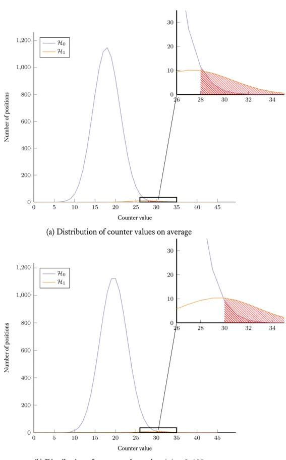
Both techniques are not always satisfying. In figure 4.1a, the distributions of the coun-ters are shown in different color depending on the fact that they correspond to erroneous positions (H1) or not (H0). A good choice for the threshold is the one corresponding to

the red dashed area: it maximises the difference between the number of errors removed and the number of errors added.

If we choose the algorithm from [MTSB13], with a non negligible probability, the maximum counter value will not give the best threshold. If that maximum is too high the choice for the threshold will be high as well. We might do an iteration in which we just flip a few errors hence not being as efficient as we could be. On the other hand if the maximum is too low we will be under the good threshold and it will flip many goood positions thus adding many errors. If we add too many errors we might get a decoding failure.

A first improvement would be using what was proposed in [Cho16]: choose the best threshold for each iteration based on an average value determined with a lot of simula-tions.

CHAPTER 4. STATE OF THE ART 12

In figure 4.1a we have the average distribution for the counter values. In figure 4.1b we have the average distribution for the counter values when then syndrome weight is higher than its average value (in this case|s| = 2, 100). Compared to the other distributions we can see that everything is shifted to the right. Thus in this case the good threshold based on the average distribution (28) will be too low and will probably lead to a failure.

The next section presents the works from [Cha17], in which the influence of the syn-drome weight on those distributions was determined. It allowed a great improvement in the decoding failure rate of the algorithm.

4.2

Improvements using the syndrome weight

Chaulet showed that the distribution of the counters can be well approximated by random variables following binomial distributions. The probabilities involved have been conditioned by the syndrome weight to give a more precise approximation and it has been used to choose better threshold values.

We will use the following values to get a better estimation of the distributions for a specific iteration.

Definition 4.1. We call Elthe number of equations affected by exactly l errors. It is the

number of rows for which the intersection with the vector e has a cardinal of exactly l.

El=|{i ∈ {1, . . . , p} | |hi∩ e| = l}|

Definition 4.2. For a position j, we define σjas the counter value of j that is:

σj =|h⊤j ∩ s| = |{i ∈ {1, . . . , p}|j ∈ hi,|hi∩ e| is odd}| .

Definition 4.3. For a position j, we writeH0the event{j ̸∈ e} and H1the event{j ∈

e}.

We can see σj as a random variable for which the distribution differs whether we are

under hypothesisH0orH1. Experimentally the following assumption can be made.

Proposition 4.4. Under hypothesisH0:

σj ∼ B(d, p0) .

Under hypothesisH1:

σj ∼ B(d, p1) .

Where B indicates the binomial distribution. The value of a counter can be seen as repeat-ing d times the independent identically distributed Bernoulli trials consistrepeat-ing in determinrepeat-ing if |{hi∩ e}| is odd for all i ∈ h⊤j.

Proposition 4.5. In proposition 4.4, we can take: p0 = P (|{hi∩ e}|is odd|H0) = t ∑ l=0 lodd (_w−1 l )(_n−w t−l ) (_n−1 t ) ; p1 = P (|{hi∩ e}|is odd|H1) = t ∑ l=0 leven (_w−1 l )(_n−w t−1−l ) (_n−1 t−1 ) .

This proposition supposes that the error vector is randomly taken out of the vectors of length n and weight t.

The next proposition allows a better knowledge of the values Elfor all l, which we

will use to give better estimates for the probabilities p0and p1on a specific instance.

Proposition 4.6. We have the following equations involving El: w ∑ l=0 El= p ; (4.1) w ∑ l=0 lodd El=|s| ; (4.2) n ∑ j=1 σj = w|s| ; (4.3) ∑ j∈e σj = w ∑ l=0 lodd lEl; (4.4) ∑ j∈e σj =|s| + w ∑ l=0 lodd (l− 1)El; (4.5) ∑ j̸∈e σj = (w− 1)|s| − w ∑ l=0 lodd (l− 1)El. (4.6) (4.7)

Proof. For any row i∈ {1, . . . , p}, |hi∩ e| is unique. This implies (4.1).

For any i∈ {1, . . . , p}, si = 1if and only if|hi∩ e| is odd, implying (4.2).

We can prove (4.3) by using the definition of σj. We will use the fact that for any i

CHAPTER 4. STATE OF THE ART 14 i, j, 1hi(j) = 1h⊤_j(i). n ∑ j=1 σj = n ∑ j=1 |h⊤ j ∩ s| = n ∑ j=1 p ∑ i=1 1_h⊤ j∩s(i) = n ∑ j=1 p ∑ i=1 1_h⊤ j(i)1s(i) = n ∑ j=1 p ∑ i=1 1hi(j)1s(i) = p ∑ i=1 1s(i) ( _n ∑ j=1 1hi(j) ) .

We can then use the fact that each row of H has a fixed weight. Similarly we can prove (4.4):

∑ j∈e σj = ∑ j∈e |h⊤ j ∩ s| = n ∑ j=1 p ∑ i=1 1_h⊤ j∩s(i)1e(j) = n ∑ j=1 p ∑ i=1 1_h⊤ j(i)1s(i)1e(j) = n ∑ j=1 p ∑ i=1 1hi∩e(j)1s(i) = p ∑ i=1 iodd n ∑ j=1 1hi∩e(j) = p ∑ i=1 iodd lEl.

The remaining formulas are clearly implied by the others.

During the decoding, for each iteration, we need to recompute the syndrome to check if the decoding is done. Its weight can be used to condition the probabilities involved in the distributions of the counters. To do so, we use the results of proposition 4.6.

Proposition 4.7. In proposition 4.4, we can take:

p0 = P (|{hi∩ e}|is odd|H0,|s|) = 1 d(n− t)   (w − 1)|s| − w ∑ l=0 lodd (l− 1)El    ; p1 = P (|{hi∩ e}|is odd|H1,|s|) = 1 dt   |s| + w ∑ l=0 lodd (l− 1)El    .

In the bitflipping algorithm, the goal is to flip as many erroneous position and as little good positions given a counter value. To express this in terms of probabilities, we want to find a threshold T such that

Using the Bayes’ theorem this becomes

P (σj ≥ T |j ∈ e)P (j ∈ e) > P (σj ≥ T |j ̸∈ e)P (j ̸∈ e) .

And if we use the fact that we have binomial distributions this becomes ( p1 p0 1− p0 1− p1 )T > n− t t ( 1− p0 1− p1 )d .

A good threshold can therefore easily be found as long as we can estimate t, p0and p1.

The first value can be estimated by using the fact that the number of errors is correl-ated to the syndrome weight.

The other two involve the value t, the syndrome weight|s| which we can compute and the value∑wl=0

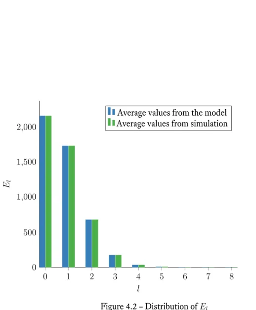
lodd(l − 1)El. The values of El becomes really small for l ≥ 4 (see

figure 4.2). So far, a choice has been made to use an average value in the computation since the values do not vary too much. The following formula can be used to determine the average values. They suppose that the error pattern e is randomly chosen among the vectors of length n and weight t. This is true for the first iteration but because of the way the algorithm works, it will not be true for the other iterations. This is discussed in section 5.2.1.

Proposition 4.8. On the first iteration, for any l∈ {0, . . . , w}, we have:

E[El] = p (_w l )(_n−w t−l ) (_n t ) .

CHAPTER 4. STATE OF THE ART 16 0 5 10 15 20 25 30 35 40 45 0 200 400 600 800 1,000 1,200 Counter value Number of positions H0 H1 26 28 30 32 34 0 10 20 30

(a) Distribution of counter values on average

0 5 10 15 20 25 30 35 40 45 0 200 400 600 800 1,000 1,200 Counter value Number of positions H0 H1 26 28 30 32 34 0 10 20 30

(b) Distribution of counter values when|s| = 2, 100

Figure 4.1 – Distribution of counter values separated whether the position is erroneous or not

0 1 2 3 4 5 6 7 8 0 500 1,000 1,500 2,000 l El

Average values from the model Average values from simulation

5

Decoding QC-MDPC codes

5.1 Empirical improvements

In this section I will present variants of the bitflipping algorithm that aim at reducing the decoding failure rate while keeping the simplicity of the algorithm. Results in terms of decoding failure rate are given in section 5.1.4 (page 23).

5.1.1 Dynamic decoding

In the bitflipping algorithm, the dominating operations are the computation of the counters and the computation of the syndrome. The computation of the syndrome is done at the beginning of the decoding process and then it is updated depending on the flipped positions. It is the multiplications of the sparse quasi-cyclic parity check matrix by a vector of length n.

During an iteration we need to compute the counters⟨h⊤_j , s⟩_Zfor all j∈ {1, . . . , n} or equivalently s⊤HinZ. It is the multiplication of the sparse quasi-cyclic parity check matrix by a dense vector of length p. Here we try to limit the number of counter compu-tations thus computing a smaller amount of dot product rather than the whole matrix-vector multiplication.

We do so by observing that any one in the syndrome corresponds to an odd number of errors among the w positions involved in the parity equation. So we know that for an unsatisfied equation, at least one of its w positions is an error. Knowing that, we can simplify the algorithm.

We select the w positions corresponding to an unsatisfied equation and then we only compute the corresponding counters. As with the classic bitflipping we will flip a position if its counters is over a certain threshold.

This algorithm has the advantage of being really fast and really simple when we only have a few errors to decode. However it greatly increases the decoding failure rate.

Two issues can increase the complexity of this algorithm. First we can have good positions with a high counter value, if we flip them we will increase the number of errors

Algorithm 2 The dynamic bitflipping algorithm

procedure Dynamic Bitflipping(y, H) ▷ y = (y1, . . . , yn)∈ {0, 1}n

while Hy⊺ ̸= 0 do ▷ H = (h1, . . . , hn)∈ {0, 1}k×n s← Hy⊺ for i = 1, . . . , p do if si ̸= 0 then for j ∈ hido if σj =⟨s, h⊤j ⟩Z≥ threshold then yj ← 1 − yj return y

(as with the classic bitflipping). Second we can have no counter over the threshold in a given unsatisfied equation. This means we would have computed w counters but not found any error.

5.1.2 Grey zones

We know the distribution of the counters corresponding to a good position and the distribution of the counters corresponding to an erroneous position (see figure 4.1). In the classic bitflipping algorithm, we use the fact that a high counter is more likely to correspond to an error so we flip that position. Yet some positions had a high counter but not high enough to be flipped, they still are more likely to correspond to an error. We will refer to these positions with a “high but not high enough” counter as “grey”, and the set of grey positions as the “grey zone”.

The main idea behind this improvement of the algorithm is to keep track of those grey positions to save some computation time. As with the dynamic decoding, we try to limit the number of counter computations. For a few grey iterations we will focus only on the grey zone and only compute the counters of the grey positions. Those lighter iterations will require only a few hundreds counter computations rather than thousands for a full iteration.

The basic principle is as follows: — we compute all the counters,

— we flip the positions whose counter is higher than a specified threshold,

— we select the positions for which the counter was above a threshold (lower than the precedent one),

— we do regular iterations restricted to those selected positions until nothing gets changed or until we reach IGiterations,

— repeat all these steps until the word is decoded.

In the simulations, empirical values were chosen to select only a few hundreds posi-tions and IGwas set to 10.

CHAPTER 5. DECODING QC-MDPC CODES 20

Algorithm 3 The grey zone bitflipping algorithm

procedure Grey Bitflipping(y, H) ▷ y = (y1, . . . , yn)∈ {0, 1}n

I ← 0 ▷ H = (h1, . . . , hn)∈ {0, 1}k×n G← ∅ while Hy⊺ ̸= 0 do s← Hy⊺ if I is a multiple of IGthen G← ∅ for j∈ {0, . . . , n} do if σj =⟨s, h⊤j ⟩Z≥ thresholdGthen G← G ∪ {j} for j∈ G do if σj =⟨s, h⊤j ⟩Z≥ threshold then yj ← 1 − yj I ← I + 1 return y

algorithm does not only reduce the complexity but it also decreases the decoding failure rate.

Most of the choices in dimensioning the constants were done empirically. There are some ways to improve the algorithm by choosing better thresholds (the one deciding on which position to flip and the one deciding on which positions get selected in the grey zone). In section 5.2.3, we propose a way to make a better choice for the threshold used during the grey iterations.

5.1.3 Multi-bitflipping

With the grey zones, what we do in a way is adding some information on each position telling that it is a bit more likely to be erroneous and therefore we focus on those marked positions for a few iterations. We can see some similarities between this idea and what was done in [NV14] for LDPC codes. In this paper, the authors define variants of the bitflipping algorithm by giving each component of the vector to decode an additional bit of information about its “strength”. These algorithms greatly improve the decoding failure rate over the original bitflipping algorithm, and in comparison to the belief propagation algorithms, they have a lower complexity but a higher decoding failure rate.

For each bit of the vector to decode, they add a bit which tells if the bit is “weak” or “strong”. A weak bit will be easier to flip than a strong one.

The generic structure is described in algorithm 4. Here the additional information is given by the vector z containing (b−1)-bit unsigned integers. A higher value corresponds to a weaker position. First all the values are set as strong. Then this information as well as the counter will be used to choose the evolution of y and z. This function will be

explicited below.

Algorithm 4 The b-bitflipping algorithm

procedure b-Bitflipping(y, H) ▷ y = (y1, . . . , yn)∈ {0, 2b− 1}n z ← (0, . . . , 0) ▷ H = (h1, . . . , hn)∈ {0, 1}k×n while Hy⊺ ̸= 0 do s← Hy⊺ for j = 1, . . . , n do σj ← ⟨s, h⊤j ⟩Z (yj, zj)← f(yj, zj, σj) return y

In the paper, they proposed a 2-bit algorithm which is really specific to LDPC codes with a column weight of 3 so the function f : {0, 1}2× [0, 3] can easily be described by a

4× 4 table. In the paper, authors also proposed to try every possible function f and keep the ones performing the best. They reduced the sample size using graph isomorphisms. This is not something we can do since the graph reduction leaves too many possibilities to try given the high degree of each node for such graphs with MDPC codes.

I tried to adapt their algorithm to the case of MDPC codes. I made the following choices for the function f , which permits the use of an arbitrary precision b as long as we can find a good function g described below.

f (y, z, σ) =

{

(1− y, (2b_{− 1)[−](z + g(σ)) if z + g(σ) ≥ 2}b−1

(y, z[+]g(σ)) otherwise .

Here the symbols [−] and [+] indicate saturating operations for integers of precision (b− 1). x[+]y =      0 if x + y < 0 2b−1_{− 1 if x + y ≥ 2}b−1_{− 1} x + y otherwise x[−]y =      0 if x− y < 0 2b−1_{− 1 if x − y ≥ 2}b−1_{− 1} x− y otherwise With this choice, a higher strength (lower values of z) will be harder to flip and a lower strength (higher values of z) will be easier.

We now have to find a good function g. I chose to rely on the function

ϕ : σj 7→ log ( P (j ∈ e | σj) P (j ̸∈ e | σj) ) .

We already know how to estimate the conditional probabilities (see section 4.2). And in fact the threshold used in the state of the art decoder is the smallest value for which this function is positive. This function is also affine which facilitates computations.

CHAPTER 5. DECODING QC-MDPC CODES 22 0 20 40 0 500 1,000 Counter value (t = 84) Number of positions −10 0 10 log ( P ( j∈ e| σj ) P ( j̸∈ e| σj ) ) 0 20 40 Counter value (t = 100) Zone g(σj) −1 0 +1 +2 Figure 5.1

I chose the function g as a discretisation of ϕ. For example in figure 5.1, g is defined as: g(σj) =          −1 if ϕ(σj)∈ (−∞, −2.4) 0 if ϕ(σj)∈ [−2.4, 0) 1 if ϕ(σj)∈ [0, 2.4) 2 if ϕ(σj)∈ [2.4, +∞)

In this figure, two graphs are given: one corresponds to a number of errors of 84 the other one with 100 errors. Intuitively, the choice of the function g has been made so that when errors increases, the most uncertain zones — the ones around the threshold — are bigger since the slope of ϕ will decrease.

Using the same empirical choices, I also implemented a 3-bit variant whose results are given in figure 5.2. This algorithm is further discussed in section 5.2.3.

This algorithm can greatly decrease the decoding failure rate. However, it necessit-ates more memory. If we use b bits of precision, the memory necessary for the values of the n positions will have to be multiplied by b.

5.1.4 Results

To compare the results of the different algorithms, we use the decoding failure rate: the number of decoding failures among a sample of instances scaled to the size of the sample. If we use the state of the art for decoding, the decoding failure rate is already low enough to be hard to measure on simulations (it is about 10−10). So, to compare those different algorithms, I have taken the 80-bit security parameters (n = 9, 602, p = 4, 801,

t = 84) but I have increased the number of errors t. In figure 5.2, we can see the decoding failure rates in function of the number of errors with a logarithmic scale on the y-axis.

The limit curve for the multi-bitflipping algorithm is calculated by using 64-bit preci-sion floating-point numbers and using the transition probabilities detailed in section 5.2.2

with parameters that we could not obtain in a normal decoding process since they require to know the error vector. Its only purpose is to give an idea of the best that can be achieved by keeping the same algorithm structure.

84 86 88 90 92 94 96 98 100 102 104 106 10−8 10−7 10−6 10−5 10−4 10−3 10−2 10−1 Number of errors t Decoding failur e ra te [Cha17] Grey bitflipping 2-bitflipping 3-bitflipping Limit of multi-bitflipping Dynamic bitflipping

Figure 5.2 – Decoding failure rate of the different variants of the bitflipping algorithm for oversized error weights

5.2 Theoretical analysis

When dealing with probabilistic decoding algorithms, we often make assumptions of independence between the bits of the vector to decode or the bits of the syndrome. In this section we will make such assumptions, find models and compare them to average values concerning the evolution of different quantities between the two consecutive iterations.

5.2.1 Evolution of the syndrome during the decoding

In proposition 4.8, we gave a way to estimate the average values of El for any l ∈

{0, . . . , w} on the first iteration. This estimation does not work anymore in the next

iterations (see figure 5.3).

In this section, we will look at the changes between the first and the second iteration in terms of the the number of erroneous bits affecting each equation.

CHAPTER 5. DECODING QC-MDPC CODES 24

Recall that when decoding at the beginning of the first iteration, we have a syndrome

s and we want to find e such that s = He⊤knowing H. After a first iteration, some positions will be flipped which will have the effect of correcting as well as mistakenly adding some errors. We denote by f the set of positions which were flipped and thus, on the second iteration, we will have to decode

s′ = He′⊤ = He⊤⊕ Hf⊤ with e′ = e⊕ f.

Since f represents the positions that were flipped between the first and the second iteration, in the algorithm described before, we have

f ={j | σj ≥ T }

where T is the chosen threshold.

We remind that for each row i ∈ {1, . . . , p}, the corresponding syndrome bit si is

the parity of the number of bits in e and in hi:

si =|hi∩ e| mod 2 .

We would like to determine the transition probabilities from|hi∩ e| to |hi∩ e′|.

The bitflipping algorithm works by counting the number of unsatisfied equations (nonzero syndrome bits) involving a certain position, hence the nonzero syndrome bits will have a different (higher most likely) probability to be changed than the zero syndrome bits.

We therefore have to condition probabilities with the fact that the parity equation considered is satisfied or not.

To explain what is happening to the syndrome bits between two iterations, we can reorder the columns of the parity check matrix to obtain the situation in the following diagram. We know that the rows of H all have a fixed weight w by construction. We consider a specific row hi. We suppose that the cardinality of the intersection between

hiand the vector e is k. Among those k bits, we suppose that l will be flipped and among

the (w− k) zero bits m + l − k will be flipped thus giving a total of m nonzero bits in the end.

hi 1 1 w 0 0 n− w hi∩ e 1 1 k 0 0 w− k 0 0 n− w hi∩ f 1 1 l 0 0 k− l 1 1 m + l− k 0 0 w− (m + l) 0 0 n− w hi∩ e′ 0 0 l 1 1 k− l 1 1 m + l− k 0 0 w− (m + l) 0 0 n− w

Proposition 5.1. We make the hypothesis that for the k nonzero bits in hi ∩ e the fact that

they will be flipped (thus decreasing the value of|hi ∩ e|) or not are independent identically

distributed Bernoulli trials.

Therefore _{

|hi∩ e ∩ f| ∼ B(k, π11) when hi∩ e is odd;

|hi∩ e ∩ f| ∼ B(k, π10) when hi∩ e is even.

The same hypothesis can be made for the w− k other bits in hi, that is to say the nonzero

bits in hi∩ ¯e (the bits increasing the value of |hi∩ e|):

{

|hi∩ ¯e ∩ f| ∼ B(w − k, π01) when hi∩ e is odd;

|hi∩ ¯e ∩ f| ∼ B(w − k, π00) when hi∩ e is even.

The probabilities involved can be linked to other quantities of the algorithm. π11≜ P (j ∈ f|j ∈ hi∩ e, |hi∩ e| odd) = ∑ j∈e∩fσj ∑ loddlEl π01≜ P (j ∈ f|j ∈ hi∩ e, |hi∩ e| even) = ∑ j∈e∩fd− σj ∑ levenlEl π10≜ P (j ∈ f|j ∈ hi∩ ¯e, |hi∩ e| odd) = ∑ j∈¯e∩fσj ∑ lodd(w− l)El π00≜ P (j ∈ f|j ∈ hi∩ ¯e, |hi∩ e| even) = ∑ j∈¯e∩fd− σj ∑ leven(w− l)El

Proof. We assumed that we have independent identically distributed Bernoulli trials, so

determ-CHAPTER 5. DECODING QC-MDPC CODES 26

ined by using the expected values:

π11 = ∑ i |hi∩e| odd |hi∩ e ∩ f| ∑ i |hi∩e| odd |hi∩ e| ; π10 = ∑ i |hi∩¯e| odd |hi∩ ¯e ∩ f| ∑ i |hi∩¯e| odd |hi∩ ¯e| ; π01 = ∑ i |hi∩e| even |hi ∩ e ∩ f| ∑ i |hi∩e| even |hi∩ e| ; π00 = ∑ i |hi∩¯e| even |hi∩ ¯e ∩ f| ∑ i |hi∩¯e| even |hi ∩ ¯e| .

We first compute the denominators. By definition of El, we have

∑ i |hi∩e| odd |hi∩ e| = ∑ lodd lEl. We also have ∑ i |hi∩e| odd |hi∩ ¯e| = ∑ i |hi∩e| odd |hi| − |hi∩ e| = ∑ lodd El· (w − l) .

Obviously we have the corresponding formulas for even values. We now look at the numerators.

∑ i |hi∩e| odd |hi∩ e ∩ f| = ∑ i |hi∩e| odd ∑ j 1hi∩e∩f(j) = ∑ i |hi∩e| odd ∑ j 1hi(j)1e∩f(j) = ∑ j∈e∩f ∑ i |hi∩e| odd 1_h⊤ j(i) = ∑ j∈e∩f ∑ i si=1 1_h⊤ j(i) = ∑ j∈e∩f |h⊤ j ∩ s| = ∑ j∈e∩f σj

And for even values we have ∑ i |hi∩e| even |hi∩ e ∩ f| = ∑ j∈e∩f ∑ i si=0 1_h⊤ j(i) = ∑ j∈e∩f |h⊤ j ∩ ¯s| = ∑ j∈e∩f |h⊤ j| − |h⊤j ∩ s| = ∑ j∈e∩f d− σj.

We now know the probability that, for any k,|hi∩ e| = k gets a decrease of l and an

increase of m + l− k thus we find the transition probabilities for a counter to go from the value k to m by summing for l ranging from 0 to k. Once more, we use the independence hypotheses we made: P (|hi∩ e′| = m | |hi∩ e| = k odd) = k ∑ l=0 ( k l ) πl₁₁(1− π11)k−l ( w− k m + l− k ) π₁₀m+l−k(1− π10)w−(m+l); P (|hi∩ e′| = m | |hi∩ e| = k even) = k ∑ l=0 ( k l ) πl₀₁(1− π01)k−l ( w− k m + l− k ) π₀₀m+l−k(1− π00)w−(m+l).

Since we already know the distribution of the values Elfor the first iteration

(propos-ition 4.8), we can now determine the distribution for the second iteration.

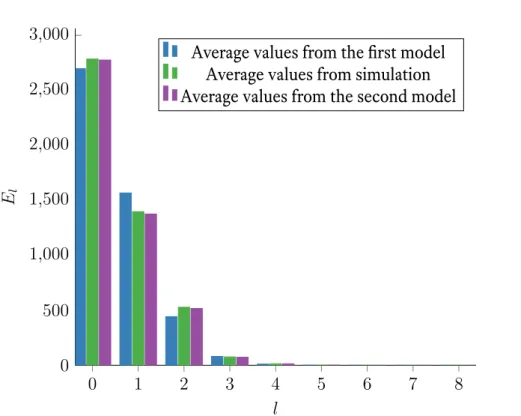
In figure 5.3 we compare the average values of Elat the second iteration with the

val-ues given by the formula in proposition 4.8 and the ones using the transition probabilities we just determined. The probabilities πij for i, j ∈ {0, 1} were determined by running

many simulations. Since we generated the error patterns in the simulations, we know the positions in e∩ f and ¯e∩ f, the counters for those positions, and the values of Elfor all

l.

The formula of proposition 4.8 is a little bit off since it does not take into account that the algorithm tends to decrease the syndrome weight and the error pattern is not random anymore. The bitflipping algorithm tends to decrease the Elvalues for l odd and increase

the Elvalues for l even.

With the newly determined model, we can see that compared to the average values, we tend to slightly underestimate the distributions.

5.2.2 Evolution of the counters

The counters can be studied in a similar way to the syndrome bits.

We use the same notation, we denote by f the set of positions which were flipped and thus, on the second iteration, we will have to decode

s′ = He′⊤ = He⊤⊕ Hf⊤ = s⊕ ∆ with e′ = e⊕ f and ∆ =⊕_j∈fh⊤_j .

Recall that for a position j, the value of its counter is:

CHAPTER 5. DECODING QC-MDPC CODES 28 0 1 2 3 4 5 6 7 8 0 500 1,000 1,500 2,000 2,500 3,000 l El

Average values from the first model Average values from simulation Average values from the second model

Figure 5.3 – Distribution of Elon the second iteration (π00 = 0.00054, π01= 0.31088,

π10= 0.00152, π11 = 0.42507)

So, for the second iteration, it will be

σ_j′ =|h⊤_j ∩ s′| =|h⊤_j ∩ (s ⊕ ∆)

=|(h⊤_j ∩ s) ⊕ (h⊤_j ∩ ∆)|

=|(h⊤_j ∩ s) ⊕ (h⊤_j ∩ ∆ ∩ s) ⊕ (h⊤_j ∩ ∆ ∩ ¯s)| =|h⊤_j ∩ s| − |h⊤_j ∩ ∆ ∩ s| + |h⊤_j ∩ ∆ ∩ ¯s| .

We now define ∆+ _{≜ ∆∩ ¯sand ∆}− _{≜ ∆∩s since they are the part of ∆ responsible}

respectively for an increase and a decrease in the counter values. We also write

σ_j+ ≜ |h⊤_j ∩ ∆+| and σ−_j ≜ |h⊤_j ∩ ∆−| .

We now have σj′ = σj − σ−j + σ

+

j .

In the previous section, we reordered the columns of the matrix H to get a better understanding of the effect of the algorithm on the error pattern after the flips. We do the same thing with the rows.

We suppose that a position j has a counter value σj. We suppose that among the

value. We also suppose that among the syndrome bits which were previously zero but are then flipped, l + k− σjare intersecting with h⊤j and thus increasing the counter value.

In the end the counter value for position j will be σj− k + l + k − σj = l.

s 1 1 |s| 0 0 n− |s| ∆+ 0 0 0 0 1 1 0 0 1 1 ∆− 0 0 1 1 0 0 1 1 h⊤_j ∩ s′ 0 0 0 0 d− l − k 1 1 l + k− σj 0 0 1 1 σj− k 0 0 k h⊤_j ∩ s 0 0 1 1 h⊤_j 0 0 1 1 d− σj 0 0 1 1 σj

Four things can happen between two iterations: — an erroneous position has been flipped; — a good position has been flipped;

— an erroneous position has not been flipped; — a good position has not been flipped.

We therefore choose to condition all the probabilities according to these four situ-ations i.e. for a position j whether j ∈ e or j ̸∈ e and j ∈ f or j ̸∈ f.

Proposition 5.2. We make the hypothesis for all the σj nonzero bits in h⊤j ∩ s the fact that

they will be flipped or not are independent identically distributed Bernoulli trials. Therefore

         σ_j−∼ B(σj, p−11) when j ∈ e ∩ f; σ_j−∼ B(σj, p−10) when j ∈ e ∩ ¯f ; σ_j−∼ B(σj, p−01) when j ∈ ¯e ∩ f; σ_j−∼ B(σj, p−00) when j ∈ ¯e ∩ ¯f .

CHAPTER 5. DECODING QC-MDPC CODES 30

With the following probabilities.

                               p+₁₁≜ P (j ∈ ∆|j ∈ h⊤_j ∩ ¯s, j ∈ e ∩ f) = ∑ j∈e∩fσ + j ∑ j∈e∩fd− σj p+₁₀≜ P (j ∈ ∆|j ∈ h⊤_j ∩ ¯s, j ∈ e ∩ ¯f ) = ∑ j∈e∩ ¯fσ + j ∑ j∈e∩ ¯f d− σj p+₀₁≜ P (j ∈ ∆|j ∈ h⊤_j ∩ ¯s, j ∈ ¯e ∩ f) = ∑ j∈¯e∩fσ + j ∑ j∈¯e∩fd− σj p+₀₀≜ P (j ∈ ∆|j ∈ h⊤_j ∩ ¯s, j ∈ ¯e ∩ ¯f ) = ∑ j∈¯e∩ ¯fσ + j ∑ j∈¯e∩ ¯f d− σj

The same hypothesis can be made for the d− σjother bits in h⊤j ∩ ¯s:

         σ_j+ ∼ B(d − σj, p+11) when j ∈ e ∩ f; σ_j+ ∼ B(d − σj, p+10) when j ∈ e ∩ ¯f ; σ_j+ ∼ B(d − σj, p+01) when j ∈ ¯e ∩ f; σ_j+ ∼ B(d − σj, p+00) when j ∈ ¯e ∩ ¯f .

With the following probabilities.

                               p−₁₁ ≜ P (j ∈ ∆|j ∈ h⊤_j ∩ s, j ∈ e ∩ f) = ∑ j∈e∩fσ−j ∑ j∈e∩fσj p−₁₀ ≜ P (j ∈ ∆|j ∈ h⊤_j ∩ s, j ∈ e ∩ ¯f ) = ∑ j∈e∩ ¯fσ−j ∑ j∈e∩ ¯fσj p−₀₁ ≜ P (j ∈ ∆|j ∈ h⊤_j ∩ s, j ∈ ¯e ∩ f) = ∑ j∈¯e∩fσ−j ∑ j∈¯e∩fσj p−₀₀ ≜ P (j ∈ ∆|j ∈ h⊤_j ∩ s, j ∈ ¯e ∩ ¯f ) = ∑ j∈¯e∩ ¯fσ−j ∑ j∈¯e∩ ¯fσj

Proof. As in the previous section, the assumption that we sum independent identically

distributed Bernoulli trials gives binomial distributions.

Then the probabilities are determined by using the expected values.

We can now determine the transition probabilities between σjand σj′ for any j.

P (σ_j′ = l|σj, j ∈ ¯e ∩ ¯f ) = σj ∑ k=0 ( σj k ) (p−₀₀)k(1− p−₀₀)σj−k ( d− σj l + k− σj ) (p+₀₀)l+k−σj (1− p+₀₀)d−l−k

P (σ_j′ = l|σj, j ∈ ¯e ∩ f) = σj ∑ k=0 ( σj k ) (p−₀₁)k(1− p−₀₁)σj−k ( d− σj l + k− σj ) (p+₀₁)l+k−σj (1− p+₀₁)d−l−k P (σ_j′ = l|σj, j ∈ e ∩ ¯f ) = σj ∑ k=0 ( σj k ) (p−₁₀)k(1− p−₁₀)σj−k ( d− σj l + k− σj ) (p+₁₀)l+k−σj (1− p+₁₀)d−l−k P (σ_j′ = l|σj, j ∈ e ∩ f) = σj ∑ k=0 ( σj k ) (p−₁₁)k(1− p−₁₁)σj−k ( d− σj l + k− σj ) (p+₁₁)l+k−σj (1− p+₁₁)d−l−k When decoding, we are interested in the posterior probabilities. Those can be de-termined using Bayes’theorem.

P (j∈ e|σj, σj′, j ∈ f) = P (σj′|σj, j ∈ e ∩ f) P (j∈ e|σj, j ∈ f) P (σ_j′|σj, j ∈ f) = P (σ_j′|σj, j ∈ e ∩ f) P (j ∈ e|σj) P (σ_j′|σj, j ∈ f)

The same formulas are still true if we change e for ¯eor f for ¯f.

Note that in the bitflipping algorithm, we are interested in knowing when the prob-ability of having an error is greater than the probprob-ability of not having an error. We can therefore take a look at the values taken by

P (j ∈ e|σj, σ′j, j ∈ f) P (j ̸∈ e|σj, σ′j, j ∈ f) and P (j ∈ e|σj, σ ′ j, j ̸∈ f) P (j ̸∈ e|σj, σ′j, j ̸∈ f) .

Using the previous equations, these become:

P (σ′_j|σj, j ∈ e ∩ f)P (j ∈ e|σj) P (σ′_j|σj, j ∈ ¯e ∩ f)P (j ̸∈ e|σj) and P (σ ′ j|σj, j ∈ e ∩ ¯f )P (j ∈ e|σj) P (σ_j′|σj, j ∈ ¯e ∩ ¯f )P (j ̸∈ e|σj) .

In figures 5.5 and 5.4 we compare those theoretical values (in logarithm) for the second iteration with the average values found by simulation. Note that because of the way the counters are distributed, we do not have empirical values for every couple (σj, σj′).

In the bitflipping algorithm, we flip a position when it is more likely to be an error. Here this happens when the ratio is greater than one or when the logarithm of the ratio is positive.

CHAPTER 5. DECODING QC-MDPC CODES 32

0 10 20 30 40

0 20 40

Counter value at the first iteration

Coun ter value at the second it er ation −10 −5 0 5 10

(a) Average values from the model (p+₀₀= 0.14084, p−₀₀= 0.44592, p+₁₀= 0.34323, p−₁₀= 0.20684) 0 10 20 30 40 0 20 40

Counter value at the first iteration

Coun ter value at the second it er ation −10 −5 0 5 10

(b) Average values from simulations

Figure 5.4 – Evolution of the counters between the first two iterations (on average) when the position was not flipped: log

(_{P (j∈e|σ} j,σj′,j̸∈f) P (j̸∈e|σj,σj′,j̸∈f) ) 0 10 20 30 40 0 20 40

Counter value at the first iteration

Coun ter value at the second it er ation −10 −5 0 5 10

(a) Average values from the model (p+₀₁= 0.86216, p−₀₁= 0.55589, p+₁₁= 0.66590, p−₁₁= 0.79448) 0 10 20 30 40 0 20 40

Counter value at the first iteration

Coun ter value at the second it er ation −10 −5 0 5 10

(b) Average values from simulations

Figure 5.5 – Evolution of the counters between the first two iterations (on average) when the position was flipped: log(P (j∈e|σj,σ′j,j∈f)

P (j̸∈e|σj,σ′j,j∈f)

0 10 20 30 40 0

20 40

Counter value at the first iteration

Coun ter value at the second it er ation −10 −5 0 5 10

Figure 5.6 – Threshold curve in function of the previous counter value

5.2.3 Improving proposed variants

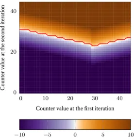
Grey zone In the proposed algorithm for the grey zone bitflipping, the same thresholds as the ones used in [Cha17] are used. But in this algorithm, only a small portion of the positions are selected, and because they are selected on their counter value at the first it-eration, their counters at the second iteration will be distributed differently. For example in the figure 5.6 we can see the values of log

(_{P (j∈e|σ}

j,σ′j,f )

P (j̸∈e|σj,σ′j,f )

)

after the first iteration. It ap-pears that, rather than choosing the same threshold for all the positions, the curve in red is a better choice for the second iteration. This curve delimits the smallest counter values at the second iteration for which the logarithm is greater than zero i.e. such that

P (j ∈ e|σj, σj′, f ) > P (j ̸∈ e|σj, σj′, f ).

We can see that for the second iteration, if we kept track of the previous counters, we can use the best threshold which can range from 23 to 31 with the chosen parameters. Keeping track of the previous counters might be expensive if we do it for all the positions. But in the grey bitflipping algorithm we already restrict ourselves to a few positions, so it might be better to use different thresholds for the grey iterations.

A smaller threshold for the previously flipped position could help detecting early the bad flips (the good positions that were flipped). This could accelerate the algorithm by reducing the number of grey iterations needed and potentially increase the efficiency of the grey zone algorithm.

Multi-bitflipping In the multi-bitflipping algorithm, we estimate the probability of a

position to be an error knowing all its past counter values. The model we now have for the transition probabilities of the counters can be used to replace the empirical choice made for the function f .

CHAPTER 5. DECODING QC-MDPC CODES 34

In a way, the multi-bitflipping is a discretisation of this algorithm 5 which computes the values of:

log ( P (j ∈ e|yj, σj(0), . . . , σ (I) j ) P (j ̸∈ e|yj, σ (0) j , . . . , σ (I) j ) )

where σ(I)_j is the value of the counter at the position j for the I-th iteration. In this algorithm we keep track of the values of the counters at the previous iteration σ′j.

Algorithm 5 The multi-bitflipping algorithm

procedure Multi-bitflipping(y, H) ▷ y = (y1, . . . , yn)∈ {0, 2b− 1}n z ← ( log ( P (e1=1|y1) P (e1=0|y1) ) , . . . , log ( P (en=1|yn) P (en=0|yn) )) ∈ Rn σ← (0, . . . , 0) ▷ H = (h1, . . . , hn)∈ {0, 1}k×n σ′ ← (0, . . . , 0) while Hy⊺ ̸= 0 do s← Hy⊺ for j = 1, . . . , n do σ′_j =⟨s, h⊤_j ⟩_Z (yj, zj)← f(yj, zj, σj, σj′) σj = σ′j return y

The transition probabilities we determined can be used to determine those values. We can suppose that

P (σ(I+1)_j |j ∈ e, f, yj, σ (0) j , . . . , σ (I) j ) = P (σ (I+1) j |j ∈ e, f, σ (I) j ) and P (σ(I+1)_j |j ̸∈ e, f, yj, σj(0), . . . , σ (I) j ) = P (σ (I+1) j |j ̸∈ e, f, σ (I) j ) .

Therefore, the ratio we are looking for can be determined with the following formula using Bayes’ theorem.

P (j ∈ e|yj, σ(0)j , . . . , σ (I+1) j ) P (j ̸∈ e|yj, σ (0) j , . . . , σ (I+1) j ) = P (σ (I+1) j |j ∈ e, f, σ (I) j ) P (σ_j(I+1)|j ̸∈ e, f, σ(I)_j ) P (j ∈ e|yj, σ(0)j , . . . , σ (I) j ) P (j ̸∈ e|yj, σ (0) j , . . . , σ (I) j )

The ratio will be inverted if we flip the position j.

Hence we can therefore choose the function f as follows.

f (y, z, σ, σ′) =    (1− y, −(z + log ( P (σ|j∈e,f,σ′) P (σ|j̸∈e,f,σ′) ) ) if z + log ( P (σ|j∈e,f,σ′) P (σ|j̸∈e,f,σ′) ) > 0 (y, z + log ( P (σ|j∈e,f,σ′) P (σ|j̸∈e,f,σ′) ) ) otherwise .

Rather than relying on empirical values to determine the function f in the multi-bitflipping algorithm, this algorithm may be used to systematically find a multi-multi-bitflipping for a given precision by approximating it.

To get an idea of the limit in terms of decoding failure rate that we can expect with that kind of algorithm, I implemented it in heavily idealised conditions. When we generate an instance we know the error pattern and thus we can keep track of which position is an error and whether it was flipped or not. Therefore we can compute all the probabilities

p+_ij and p−_ij for i, j = 0, 1 specifically for a given iteration of a given decoding instance. This can be used to compute the probabilities needed to define the function f .