HAL Id: hal-02350429
https://hal.archives-ouvertes.fr/hal-02350429
Submitted on 6 Nov 2019
HAL is a multi-disciplinary open access archive for the deposit and dissemination of sci-entific research documents, whether they are pub-lished or not. The documents may come from teaching and research institutions in France or abroad, or from public or private research centers.
L’archive ouverte pluridisciplinaire HAL, est destinée au dépôt et à la diffusion de documents scientifiques de niveau recherche, publiés ou non, émanant des établissements d’enseignement et de recherche français ou étrangers, des laboratoires publics ou privés.
Alexander Hartmann, Gregory Nuel
To cite this version:
Alexander Hartmann, Gregory Nuel. Estimating causal effects using triplet orderings: scale free graphs and dependence on the node order. Journal of Physics: Conference Series, IOP Publishing, 2018, 1036, pp.012002. �10.1088/1742-6596/1036/1/012002�. �hal-02350429�
Content from this work may be used under the terms of theCreative Commons Attribution 3.0 licence. Any further distribution of this work must maintain attribution to the author(s) and the title of the work, journal citation and DOI.
Estimating causal effects using triplet orderings:
scale free graphs and dependence on the node order
Alexander K. Hartmann
Institut of Physics, University of Oldenburg, 26111 Oldenburg, Germany E-mail: [email protected]
Gregory Nuel
LPMA, CNRS 7599, Universit´e Pierre et Marie Curie, Paris, France
Abstract. For many data analysis tasks, obtaining the causal relationships between interacting objects is of crucial interest. Here, the case of modelling causal relationships via causal orderings is considered. Triplet ordering preferences are used to perform Monte Carlo sampling of the posterior causal orderings originating from the analysis of experiments involving observation as well as, usually few, interventions, like knockouts in case of gene expression. The performance of this sampling approach is compared to a previously used sampling via pairwise ordering preference as well as to the sampling of the full posterior distribution. This is performed for artificially generated causal, i.e. directed acyclic graphs (DAGs) with a scale-free structure, i.e. a power-law distribution for the out-degree. The sampling using the triplets ordering turns out to be superior to both other approaches, similar to our previous work, where the less-realistic case of Erd˝os-R é nyi random graphs was considered.
1. Introduction
When analysing large sets of data, on important task is to identify causal relationships [1] between the objects described by the data. One example is the analysis of gene regulatory networks, which have received a great deal of attention. In this context, Gaussian models like the Graphical Lasso [2] or approaches based on mutual information [3] are very popular for inferring gene regulation networks.
When time series of the data are available, the Granger causality [4] is a common approach in general. If time-resolved gene-expression data is available, methods like dynamic Bayesian networks [5] or ordinary differential equations [6] can be applied. Nevertheless, in many cases the temporal resolution is too coarse or it is not at all possible to measure time series. For this case, another popular approach, following the work of Pearl [1], focuses on causal Gaussian Bayesian networks. One can retrieve bounds on causal effects and thus partially determine causal relationships using only observational data [7]. To go beyond this, one can perform intervention calculus [8]. This means in real or numerical experiments, through suitable manipulations, one assigns to selected variables some fixed values. Therefore, they are not affected by the standard dynamics of the systems, while their state value is still available to their interaction
partners. Examples are gene knockouts or gene knockdowns in gene regulatory networks.
treatments. In this paper we focus on estimating causal Bayesian networks in the presence of arbitrary mixtures of (non-time resolved) observational and interventional data [9, 10], i.e. wild-types and knockout/down experiments with possibly multiple interventions within each experiment.
As explained in Ref. [9] estimating the underlying DAG (Directed Acyclic Graph) structure of a causal Bayesian network is equivalent to finding of the so-called causal ordering between the genes of interest. In general, this causal ordering is unknown and belongs to a very large ordering space (p! possible orderings for p genes) which cannot be explored exhaustively. The solution suggested by Ref. [9] consists in sampling causal orderings in the posterior distribution using Markov chain Monte Carlo (MCMC) simulations.
At each MCMC step, a new causal ordering is sampled according to a proposal distribution (for example the Mallows distribution) and the maximum likelihood of the model must be computed given the new ordering to accept or reject the sampled ordering. Thanks to the closed formulas developed in Ref. [9], this likelihood maximisation can be done exactly and efficiently but requires a computational effort which still grows with the sixth power of the number p of interacting objects (e.g. genes). Thus, each single Monte Carlo step is computationally rather expensive.
Mathematically a proper MCMC is guaranteed to converge to the correct sampling, but only on diverging time scales. Given that for practical applications one only has a finite amount of computational resources available, only small networks can be treated in this way. For this reason, an approximation based solely on pairwise probabilities of ordering preference has recently been introduced [11]. This resulted in a considerable increase of efficiency, but led in many cases to less reliable parameter estimates.
Recently, we have extended [12] this approximation to triplet probabilities. We have shown that this results in a strongly increased accuracy with respect to the pairwise approach. Also we have shown that, when allocating a comparable amount of the numerical resources for the two algorithms, the triplet approach outperforms the sampling approach based on the full maximum likelihoods. Nevertheless, the past study was performed for Erd˝os-R é nyi random graphs [13], which is the most simple graph model, showing no structure at all, resulting, e.g., in a Poisson degree distribution. For real systems the underlying graphs usually have a more complicated structure, [14] often resulting in a scale-free, i.e. power-law, degree distribution. For this reason, we have applied the pair- and triplet-based approaches to scale-free graphs. The most important results are that the approximations still outperform the full MCMC sampling and that the triplet-based approach is again better than the pair-based one. Also, we investigated which influence the out-degree of the manipulated node has on the amount of information about the causal structure obtained for the graph.
2. Model and Algorithms
First, we will present the graphical model which is behind this approach. Next, we show how model parameters are estimated by using likelihood calculation and how interventions are incorporated into the scheme. These two sections summarise the detailed descriptions of Ref. [9]. Next, we explain sampling of causal orderings, which we used to establish the causal structure. This allows us to calculate averages of the estimated quantities. Finally, we show how pair- and triplet-approximations are used to speed up the sampling procedure. For the convenience of the reader, this section contains a sufficient amount of details to allow for an implementation of the method and follows closely the presentation in Ref. [12].
2.1. Model
Here, we study directed graphs G = (V, E) with p nodes i∈ V . Pairs of nodes i, j are connected by directed edges (i, j) ∈ E, with weights wi,j. The matrix W = (wi,j) contains all weights.
A nonzero weight describes a causal relationship. We assume that the graph is acyclic, i.e. a DAG. Without loss of generality, we can assume that the nodes are ordered according the causal relationships, i.e. wi,j > 0⇒ i < j. This means within the following random process only nodes
i can have causal effects on nodes j if i < j:
To each node j = 1, . . . , p a Gaussian random variable Xj is associated given by
Xj = mj+
!
i<j
wi,jXi+ !j with !j ∼ N(0, σ2j) . (1)
Thus, the equations are deterministic except the term !j which generates fluctuations of the
variables, e.g., for fluctuations of gene expression and σ2
j determines the strength of fluctuations.
In particular, the parameters m = (m1, . . . , mp) and σ = (σ1, . . . , σp) represent the mean values
and the standard deviations if all interactions were absent. In the following an experiment corresponds to one realisation of the random process (1).
Furthermore, within the model it is possible to perform interventions on the nodes, which assign the variable of a node a fixed value instead of generating the value according to (1). In the DAG these values are used as inputs to the descendants when generating a realisation of the process, i.e. performing an experiment numerically [15].
2.2. Estimating Model Parameters
Given are N experimental data points xk = (xk
1, . . . , xkp) (1≤ k ≤ N) assumed to be generated
according to (1). The set of nodes subject to interventions on experiment k is denoted by Jk, respectively (Jk = ∅ means no intervention for the k’th experiment). We denote by
Kj ={k | j &∈ Jk} the experiments where there was no intervention on node j and by Nj =|Kj|
the number of times node j was not target of an intervention. The log-likelihood of the joint experimental outcome given the parameters has been derived in detail in Ref. [9]. Here we only state the final result for brevity:
#(m, σ, W) = −log(2π) 2 ! j Nj − ! j Njlog(σi)− 1 2 ! j 1 σ2 j ! k∈Kj (xkj − xkWeTj − mj)2, (2)
where eTj denotes the transpose of the unit vector which has a value 1 in position j and
zero entries everywhere else. Note in order to write this equation in the standard form
of the multinomial distribution, one uses the covariance matrix Σ = LTdiag(σ2)L, where
L = (I− W)−1 and I = diag(1) [9]. The above stated form is more convenient, because it
is already diagonal. We omit the dependence of # on the data here for brevity of notation. For the given N measurements, the parameters ˆm, ˆσ, ˆW leading to the maximum likelihood estimator (MLE)
#max= #( ˆm, ˆσ, ˆW) = max
m,σ,W#(m, σ, W) (3)
can be obtained [9] in a straightforward way by the following procedure: First one obtains for each experiment k = 1, . . . , N the measurements normalised with respect to the experiments where there was no intervention on node j, for each node j:
yk,j = xk− 1 Nj
!
k!∈Kj
xk!. (4)
Next one solves the linear system of size p(p− 1)/2 ! i!|i!<j ˆ wi!,j ! k∈Kj yik,jyk,ji! = ! k∈Kj yik,jyjk,j for i < j, 1≤ i, j, ≤ N (5)
to obtain estimates ˆwi,j of the weights for the MLE. Solving a linear system with O(p2) variables
takes O(p6) steps. From this solution one obtains, still just following [9], estimates of the mean
values ˆ mj = 1 Nj ! k∈Kj (xkj − xkWeˆ Tj) (6)
and of the variances
ˆ σj = 1 Nj ! k∈Kj (yk,jj − yk,jWeˆ Tj)2. (7)
2.3. Estimating the Posterior Distribution
So far, we have assumed that the causal ordering of the model is given by o0 = (1, 2, . . . , p).
In experimental situations, if the data was actually generated according the DAG model, the ordering is most of the time unknown, i.e. all estimates will depend on the ordering: #max = #max(o). For the general case, if the data was not generated according to a DAG
model, the modelling must involve many orderings. Thus, in experiments and subsequent model estimation, one is actually interested in either the ordering which maximises the MLE, or, alternatively, in obtaining the posterior distribution involving all (or the dominant) orderings weighted by the corresponding ordering-dependent MLEs.
Both can be obtained in principle by iterating over all p! possible causal orderings o, i.e. permutations of the natural numbers 1, . . . , p. Each time one has to reorder the measurement data according this ordering, and to obtaine the MLE (3) via solving (4), (5), (6) and (7). Clearly, if p is too large, this enumeration is not feasible any more.
One alternative approach is to use a MCMC simulation, where orderings o(t) according the likelihood exp(#max(o)) are sampled, t denotes the number of steps. A convenient approach to
achieve this is the Metropolis algorithm. Here, within each step, a trial order o# is generated. For the present study, we use local changes, i.e. an exchange of the order of two nodes with respect to the current ordering o(t). The trial ordering is accepted, i.e. o(t + 1) = o# with the probability
pacc= min{1, exp[#max(o#)− #max(o(t))]} . (8)
Otherwise, the trial ordering is not accepted and the current ordering kept for the next time step, i.e. o(t + 1) = o(t). Note that for all simulations we performed (see below for details), the empirical acceptance rate of these locally generated trial orderings was below 0.5. The value of 0.5 is considered as a good choice by rule of thumb, balancing a desired high rate of changeing with a desired high acceptance rate. Therefore it would not make sense to consider trial orderings which differ from the current ordering by more than two exchanged positions, since this would increase the fluctuations and therefore decrease the acceptance rate even more. This type of sampling guarantees, in principle, if the Markov chain is long enough, that the orderings are sampled according the desired posterior distribution. Note that for the computation of the change #max(o#)− #max(o(t)) of the log-likelihood one has to recalculate
the log-likelihood for the trial ordering o# from scratch. Thus, each MCMC Metropolis step takes O(p6) running time.
By starting with a random ordering o(0), performing a “long enough” MCMC sampling and by discarding the “initial” part (allowing for equilibration), a sample set S of orderings is obtained, which can be used to calculate averaged estimated parameters, see Section 2.4. 2.4. Calculation of Averaged Estimates
The aim is to study expectation values in ensembles defined by probabilities or likelihoods P (o). Here we are interested in the true likelihoods P (o)∼ e"max(o). Thus, for any measured quantity
A(o), where the estimate depends on the assumed ordering o, the expectation value is given by
(A) ≡!
o
A(o)P (o). (9)
Note that the measured quantities of interest are usually estimates which are obtained from the maximum-likelihood calculation, e.g. the estimates of the weights obtained from (5) or estimates of the variances (7), or any other derived value.
If only a finite set S of samples is given, averages can be obtained, approximating the expectation values: ˆ A≡ " o∈SA(o)P (o) " o∈SP (o) (10) These estimates are most accurate if the process used to generate the sample set follows the desired sampling P (o)∼ e"max(o)as close as possible. Thus, the sample set S could be generated
by a MCMC sampling according to the true probabilities e"max, as outlined in the previous
section. In this way automatically orderings with high contributions to (10) are preferentially generated. Note that since S is actually a mathematical set, there will be no multiple occurrences of orderings in S. If one allowed for multiple occurrence, then one would have to take simple arithmetic averages instead of weighted ones as in (10).
Anyway, here we work with sampling sets. The reason is that, alternatively, these sets can be obtained by sampling according to different probabilities, which only aim at approximating the true probabilities but which are computationally much cheaper to calculate. (This also means, we accept a sampling error, which would only disappear if the sampling set approaches the set of all possible configurations). One the other hand, if the size of the set is suitably restricted, we used always|S| = 100, the computationally expensive O(p6) full likelihood calculations have
to be performed only for a small number of (here) 100 samples.
The approximate probabilities we have used are introduced in the following section. 2.5. Pair and Triplet Probabilities
Instead of sampling the full posterior distribution, in Ref. [11] it was proposed to perform an MCMC sampling from a different distribution, the Babington-Smith (BS) ordering distribution [16, 17]. It is based on pair preferences πi,j (1 ≤ i &= j ≤ p) with πi,j ∈ [0, 1] and
πi,j + πj,i = 1. The meaning is that within the desired ordering distribution in any random
ordering element i appears before j with this probability πi,j. The pair preferences can be
estimated from the experimental data with interventions by considering all possible two-node graphs Gi,j ≡ ({i, j}, {(i, j)}) with the nodes i and j and with exactly one directed edge (i, j).
As above, for brevity of notation, we omit the dependence of the pair preferences and any derived quantities on the data here. Only the data values for the two nodes are considered. Note that in case of multiple interventions, we observed in tests, which are not contributing to the results shown here, that the overall performance of the sampling according pair preferences is somehow better if data points with interventions on other nodes than i, j are not included in the data set for the pair i, j, respectively. For each of the p(p−1) directed two-node graphs the log-likelihood #(2)max(i, j) is obtained. The pair preferences are then given by
πi,j = exp(#
(2) max(i, j))
exp(#(2)max(i, j)) + exp(#(2)max(j, i))
. (11)
From the pair preferences, the BS probability of a full ordering o is obtained by
P (o|π) ∼#
i<j
with a suitable normalisation. The normalisation is not needed here, since, first, we only compare the (relative) values of (12) for different orderings. The corresponding log-likelihoods are denoted as
#pair≡ #pair(o) = log#
i<j
πoi,oj. (13)
Second, we performed MCMC sampling of orderings using the Metropolis algorithm according to (12) where also only relative likelihoods are needed. This was done in an equivalent way as above, only the true MLE is replaced by (13). Thus, starting again from a random ordering o(0), we generated trial orderings o#by exchanging the i-th and the j-th entry in the current ordering. The new orderings are accepted with the corresponding Metropolis probability. Note that one does not have to recalculate the BS probability from scratch, since the change in probability is easier to obtain. The Metropolis acceptance probability is given by
ppairacc = min
1, πoj,oi πoi,oj # k|i<k<j πoj,okπok,oi πoi,okπok,oj . (14)
This takes only O(p) steps compared to the O(p2) steps which are needed for the calculation of the full probability. In particular it is much faster than computing the full likelihood which takes O(p6) steps.
Naturally, when sampling according to (12) the observed set of orderings will be different but somehow similar to when sampling according the true likelihood. The reason is that orderings with a high full likelihood induces in principle large pairwise probabilities for those pairs which are compatible with such an order. Nevertheless, the pairwise approximation cannot completely cover collective effects which involve the ordering of more than two nodes. Thus, the final estimates, like the weights, for the posterior distribution are obtained by keeping the nincl
samples with the highest probabilities (12) in the sample set S. For these orderings now the true MLE (3) is evaluated and used. This means, (10) is applied for any kind of estimation or averaging, i.e. these weights are now used in this final averaging step.
In [11] it was found that this sampling approach is in some case similar accurate as a full MCMC sampling as described in Sec. 2.3, but there were notable differences. In particular when the number p of nodes is growing, the orderings exhibiting the largest pair-based probabilities turned out to be more and more different from the orderings exhibiting large full likelihoods. This showed up in particular when calculating estimates of network parameters. Therefore it was proposed to maybe consider triplets instead of pairs.
Thus, it is the purpose of the present work to study this higher level approximation of the true posterior distribution. Similar to the above defined pair probabilities, we introduce triplet probabilities ρi,j,k ∈ [0, 1] such that ρi,j,k + ρi,k,j + ρj,i,k + ρj,k,i + ρk,i,j + ρk,j,i = 1
(i < j < k). These probabilities can be estimated from the experimental data in a similar way as above, by considering all possible sub graphs ({i, j, k}, {(i, j), (i, k), (j, k)}) with three nodes and corresponding edges. For these sub graphs the corresponding MLE are obtained and suitably normalised, equivalent to (11) to yield the triplet probabilities ρi,j,k. They can be used
to generalise the Babington-Smith probabilities of orderings to
P (o|ρ) ∼ #
i<j<k
ρoi,oj,ok. (15)
Again, the normalisation is not needed here. The corresponding log-likelihood is denoted as #tripl= log #
i<j<k
We perform an MCMC sampling of orderings according to these probabilities using the Metropolis algorithm and trial ordering generated via swapping of pairs of elements. Like for the case of sampling according the pair-based probabilities, these swapping pairs are chosen unbiased, i.e. each pair is chosen with the same probability. To guarantee a sampling according to (15), for the calculation of the acceptance probabilities only the change in probability of (15) has to be considered, which now takes O(p2) steps for such a swap.
Again, for all evaluations and estimates, the nincl = 100 highest-probability samples with
respect to the triplet probability are kept. For these samples the true likelihood is obtained and used for all averaging processes according to (10).
3. Results
We have performed simulations for scale-free random DAGs with p nodes. The graphs are generated similarly to the Barab á si-Albert model [14] with iterated preferential attachment of each node to m (m = 3 or m = 4 here) already existing nodes. Note that for the original undirected model, the graph generation starts with a complete graph with m + 1 nodes. Here, to obtain a DAG, the initial graph consists of m+1 nodes such that node 1 is connected by directed edges (1, j) to the other nodes j = 2, . . . , m + 1. Then, iteratively the nodes j = m + 2, . . . , p are added to the graph. Each new node j is connected to m randomly chosen nodes among the already existing nodes k = 1, . . . , j− 1 by directed edges (k, j). The probability that the new node is connected to an existing node by an edge is proportional to the degree (sum of in-degree and out-degree) of the already existing node.
Each edge receives a weight which is drawn uniformly from the range [−1, −0.4] ∪ [0.4, 1]. Thus, these edges should be distinguishable very well from the absent edges which correspond to weight 0. Finally, for each DAG instance, for each node j, mean values mj = 1/2 are used
and the variance values σj are drawn randomly uniformly in the interval [0.01, 0.1]. In Ref. [12]
we have shown that the choice of mj and σj does not play a crucial role. All simulations are
performed for 1000 (p = 20) and 300 (p = 50) DAG instances generated independently in this way.
Next, for each DAG instance, a certain number of N measurements are performed, where the measurement vectors xk (k = 1, . . . , N ) are generated according to (1). Typically, for a DAG
of p nodes, we generated N = 10p measurement vectors. Note that the scheme exhibited in Section 2.2 allows for multiple interventions. Nevertheless, since we are interested in comparing different sampling approaches here, we present for simplicity just single interventions which are systematically done during the first r (r ≤ N) experiments of each set of experiments. We applied a systematic manner, such that for all nodes at least,r/p- interventions are performed while for r− p,r/p- nodes one intervention more, i.e. .r/p/ interventions are performed. This sums up to r interventions. For each intervention on node j, we fix Xi = 0, respectively,
corresponding to a knockout. For the order in which the nodes are taken for interventions (experiment by experiment), we studied three different variants:
• decreasing out-degree • random order
• increasing out-degree
This means for decreasing order, in experiment 1, the node with the highest out-degree will be set to zero, in experiment 2 the node with the second highest out-degree, and so on.
Thus, to measure the efficiency of an approach, we consider all edge weights wi,j, where wi,j
might be zero because it does not match the causal ordering, or because the causal interaction is just absent. This is done in the following way: From each sampling, we obtain averaged estimated
edge weights ˆwi,j (i, j = 1, . . . , p) according to (10). Now, we count the “bad” estimates of the
edge weights by comparing with the true edge weight as follows: δbad(i, j) = * Θ(| ˆwi,j| − w0) if wi,j = 0 Θ+,,,wi,j− ˆwi,j ˆ wi,j , , , − w1 -if wi,j &= 0 . (17)
Θ(x) denotes the threshold function which is Θ(x) = 0 for x ≤ 0 and Θ(x) = 1 for x > 0. Thus, for a weight which is zero in the original DAG used to generate the data, the averaged estimate is counted as bad if its absolute value exceeds a threshold value w0. For an edge
with nonzero weight of the original DAG the average estimate is counted as bad, if the relative deviation of the average estimated weight and the original weight exceeds threshold value w1.
We used w0 = 0.1 and w1 = 0.5. In general, details of the results might depend on the actual
values of w0 and w1, but we verified that the principal trends, with respect to which sampling
approach performs better, remain the same [12]. Also when using the threshold-independent area under the Receiver-Operator Characteristics (ROC), the principal nature of the results does not change [12]. Thus, we concentrate here on estimating the “bad” edges by iterating over all edges, i.e. we measured
nbad= 1 p(p− 1) ! i$=j δbad(i, j) . (18)
3.1. Comparing Different approaches
First, we compare the performance of the four different approaches, i.e. when using the original ordering, sampling orderings with MCMC based on the full likelihood, sampling with pair probabilities and sampling with triplet probabilities.
0 0.1 0.2 0.3 0 1 2 3 4 5 6 7 8 9 nbad r/p p=20 nodes scale free graphs N=200 experiments full (2ttripl) pairs triplets exact 0 0.05 0.1 0.15 0.2 0 1 2 3 4 nbad r/p p=50 nodes scale free N=500 exper. full (2ttripl) pairs triplets exact
Figure 1. Average fraction nbad of incorrectly estimated edge weights as a function of the number of
interventions r per node. The results are obtained using four different sampling approaches using the true maximum likelihoods (full), the pair BS probabilities (pair), the triplet BS probabilities (triplet) and using just the exact ordering of nodes of the DAGs. The running time for the sampling using the true maximum likelihoods was restricted to two times the CPU time of the triplet sampling. (left) The data was generated for 1000 randomly generated scale free DAGs (m = 3) of size p = 20 nodes. (right) Results for 200 scale free DAGs (m = 4) of size p = 50.
In Fig 1 (left) the resulting average values for the fraction nbadof incorrectly estimated edge
r/p of single-node interventions. The order in which the nodes are fixed was random. One can observe that with increasing number of interventions, the quality of the averaged weight estimate increases. Similar to the case of complete graphs [12], due to the limited number of MCMC steps performed, sampling using the true likelihoods is the worst approach, except for a very small number of interventions, where the estimates are bad anyway. For scale-free graphs the quality of the estimates is much better when using the triplet probabilities as compared to the pair probabilities. Still, one cannot reach the quality of the estimate which we obtained when using the single true ordering, which constitutes the lower limit of what is achievable using any algorithm.
We have repeated the same study for larger graphs of p = 50 nodes, here for m = 4. Again we have measured the fraction nbad of incorrectly estimated edge weights. In Fig. 1 (right) the
corresponding results are shown. The results for the triplet-based approach are better than for the pair-based method, and much better than the full MCMC sampling restricted to at most twice the numerical resources of the triplet-based simulation. Note that the difference between pair-based approach and triple-based approach is now larger than for the p = 20, m = 3 case. For p = 50, m = 3 (not shown) the differences are smaller than for p = 50, m = 4. This goes along with the previous results [12] that the difference between pair-based and triplet-based approaches grows with the edge-density of the graphs.
3.2. Influence of node degree
It is a natural assumption that the effect of an intervention on a node is larger for higher number of outgoing edges. For this reason, we have performed simulations for varying order (increasing/random/decreasing degree) of the nodes. Still, for each experiment exactly (at most) one node is fixed to zero. This means in particular that after p experiments, each node has been fixed for exactly one experiment, here the order should have no large influence.
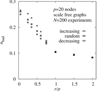
0 0.1 0.2 0.3 0 0.5 1 1.5 2 nbad r/p p=20 nodes scale free graphs N=200 experiments
increasing random decreasing
Figure 2. Average fraction nbad of incorrectly estimated edge weights as a function of the number of
interventions r per node. The data was generated for 1000 randomly generated scale free DAGs of size p = 20 nodes. The results are obtained using the triplet BS probabilities for different orderings of nodes: with increasing out-degree, random, and decreasing out-degree.
The results are shown in Fig. 2. For fixing the nodes with decreasing out-degree, the results for the number nbad of incorrectly estimated edges are best, they are below the results for the
two other approaches. When using the increasing out-degree order, the results are worst. This appears natural, because when fixing nodes with higher degree earlier, one learns the causal structure of a network quicker. Nevertheless for r/p = 1 the results agree within error bars for the three different orders. Also, for r/p > 1 the results are basically indistinguishable. The reason is that each node has been fixed already exactly or at least once. Therefore, the additional information one obtains from fixing a node again is small anyway. This means, the order does not play so much of a role. Note that for r/p = 1 the results should be statistically indistinguishable anyway, because here each node has been fixed exactly for one experiment. Furthermore, the differences between the three approaches are also not very big for r/p < 1. In particular the regime where nbad decreases strongly seems to extend for all three cases up to
r/p = 1. This means in particular, that fixing the nodes in a random order, which corresponds to real situations where the node degrees are not known beforehand, is no real drawback when determining causal structures.
4. Summary and Discussion
To summarise, we studied the estimation of causal orderings and corresponding parameters in sampled data using interventions. In particular, we compared pairwise Babington-Smith sampling, which was discussed before [11] with triplet-based sampling for scale-free graphs. This ensemble is more realistic for real data applications in comparison to Erd˝os-R é nyi random graphs for which these approaches have been compared in a previously published work [12]. All results show a better performance for the triplet sampling approach. When limiting the numerical effort to about two times the running time of the triplet sampling, a sampling using the full maximum likelihood turned out to be much worse than both pair- and triplet-based sampling. Nevertheless, for very sparse graphs, the performance of pair- and triplet-based sampling is more similar.
Therefore, the triplet-based approach and, to some extent, the pair-based approach appear to be well-balanced: They are computationally efficient enough such that long MCMC chains can be generated easily for systems large enough for practical applications. This would be impossible when using a sampling based on the full likelihood, except for very small systems. On the other hand, in combination with the final computation of the true maximum-likelihood estimators for a comparable small subset of “best” configurations, the triplet approach allows for accurate results, in some cases much — in other cases slightly — better than the pair-based approach.
For future work it will be interesting to extend the approaches to very large networks. There exist other approaches for the estimation of the causal structure of actually very large networks of thousands of nodes using ad hoc heuristic algorithms [18, 19] which are based, among others, on clustering approaches and work often on a coarse-grained level. Although the approaches presented here are based on generative models, allowing for probabilistic interpretations and allowing for detailed reconstruction of the underlying networks, they can be extended to much larger systems as well. This can be achieved for a given large set of nodes by considering many different subsystems (subgraphs) of medium size and treating them with the correct joint likelihoods. The resulting sub networks can be assembled to one large consensus network. Here, e.g. the “Iterative Sub-Network Component Analysis” approach [20] or similar approaches can be applied.
Furthermore, it could be interesting to study more thoroughly the point r = p where most results exhibit a notable change of characteristics: For r < p the progress when adding further interventions is much faster compared to r > p. It could be interesting whether this change corresponds to a kind of information-driven “learning” phase transition, similar to Hopfield neural networks where the memory does not work well beyond a certain number of patterns to be stored.
than one node per experiment. Also adaptive schemes could be useful, where the choice of the next intervention node depends on the outcome of the previous interventions.
Acknowledgments
We thank Hendrik Schawe for critically reading the manuscript. A visit of GN to the University of Oldenburg, during which the project was set up, was supported by the Graduiertenkolleg 1885 “Molecular Basis of Sensory Biology” funded by the Deutsche Forschungsgemeinschaft (DFG). AKH is grateful to the Foundation Sciences Math´ematiques de Paris (FSMP) for providing financial support for a three month (February to April 2016) visit at the LPTMA of the Universit´e Pierre et Marie Curie during which this project was designed and started.
The simulations were performed on the Carl cluster of the University of Oldenburg jointly funded by the DFG (INST 184/157-1 FUGG) and the Ministry of Science and Culture (MWK) of the Lower Saxony State.
[1] Pearl J 2009 Causality (Cambridge: Cambridge University Press) [2] Friedman J, Hastie T and Tibshirani R 2008 Biostatistics 9 432–441
[3] Wang J, Chen B, Wang Y, Wang N, Garbey M, Tran-Son-Tay R and et al 2013 Nuc. ac. res. 41 e97 [4] Granger C W J 1969 Econometrica: J. Econ. Soc. 37(4) 424–438
[5] Zou M and Conzen S D 2005 Bioinf. 21 71–‒ 79
[6] Wu H, Lu T, Xue H and Liang H 2014 J. Amer. Stat. Assoc. 109 700 ‒ –716
[7] Maathuis M H, Colombo D, Kalisch M and B¨uhlmann P 2010 Nature Methods 7 247–248 [8] Maathuis M H, Kalisch M and B¨uhlmann P 2009 Annals Stat. 37 3133–3164
[9] Rau A, Jaffr´ezic F and Nuel G 2013 BMC systems biology 7 1
[10] Hauser A and B¨uhlmann P 2015 J. Royal Stat. Soc.: Series B 77 291–318 [11] Nuel G, A A R and Jaffr´ezic J 2014 Quality. Techn. Quant. Manag. 11 23–37 [12] Hartmann A K and Nuel G 2017 PLOS one 12 e0170514
[13] Erd˝os P and R´enyi A 1960 Publ. Math. Inst. Hungar. Acad. Sci. 5 17–61 [14] Albert R and Barab´asi A L 2002 Rev. Mod. Phys. 74 47
[15] Hartmann A K 2015 Big Practical Guide to Computer Simulations (Singapore: World Scientific) [16] Critchlow D E, Fligner M A and Verducci J S 1991 J. Math. Psych 35 294–318
[17] Joe H and Verducci J S 1993 Cell 102 109–126
[18] Liang T L H and Li H 2011 J. Amer. Stat. Assoc. 106 1242–1258
[19] Wang Y, Xu M, Wang Z, Tao M, Zhu J and et al L W 2011 Brief. Bioinform. 13 162–174 [20] Jayavelu N D, Aasgaard L S and Bar N 2015 BMC Bioinf. 16 366