Bunching at the kink: Implications for spending
responses to health insurance contracts
The MIT Faculty has made this article openly available.
Please share
how this access benefits you. Your story matters.
Citation
Einav, Liran, Amy Finkelstein, and Paul Schrimpf. “Bunching at the
Kink: Implications for Spending Responses to Health Insurance
Contracts.” Journal of Public Economics 146 (February 2017): 27–40.
As Published
http://dx.doi.org/10.1016/J.JPUBECO.2016.11.011
Publisher
Elsevier BV
Version
Author's final manuscript
Citable link
http://hdl.handle.net/1721.1/120358
Terms of Use
Creative Commons Attribution-NonCommercial-NoDerivs License
Bunching at the kink: implications for spending responses to
health insurance contracts
Liran Einav,
Department of Economics, Stanford University, and NBER, [email protected]
Amy Finkelstein, and
Department of Economics, MIT, and NBER, [email protected]
Paul Schrimpf
Vancouver School of Economics, University of British Columbia, [email protected]
Abstract
A large literature in empirical public finance relies on “bunching” to identify a behavioral response to non-linear incentives and to translate this response into an economic object to be used
counterfactually. We conduct this type of analysis in the context of prescription drug insurance for the elderly in Medicare Part D, where a kink in the individual’s budget set generates substantial bunching in annual drug expenditure around the famous “donut hole”. We show that different alternative economic models can match the basic bunching pattern, but have very different quantitative implications for the counterfactual spending response to alternative insurance contracts. These findings illustrate the importance of modeling choices in mapping a compelling reduced form pattern into an economic object of interest.
Keywords
Bunching; Medicare; Health insurance; Health care
1. Introduction
Over the last decade, there has been an increased reliance in public economics on evidence that is based on observed “bunching” around kink points in budget sets; Kleven (2016) provides an overview of this growing literature. The key underlying idea is simple and tractable: if rational individuals face a non-linear budget set with considerable kinks, they should bunch around the kinks, and the extent of bunching should be informative about relevant elasticities (or lack thereof). The existence of bunching or excess mass around kink
Correspondence to: Paul Schrimpf.
Publisher's Disclaimer: This is a PDF file of an unedited manuscript that has been accepted for publication. As a service to our customers we are providing this early version of the manuscript. The manuscript will undergo copyediting, typesetting, and review of the resulting proof before it is published in its final citable form. Please note that during the production process errors may be discovered which could affect the content, and all legal disclaimers that apply to the journal pertain.
4Although, as noted by Manoli and Weber (forthcoming), even in the labor supply context, retirement incentives can create important
HHS Public Access
Author manuscript
J Public Econ
. Author manuscript; available in PMC 2018 February 01. Published in final edited form as:J Public Econ. 2017 February ; 146: 27–40. doi:10.1016/j.jpubeco.2016.11.011.
A
uthor Man
uscr
ipt
A
uthor Man
uscr
ipt
A
uthor Man
uscr
ipt
A
uthor Man
uscr
ipt
points of a budget set can thus provide compelling, visual evidence against the null hypothesis of no behavioral response of individual to the incentives; likewise, the lack of such bunching suggests the opposite.
Many of the applications of this idea have been in the context of the behavioral response to non-linear income tax schedules (Saez, 2010; Chetty et al., 2011; Chetty, Friedman, and Saez, 2013a; Kleven and Waseem, 2013; Bastani and Selin, 2014; Kleven et al., 2014). But similar ideas have been widely applied in other settings that generate non-linear budget sets, including pensions (Manoli and Weber, forthcoming), electricity (Ito, 2014), fuel economy policy (Sallee and Slemrod, 2012), mortgages (Best et al., 2015), cell phones (Grubb, 2015; Grubb and Osborne, 2015), broadband (Nevo, Turner, and Williams, 2016), taxes on home sales (Kopczuk and Monroe, 2015; Best and Kleven, 2016), healthcare procurement (Bajari et al., 2013), and – the subject of this current paper – health insurance contracts (Abaluck, Gruber, and Swanson, 2015; Dalton, Gowrisankaran, and Town, 2015; Einav, Finkelstein, and Schrimpf, 2015).
A likely key factor behind this recent popularity of bunching estimates is the seminal contribution of Saez (2010), which illustrates how one may convert an observed bunching pattern to an economic object of interest: a “structural” behavioral elasticity parameter. Using data on individuals’ annual earning, which bunch around convex kinks in the income tax schedule, Saez used a stylized, static, frictionless model of labor supply to provide a simple, transparent, and easy-to-implement mapping from the observed bunching to an estimate of the elasticity of labor supply (or earning) with respect to the marginal tax rate. This allows one to take the compelling visual evidence of bunching and move beyond merely rejecting the null of non-behavioral response to estimating a quantitative economic object of interest that can be used to predict behavioral responses to counterfactual
scenarios. Not surprisingly, this compelling and tractable idea has been quite influential, and has been frequently used to translate various bunching estimates into “structural” elasticities (Chetty et al., 2011; Kleven et al., 2011; Kleven and Waseem, 2013; Bastani and Selin, 2014).
The Saez (2010) approach is very appealing. It is transparent and easy to implement. Of course, the simplicity comes at the cost of potentially abstracting from a host of real-world features that may be important in a particular context. An alternative to this approach would be to develop a more complete model of a given context, which includes dynamics,
uncertainty, and other relevant frictions. Manoli and Weber (forthcoming) provide such a model in the context of labor supply, and our earlier work (Einav, Finkelstein, and Schrimpf, 2015) provides another example in the context of demand for prescription drugs. As the Saez approach is so much simpler and easier to implement, it seems useful to ask how well of an approximation to the main object of interest, a simpler, Saez-style approach can provide. Naturally, the reasonableness of the approximation will depend on the specific context. This is precisely the goal of the current paper, where we explore this question in the context of demand for prescription drugs under Medicare Part D, the public prescription drug insurance program for elderly and disabled individuals in the United States. Our substantive question concerns the spending (or “moral hazard”) effects of alternative insurance
A
uthor Man
uscr
ipt
A
uthor Man
uscr
ipt
A
uthor Man
uscr
ipt
A
uthor Man
uscr
ipt
contracts. This is a topic that has attracted considerable attention both for health insurance contracts in general, and more recently in our specific Part D context.
We begin in Section 2 by describing the setting and the data. An important feature of Medicare Part D coverage is the donut hole in the basic benefit design, which generates a large, discontinuous increase in the marginal price. Consequently, individuals’ annual drug expenditures bunch around this kink, making it a natural context to explore the implication of different bunching estimates.
In Section 3 we present and estimate two different models of prescription drug purchasing behavior. The first is our adaptation of the static, frictionless Saez (2010) model to the Medicare Part D context; we refer to it hereafter as a Saez-style model and the resultant elasticities as Saez-based elasticities. The second is the dynamic model we developed in our earlier work (Einav, Finkelstein, and Schrimpf, 2015); we refer to it hereafter as the dynamic model and the resultant elasticities as the dynamics-based elasticities. Both models match the basic bunching pattern; however, the implied elasticity from the dynamic model is an order of magnitude greater than the Saez-based elasticity estimate. This is the key result of the paper.
There are multiple differences between the two, non-nested settings. The Saez-style framework assumes continuous spending decisions (i.e. no lumpiness in drug purchases), perfect foresight of future health shocks (i.e. no uncertainty), and no discounting of the future. None of these assumptions are made in the dynamic model. It is interesting to explore which features of the model are most important for the differences in implied elasticities, which is the focus of Section 4. There we develop two modifications of the dynamic model, which bring it closer to the Saez-style framework. We then re-estimate each of these versions of the model using the same data. Our main finding is that a static, perfect foresight version of the full dynamic model – which comes quite close to the Saez-style model except that it allows for lumpiness in spending decisions – results in implied elasticities that are about half way between the Saez-based estimates and the dynamics-based ones. Interestingly, once we allow for lumpiness, allowing for uncertainty essentially allows us to recover the magnitude of the elasticity implied by the full dynamic model; as it turns out, allowing for discounting is not quantitatively important.
We emphasize that the results we present in this paper should be viewed as illustrative. They are specific to our particular (Medicare Part D) context, as well as to the modeling choices we have made. Nonetheless, they highlight what we believe to be an important and broader point: in-sample bunching patterns may be rationalized by a host of modeling assumptions, and these assumptions can, at least in some contexts, have very different quantitative implications for the out-of-sample objects of interest.1 This is a general issue that the “bunching” literature has grappled with: the immense sensitivity of results to the particular modeling assumptions used to translate the observed excess mass at a convex kink into an economic object that can be used in other contexts. Indeed, in an early, working paper
1Kleven (2016) emphasizes a similar point in his review article. In the labor supply context, he describes several empirical papers which show that, with potential optimization frictions, a given excess mass in the earnings distribution can be rationalized with virtually any underlying, “structural” labor supply elasticity.
A
uthor Man
uscr
ipt
A
uthor Man
uscr
ipt
A
uthor Man
uscr
ipt
A
uthor Man
uscr
ipt
version of his original contribution, Saez (1999) shows that the translation of the excess mass at kinks in the US income tax schedule to an underlying labor supply elasticity can be greatly affected by adding to the baseline model either earnings uncertainty or making labor supply choices discrete and lumpy rather than continuous.
This is essentially an under-identification problem, which is more formally characterized by Blomquist et al. (2015), who emphasize the need for additional moments in the data that would allow us to select among models. The subsequent bunching literature has broadly pursued two main strategies for handling this identification issue. One is to use the
frequency of observations in dominated regions of the budget set (“notches”) to identify the extent of frictions; Kleven and Waseem (2013) develop this approach. Another is to parametrize the frictions – or other relevant features of the setting – and use additional moments in the data to identify them. In the working paper version of Chetty et al. (2011), the authors explore such an approach, developing a labor supply model and parametric search costs that have quantitatively important implications for translating observed excess mass into an underlying, “structural” elasticity (Chetty et al., 2009). The exercise in our paper is similar in spirit; our focus is less on “frictions” but more on the dynamic nature of our problem, and we therefore use non-bunching moments, associated with the way spending patterns vary over the calendar year, to identify additional parameters of the dynamic model.
More generally, our paper speaks to the growing interest in our profession in developing approaches to translate compelling, transparent, “reduced form” evidence of a behavioral response into an economic object of interest. The bunching literature following Saez (2010) is one specific application of the influential “sufficient statistics” literature popularized by Chetty (2009) – which attempts to use simple models to directly and transparently map reduced form parameters into welfare analyses. But the phenomenon is more general. For example, randomized controlled trials have the ability to deliver compelling “causal effect” estimates, but translating the experimental treatment effects into economic objects that can be applied out-of-sample to make counterfactual predictions or analyses often requires additional economic modeling assumptions (Aron-Dine, Einav, and Finkelstein, 2013). Our (modest) goal here is to illustrate in a particular context that these modeling assumptions can be quite consequential. As we have demonstrated, two “reasonable” (in our subjective view) alternative models can match the basic reduced form bunching facts, while giving very different out-of-sample predictions. Sufficient statistics, in other words, are sufficient conditional on the model (or a set of models). This is an obvious point, made clearly by Chetty (2009), but it is sometimes forgotten in applications and interpretations.
2. Setting and data
2.1. Setting
The setting for the exercise in this paper is Medicare Part D, the prescription drug coverage component of Medicare that was added in 2006. As of November 2012, 32 million people (about 60% of Medicare beneficiaries) were enrolled in Part D, with expenditures projected to be $60 billion in 2013, or about 11% of total Medicare spending (Kaiser Family
Foundation 2012a, 2012b). Unlike Medicare Parts A and B for hospital and doctor coverage,
A
uthor Man
uscr
ipt
A
uthor Man
uscr
ipt
A
uthor Man
uscr
ipt
A
uthor Man
uscr
ipt
which provide a uniform public insurance package for all enrollees (except those who select into the managed care option, Medicare Advantage), private insurance companies offer various Medicare Part D contracts, and are reimbursed by Medicare as a function of their enrollees’ risk scores.
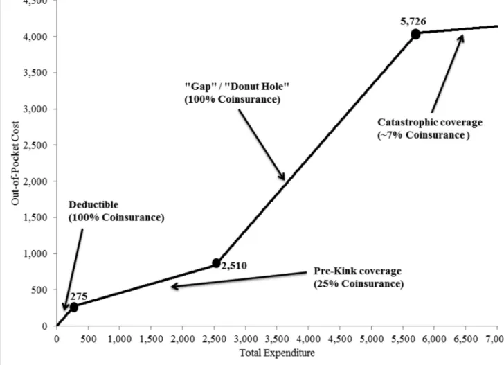
While the exact features of the plans offered vary, they are all based around a government-defined standard benefit design, shown in Figure 1. Our main focus is on the convex kink in the budget set, arising from the discontinuous increase in the out-of-pocket price individuals face when they cross into the “donut hole” (or “gap”; see Figure 1). Standard economic theory suggests that, as long as preferences are convex and smoothly distributed in the population, we should observe individuals bunching at this convex kink point of their budget set. Saez (2010) provides a recent, formal discussion. To see the intuition, consider a counterfactual linear budget set, i.e. the continuation of the co-insurance arm’s cost sharing into the gap. In this case, individual spending would be distributed smoothly through the kink. For example, as illustrated in Figure 2, the solid and dashed indifference curves represent two individuals with different healthcare needs who would have different total drug spending under this linear contract. With the introduction of the kink, however, the spending of the sicker (dashed) individual will decrease and locate at the kink, as would all individuals whose spending under the linear contract was in between the solid and dashed individuals, thus generating “bunching.” In a frictionless world, these individuals would pile up exactly at the kink. In practice, with real-world frictions such as the lumpiness of drug purchases and some uncertainty about future health shocks, individuals are instead expected to cluster in a narrow area around the kink.
2.2. Data
We use data on a 20% random sample of all Medicare part D beneficiaries over the years 2007–2009. The data include basic demographic information (such as age and gender), predicted risk score, and detailed information on the cost-sharing characteristics of each beneficiary’s prescription drug plan. We also observe detailed, claim-level information on our beneficiaries’ Medicare part D utilization during the same years.
We use a sub-sample of the data we used previously in Einav, Finkelstein, and Schrimpf (2015). That data excluded various groups of beneficiaries for whom the empirical strategy is not applicable – such as individuals in Medicare Advantage and certain low income individuals for whom the basic benefit design we study does not apply – and individuals under age 65; see Einav, Finkelstein, and Schrimpf (2015) for a complete discussion and details of the sample. In the current paper, given the more conceptual emphasis and in order to reduce computational burden, we further restrict the sample to a 10 percent random sample of enrollees in the five largest plan-years.
With these restrictions, our final analysis relies on a data set of 27,237 person-years (14,521 unique individuals), which are distributed fairly evenly across the five plans. One plan is in 2007, two in 2008, and two in 2009. One plan is similar to the standard contract described earlier, with approximately 20 percent cost sharing prior to the gap. The four other plans have no deductible, but require enrollees to pay 35–40 percent (depending on the plan) prior to the gap. None of the plans provides coverage in the gap, leading to a sharp kink as
A
uthor Man
uscr
ipt
A
uthor Man
uscr
ipt
A
uthor Man
uscr
ipt
A
uthor Man
uscr
ipt
described earlier. The average age in our sample is 76, and about two thirds of the
individuals are females. Average annual, per-beneficiary drug spending is $1,853 dollars, out of which $834 are paid (on average) out of pocket. Spending is very right skewed: 4.5% of beneficiaries have no annual drug spending, median spending is about $1,391, and the 90th percentile is about $3,689. The exact location of the kink, as a function of total drug spending, also varies across observations in our sample depending on the year, but on average it hits at roughly the 75th percentile of the drug spending distribution. On average, in our sample, the out of pocket price increases from 0.35 to 0.99 at the kink.
2.3. Bunching
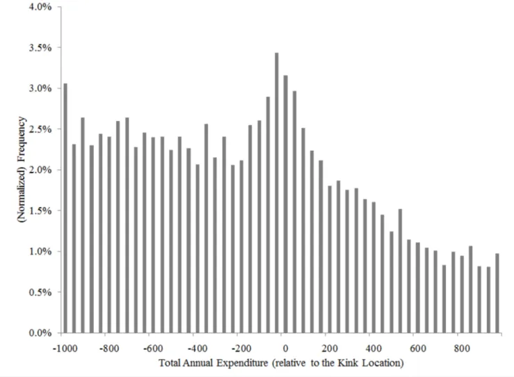
Bunching at the kink is clearly evident in the raw data. Figure 3 provides the motivation and starting point for the analysis in the rest of the paper. Because the kink location has changed from year to year (from $2,400 in 2007, to $2,510 in 2008, and $2,700 in 2009), in all our analysis we normalize annual spending by the kink location. We plot the distribution of (normalized) annual spending (in $40 bins) for individuals whose spending is within $1,000 of the kink (on either side). This constitutes 35% of our sample. The presence of significant “excess mass,” or “bunching” of annual spending levels around the convex kink in the budget set is apparent in Figure 3: there is a noticeable spike in the distribution of annual spending around the kink. In Einav, Finkelstein, and Schrimpf (2015) we presented this result in greater detail, showing how the location of the spike moves as the kink location changes from year to year and analyzing the types of drugs that individuals appear to stop purchasing when they slow down their drug utilization and “bunch” at the kink.
The observed bunching pattern clearly demonstrates that individuals’ drug expenditure responds to the out-of-pocket price. In other words, this basic descriptive evidence provides a compelling rejection of the null hypothesis that drug spending behavior does not respond to the incentives created by the non-linear health insurance contract.
The remainder of the paper compares two different modeling approaches to translating the bunching pattern in Figure 3 into an economic object of interest that could be used to construct predictions of spending under counterfactual contracts. For concreteness, we examine the implications of the two different models for the estimate of an elasticity of spending with respect to a uniform percentage change in the out-of-pocket price implied by the budget set illustrated in Figure 1.
3. Two economic models
We consider two different economic models for mapping the bunching estimate into an elasticity. Both are fairly “off the shelf.” One is an adaptation of Saez’s (2010) model to our context. The other is the model we developed in our earlier work, which was used to analyze how drug spending responds to non-linear health insurance contracts (Einav, Finkelstein, and Schrimpf, 2015). In this section, we briefly present each model, show that each matches the basic bunching pattern, and present the (different) implications regarding the counterfactual spending response to a proportional reduction in consumer cost sharing. In the next section we discuss – conceptually and empirically – the reasons for the differences.
A
uthor Man
uscr
ipt
A
uthor Man
uscr
ipt
A
uthor Man
uscr
ipt
A
uthor Man
uscr
ipt
3.1. A frictionless static model à-la Saez (2010)
Saez (2010) provides a static, frictionless model of labor supply, which can be used to convert observed bunching of annual earnings around convex kinks in the income tax schedule to an estimate of labor supply elasticities. We adapt it to our context, sticking as closely as possible to Saez’s original model.
We assume that individual i obtains utility
(1)
from (total) drug spending m and residual income y, as in Einav et al. (2013). As in Einav et al. (2013) and Saez (2010), we assume that utility is quasi-linear. We make further
parametric assumptions, so that
(2)
That is, residual income y is given by the individual’s income Ii minus his (annual) out-of-pocket cost C(m), where C(·) defines the function that depends on the individual’s insurance coverage and maps total spending m to the fraction of it that is paid out of pocket as
illustrated, for example, in Figure 1.
The choice of gi(m) in equation (2) is less standard, and is motivated by our attempt to obtain a tractable, constant elasticity form of the spending function that would be similar to Saez (2010) despite the different context. As will be clear soon, we specify gi(m) above so that one can think of ζi as representing an individual’s health needs, which vary across individuals, and α as a parameter, common across individuals, that affects individuals’ elasticity of drug spending with respect to the out-of-pocket price.
To see the motivation for this particular parameterization, consider its implication in the context of a linear coverage. Suppose coverage is linear and is given by C(m) = c · m with c
∈ [0, 1], so that c = 0 represents full coverage and c = 1 represents no coverage. In such a
case, an individual solves
(3)
and the optimal choice of drug expenditure is given by (4)
A
uthor Man
uscr
ipt
A
uthor Man
uscr
ipt
A
uthor Man
uscr
ipt
A
uthor Man
uscr
ipt
That is, with no insurance (c = 1) the individual spends m = ζi, while with full insurance he spends m = 2αζi. Thus our specification implies a constant elasticity α of spending with respect to (2 − c).
This constant elasticity form of the spending function is now very similar to Saez’s choice of labor supply function – although with the distinction that Saez’s specification implies a constant elasticity with respect to (1 − t), where t is the marginal tax rate on income. For the rest of this section we can therefore closely follow his strategy. Specifically, we assume that
ζi is distributed in the population with cdf F(ζ) and pdf f(ζ), analogously to individual’s ability (n) in Saez’s framework. m is analogous to income (z), and (2 − c)α is analogous to (1 − t)e in Saez’s work. Applying these analogies, we can start with equation (2) in Saez (2010), which is identical (after applying the analogies) to equation (4) above.
Estimation and implied elasticities—Consider now H0(m) to be the cdf of spending when the marginal price (before the gap) is c0. Denote by the corresponding pdf. Because m = ζi(2 − c0)α we have H0(m) = Pr(ζi(2 − c0)α ≤ m) = F(m/(2 − c0)α). So h0(m) = f(m/(2 − c0)α)/(2 − c0)α. Consider now the gap, where there is a kink and the marginal price c1 >> c0 becomes much higher, so above the kink we have m = ζi(2 − c1)α. H is then the distribution of spending under the kink scenario. If the kink is at m*, then distribution of spending up to m* is given by H0(m). That is, spending is such that
(5)
Thus, for spending above the kink (m > m*) we have H(m) = F(m/(2 − c1)α).
The rest continues as in Saez, using the analogies described above. For example, Saez’s equation (3) becomes:
(6)
and his equation (5) becomes
(7)
Equation (7) can then be used to express α as a function of estimable objects, allowing us to convert our bunching estimate of B to an elasticity estimate α.
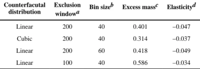
Table 1 shows the results of implementing this approach. The bunching estimate B is calculated as the number of people who are empirically around the kink (Nactual) over and above the number of people who we (counterfactually) estimate would be in this area if the
A
uthor Man
uscr
ipt
A
uthor Man
uscr
ipt
A
uthor Man
uscr
ipt
A
uthor Man
uscr
ipt
kink did not exist (Ncounter); in other words, B = Nactual − Ncounter. The different rows of Table 1 report results under different approaches to approximating that counterfactual distribution of spending that would exist in the absence of the kink, and different definitions of what it means to be “around” the kink. The first three columns describe the approach. The fourth column reports the excess mass, which is the ratio of B to the (counterfactual) number of individuals that would be near the kink in the absence of a kink; in other words, the excess mass is defined as (Nactual − Ncounter)/Ncounter. The final column of Table 1 reports our elasticity estimate. We compute plan-specific α’s using equation 7, our estimate of B for each plan, and plan-specific values for c0 and c1. As noted, our specification implies a constant elasticity α of spending with respect to (2−c). We therefore map our estimates of α to an individual-specific spending elasticity with respect to the (ex-post) individual-specific end-of-year coinsurance rate c; this corresponds to the relevant price the individual responds to in the Saez-style static model with perfect foresight. We report the average elasticity estimate across the individuals in our sample.
The first row of Table 1 shows our baseline specification. We approximate the counterfactual distribution of spending that would exist near the kink if there was no kink by fitting a linear approximation to the cdf, using only individuals in $40 spending bins whose spending is below the kink (between $2,000 and $200 from the kink), and subject to an integration constraint, which requires the overall number of individuals within $2,000 of the kink (in both directions) to remain the same, as in the actual data. We then use a $200 window around the kink to produce our bunching estimate B. The other rows of Table 1 show the sensitivity of our elasticity estimate to fitting a cubic approximation (second row), changing the spending bin size (third row), or changing the size of the exclusion window around the kink (bottom row). These exercises produce relatively similar – and quite small – elasticity estimates, ranging from −0.034 to −0.049.
3.2. The dynamic model from Einav, Finkelstein, and Schrimpf (2015)
An alternative model that one could use to map the bunching pattern to an underlying elasticity of spending with respect to the contract is the one we developed and used in our earlier work on the topic, in Einav, Finkelstein, and Schrimpf (2015). We consider a risk-neutral, forward looking individual who faces stochastic health shocks within the coverage period; at the beginning of the coverage period (a year), an individual faces uncertainty regarding the distribution of health shocks she will face, and makes prescription drug purchase decisions sequentially as information gradually unfolds.2 These health shocks can be treated by filling a prescription. The individual is covered by a non-linear prescription drug insurance contract j over an annual coverage period of T = 52 weeks. A coverage contract is given by a function C(θ, x), which specifies the out-of-pocket amount c the individual would be charged for a prescription drug that costs θ dollars, given total (insurer plus out-of-pocket) spending of x dollars up until that point in the coverage period.
2The assumption of risk neutrality may seem odd in the context of insurance. Note however we are focused not on insurance demand but on the demand for drugs conditional on the insurance contract. Conceptually, risk neutrality may not be a bad approximation for week-to-week decision making, even when the utility function over annual quantities (of income and/or health) is concave. Practically, we showed in Einav, Finkelstein and Schrimpf (2015) that our quantitative results were robust to an alternative model which allowed for risk aversion, at the cost of some expositional and estimation complexity.
A
uthor Man
uscr
ipt
A
uthor Man
uscr
ipt
A
uthor Man
uscr
ipt
A
uthor Man
uscr
ipt
The individual’s utility is linear and additive in health and residual income. Health events are given by a pair (θ, ω), where θ > 0 denotes the dollar cost of the prescription and ω > 0 denotes the (monetized) health consequences of not filling the prescription. We assume that individuals make a binary choice whether to fill the prescription, and a prescription that is not filled has a cumulative, additively separable effect on health. Thus, conditional on a health event (θ, ω), the individual’s flow utility is given by
(8)
When health events arrive they are drawn independently from a distribution G(θ, ω). It is also convenient to define G(θ, ω) ≡ G2(ω|θ)G1(θ). Health events arrive with a weekly probability λ′, which is drawn from H(λ′|λ) where λ is the weekly arrival probability from the previous week. We allow for serial correlation in health by assuming that λ′ follows a Markov process, and that H(λ′|λ) is (weakly) monotone in λ in a first order stochastic dominance sense.
The only choice individuals make is whether to fill each prescription. Optimal behavior can be characterized by a simple finite horizon dynamic problem. The three state variables are the number of weeks left until the end of the coverage period, which we denote by t, the total amount spent so far, denoted by x, and the health state, summarized by λ, which denotes the event arrival probability in the previous week.
The value function υ(x, t, λ) represents the present discounted value of expected utility along the optimal path and is given by the solution to the following Bellman equation:
(9)
with terminal conditions υ(x, 0, λ) = 0 for all x. Optimal behavior is straightforward to characterize: if a prescription arrives, the individual fills it if the value from doing so, −C(θ, x)+δυ(x+θ, t−1, λ′), exceeds the value obtained from not filling the prescription, −ω +
δυ(x, t − 1, λ′).
Estimation and implied elasticities—To estimate the model, we parameterize the key objects. We assume that G1(θ) is lognormal. We assume that G2(ω|θ) follows a mixture distribution with ω = θ with probability 1−p, and ω is drawn from a uniform distribution over [0, θ] with probability p. We allow heterogeneity across individuals assuming that they are drawn from five latent types, and almost all parameters (with the main exception of δ) are type-specific.
A
uthor Man
uscr
ipt
A
uthor Man
uscr
ipt
A
uthor Man
uscr
ipt
A
uthor Man
uscr
ipt
We then estimate the model using simulated moments, where the two key moments we use are the bunching pattern presented in Figure 3 and the differential pattern of monthly claim propensities for individuals that are close and far from the kink. Specifically, in addition to the bunching moments that are the focus of the current paper, we construct 12 timing moments: for each month from July to December, we match the share of individuals with at least one claim in the month conditional on the individuals total spending in the year being within $150 of the kink, and an analogous share conditional on the individuals’ total spending being between $800 and $500 below the kink. As one more way to capture the dynamic aspect of the problem, we also use as a moment the covariance between
individuals’ spending in the first half and second half of the year, which is informative about the persistence of spending over time.
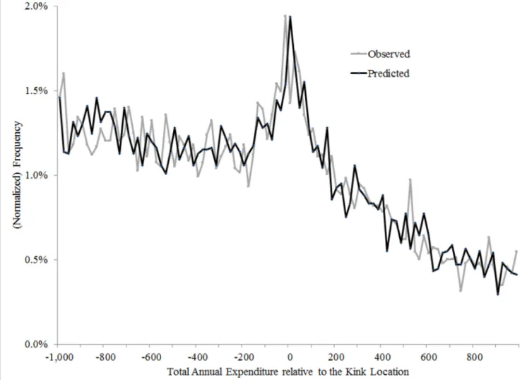
This is all, by design, identical to the model and estimation carried in Einav, Finkelstein, and Schrimpf (2015), which provide much more details about the parameterization and
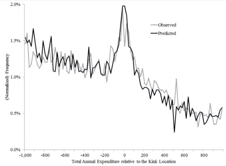
estimation. The results are also similar, but not exactly the same because of the additional sample restrictions. Figure 4 shows the fit of the model to the bunching patterns; by design, the fit is quite close. Appendix Table A1 present the parameter estimates.
Using the model and its estimates, we can now perform counterfactual exercises regarding changes in the budget set. Given our focus on generating estimates that are comparable to the Saez-based elasticity estimates obtained in the last section, our main exercise relies on applying a uniform percentage price reduction to the budget sets (analogous to the one presented in Figure 1) of the contracts that in our sample. We then simulate spending decisions for each individual under his original coverage plan and under the modified plans, and use these to compute elasticities.3
The results are summarized in Table 2. The implied elasticities range from −0.22 to −0.26. These are about five times larger than the implied elasticities from the static model (see Table 1).
4. Understanding the models’ different implications
The previous section established the central “result” of the paper: two different, natural (in our view!) models of spending behavior that are empirically fitted to the bunching or excess mass pattern in Figure 3 produce quantitatively very different implications for the underlying economic object of interest one might want to use out of sample. The models are not similar, yet they use the same key source of variation, so one might have expected them to produce elasticity estimates of similar magnitudes. However, comparing the results in Table 1 and Table 2 suggest that the Saez-based elasticity estimates (Table 1) are about five times lower than the dynamics-based elasticity estimates (Table 2). This raises a natural question: why? In this section we briefly explore – conceptually and empirically – which economic and modeling assumptions seem to be important in creating the different quantitative
3As emphasized by Aron-Dine, Einav, and Finkelstein (2013) and Aron-Dine et al. (2015), if individuals face a non-linear budget set and take the dynamic incentives it creates into account, it is not advisable to characterize the elasticity of spending with respect to “the price” without specifying the complete price change along the entire non-linear budget set.
A
uthor Man
uscr
ipt
A
uthor Man
uscr
ipt
A
uthor Man
uscr
ipt
A
uthor Man
uscr
ipt
implications. A simple, clear statement of what is driving the different results will not be easy; the models are not nested versions of each other. Nor, it is worth emphasizing, do we consider them vertically rankable in terms of their appeal. The static, frictionless model à-la Saez (2010) has the attraction of being a simple and transparent mapping from a descriptive fact to an economic object of interest; relatedly, it can be implemented easily and quickly. The dynamic model is more computationally challenging and time consuming to implement and – not unrelatedly – a bit more of a “black box” in terms of the relationship between the underlying data objects and the economic object of interest. As we now discuss, these disamenities are introduced in order to account for three potentially important economic forces in our context that our adaptation of Saez’s static, frictionless model abstracts from: lumpiness in drug purchases, uncertainty, and discounting. We sometimes refer to the latter two under the general rubric of “dynamics,” although they are conceptually somewhat distinct.
4.1. Conceptual differences
A first distinction between the two approaches regards frictions. The adaptation to the Saez model assumes away any frictions (including lumpiness). This is arguably a more important restriction in the context for which it was originally developed – labor supply decisions. As has been discussed extensively (Chetty, 2012; Chetty et al., 2011, 2013a, 2013b; Bastani and Selin, 2014), labor supply decisions are likely restricted to certain discrete choices (e.g., full time or part time), which will by necessity limit the amount of bunching at the kink that a given underlying behavioral response can produce. Practical implementations of Saez (2010) allow for some frictions – by measuring bunching in some bandwidth around the kink rather than simply a spike at the kink which is the literal implication of the frictionless model – but will still miss any behavioral response to the kink that does not result in an outcome within that bandwidth. Such lumpiness is arguably less important in our setting, where a typical prescription drug costs $20 (for generic drugs) or $130 (for branded drugs), which is only a small fraction of total annual spending for those individuals whose spending is around the kink. Yet, this is still potentially a force that would reduce the implied behavioral elasticity estimated in the Saez-style approach, since any lumpiness will work to push spending outside of the bandwidth used to measure excess mass. The dynamic model, by contrast, accounts for lumpiness by modeling a discrete series of (weekly) health shocks and purchase decisions, explicitly estimating the distribution of the cost of each drug (θ), whose right tail is not trivial.
Second, the Saez model is a static model. This seems a reasonable approximation to many annual labor supply decisions, which was the context for which it was developed.5 However, a static model seems poorly suited to our context. Annual spending in our setting is the result of individuals making many sequential prescription drug purchase decisions throughout the year as health shocks arrive (and information is revealed), and the price of treating each shock changes as individuals move along their non-linear budget set. This is in sharp contrast to the assumption of the static framework in which all the uncertainty is realized prior to any spending decision.
A
uthor Man
uscr
ipt
A
uthor Man
uscr
ipt
A
uthor Man
uscr
ipt
A
uthor Man
uscr
ipt
Relatedly, if individuals respond to the dynamic incentives provided by the non-linear contract, then not only does information arrive gradually, but also early purchase decisions reflect individuals’ expectations about future health shocks and their associated out-of-pocket price, adding yet another important dynamic effect. For example, the static analysis, by construction, limits the behavioral response to the kink to those near the kink. Yet, the set of people “near” the kink – and therefore “at risk” of bunching – may in fact be
endogenously affected by the presence of the kink; forward-looking individuals, anticipating the increase in price if they experience a series of negative health shocks, are likely to make purchase decisions that decrease their chance of ending up near the kink, even if at that point they are far from reaching it.
This is not merely a theoretical point. In prior empirical work, we produced reduced form, descriptive evidence that is consistent with such forward looking behavior; in particular, in both prescription drug purchasing in Medicare Part D and in medical spending decisions in employer-sponsored health insurance we presented evidence that individuals. health care utilization decisions respond to the future price of health care (Aron-Dine et al., 2015). Specifically, in both settings, we found that individuals in the same health insurance contract who face the same spot price of healthcare but a higher expected end-of-year price of care (because they joined the non-linear contract at different points during the year) have lower initial healthcare spending. This evidence of a response to the future price of care, among individuals who face the same spot, or initial price of care, is consistent with individuals taking into account the entire non-linear budget set in making current healthcare utilization choices.
Relatedly, our prior estimates of the dynamic model described in the previous section found a non-trivial role for such “anticipatory” behavioral responses by people who expected to end up far below the kink; for example, we estimated that about a quarter of the spending increase that we project will occur from “filling the donut hole” in Medicare Part D is associated with beneficiaries whose spending prior to the policy change would leave them short of reaching the donut hole (Einav, Finkelstein, and Schrimpf, 2015). Any such anticipatory response to the donut hole (or any non-linear feature of the health insurance contract), will be mechanically missed by a Saez-style “bunching” estimator since, by definition, this behavioral response does not happen around the kink.
Thus, qualitatively, both the assumption of a frictionless environment and the assumption of a static environment seem likely to contribute to the lower Saez-based elasticity in Table 1 compared to the dynamics-based elasticity in Table 2. We now endeavor to explore the quantitative importance of each factor by estimating various restricted versions of the “full” dynamic model that shut down various features. Of course, these various modeling features are unlikely to have an additively separable effect on the estimates. so it will not be possible to do a strict accounting-style decomposition of the contribution of frictions vs. static modeling to the differences between the two estimates.
Relatedly, an important point to keep in mind in any such exercise is that if we re-estimate the “restricted” models, all of the parameter estimates will change in an attempt to have the restricted models fit the various moments in the data (including the bunching at the kink) as
A
uthor Man
uscr
ipt
A
uthor Man
uscr
ipt
A
uthor Man
uscr
ipt
A
uthor Man
uscr
ipt
well as possible. In other words, this exercise is different from a theoretical comparative statics exercise. This is because the data, and in particular the bunching pattern, is held fixed, and is being fitted by any of the models we propose, so as we move from one specification to another, the parameters are re-estimated and change in response to modeling restrictions. As a result, a comparison of implied elasticities from various alternative models – each separately estimated to fit the data – may not lead to intuitive (or conceptually interesting) comparative statics.
4.2. Quantitative differences
We consider two “restricted” versions of the “full” dynamic model presented earlier. These versions are designed to shut down various features that are absent from the Saez-style model. In the first – which we refer to as Restricted Model A (“no dynamics”) – we restrict the full model to shut down dynamics. Specifically, we start with the full model and its parameterization, but then assume no discounting or uncertainty as in Saez (2010). Yet, we continue to allow for frictions in the form of lumpy spending. To do so, consider the dynamic model from the previous section, but assume that individuals. discount factor is δ = 1 and that they do not face any uncertainty regarding the future. That is, as of the first week of the year individuals have complete information about the precise set of health events that they would experience throughout the year.
These assumptions make the individual drug expenditure decision a static problem. To see this, let denote the set of health events realized during the coverage year, with (θt, ωt) = (0, 0) if there was no health event at week t, and it is easy to see that the individual optimal decision is simply a linear programming problem of choosing the subset D ⊆ H of the prescriptions that get filled. The individual will choose D to solve the following problem:
(10)
which is conceptually very similar to the individual problem of maximizing equation (2) in the Saez-style model in Section 3. A key difference between our static version of the dynamic model and the Saez-style model is that the former allows for the lumpiness of claims, relative to the frictionless spending model of Saez (of course, there are also unavoidable functional form differences between the two). In particular, given 52 weeks in the year and an estimated average weekly arrival rate of a health shock of approximately 0.4 (see the estimates of λ in Appendix Table A1), the typical individuals faces about 20 shocks, so a relatively finite set of choices of which to make claims (some of which will have θ > ω and therefore are effectively non-discretionary).
In the second restricted model – which we refer to as Restricted Model B (“no discounting”) – we impose δ = 1 on the full model, rather than allowing δ to be a free estimable parameter. It thus allows for lumpiness of spending, as in the first restricted model, but also allows for uncertainty in the timing and nature of health shocks throughout the year. By imposing δ =
A
uthor Man
uscr
ipt
A
uthor Man
uscr
ipt
A
uthor Man
uscr
ipt
A
uthor Man
uscr
ipt
1, all the dynamic behavior is due to uncertainty and incomplete information about the future, rather than due to time preferences.
Both of these restricted models use a similar basic structure to that of the full model presented in the previous section. We thus follow the same econometric and parametric assumptions regarding functional form, distributions, and heterogeneity, and use the same method of simulated moments and the same set of empirical moments for estimation. We should note, however, that the combination of lumpiness and complete information in Restricted Model A leads to a computational problem: although conceptually trivial, solving the optimization problem in equation (10) is in fact complicated as it leads to a large combinatorial choice. Therefore, to estimate Restricted Model A we use approximation techniques, as detailed in the appendix.
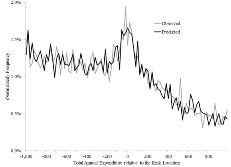
In the appendix (Appendix Table A2 and Appendix Table A3), we report the underlying parameter estimates that are associated with each model. Loosely, the parameter estimates are reasonably similar across models. This is not particularly surprising given how similar the models are, and the fact that they try to fit the same descriptive (bunching) patterns in the data. Indeed, like the full dynamic model and the Saez-style model, these two restricted models also fit the bunching pattern well as we show in Figure 5 and Figure 6. Yet, it is interesting to discuss the parameter that have changed as we move from the full dynamic model to restricted models A and B. Those changing parameters are those that “compensate” for the changes in the modeling assumptions, and may provide some intuition for why the elasticity estimates change. For example, comparing the estimates for model A (Appendix Table A2) with the estimates of the full model (Appendix Table A1) reveals that imposing certainty makes us estimate health shocks that are slightly more persistent, and most importantly make us estimate lower moral hazard parameter p for the two high-spending types, and this latter differences is presumably what drives the lower price elasticity implied by the certainty model.
The key focus is the implications of these different models – all of which are designed to fit the bunching pattern – for the economic object of interest: the elasticity of annual spending with respect to the out-of-pocket price. The main results are presented in Table 3 Panel A shows the results for Restricted Model A (“no dynamics”) and panel B for Restricted Model B (“no discounting”). Each table reports the implied elasticities in a parallel fashion to the way Table 2 was generated for the “full” dynamic model of Section 3. Recall that the Saez-style model predicted Saez-based elasticity estimates in the range of −0.04 to −0.05 (Table 1) while the “full” dynamic model produced dynamics-based estimates of −0.22 to −0.26 (Table 2). For ease of discussion we focus on the midpoint of this range, looking at a 15 percent reduction in price in Tables 2 and 3.
The “full” dynamic model generates an “elasticity” with respect to the 15 percent price reduction of −0.25 (Table 2) while the “no dynamics” model in Panel A of Table 3 generates an elasticity of −0.13. This “no dynamics” model represents our attempt to approximate – within our more richly parametrized model – a static model à-la Saez. A key difference between the “no dynamics” model and the Saez-style model is that the latter, as discussed, is frictionless, whereas the “no dynamics” model allows for lumpiness in drug purchases.
A
uthor Man
uscr
ipt
A
uthor Man
uscr
ipt
A
uthor Man
uscr
ipt
A
uthor Man
uscr
ipt
Thus, one way to interpret these results is that lumpiness in purchases may explain about half of the difference in elasticity estimates between the two models. Of course, there are functional form differences between the “no dynamics” model and the Saez-style model which may also impact the results.
As noted, the “no dynamics” model shuts down both discounting and uncertainty. Panel B of Table 3 explores the importance of discounting by estimating a version of the full model that allows for uncertainty but imposes no discounting (δ = 1). As it turns out, the assumption regarding the discount factor do not have a major effect on the implied elasticity. The “no discounting” model in Panel B of Table 3 yields an elasticity (for a 15 percent price reduction) of −0.22, which is quite close to the “full model” estimate of −0.25 (relative to the “no dynamics” estimate of −0.13). In other words, after lumpiness, allowing for dynamics in the form of uncertainty appears important for the elasticity estimate, but discounting per se does not (although could be important for other objects of interest). We close by re-emphasizing our earlier caveat that comparisons across the “full” dynamic model and the various restricted models are not “real” comparative statics. In each case, the model was re-estimated and the parameters changed (see Appendix Tables A1 through A3) as the restricted models also tried to match the (observed) bunching moments. As a result, it is hard to develop economic intuition for “why” the restricted models deliver the results that they do relative to the full model. In practice, in our setting we found that the “real”
comparative statics generate much smaller changes in elasticities than the re-estimated restricted models. For example, if we take the parameter estimates from the full model (Table A1) but impose the restrictions of the “no discounting” model (i.e. we impose δ = 1), we estimate that the elasticity declines from −0.25 to −0.23, which is only two-thirds as much as the decline if we instead re-estimate the model after imposing no discounting (in which case, we estimate an elasticity of −0.22). Similarly, if we take the parameter estimates from the full model but impose the restrictions of the “no dynamics” model (i.e. assume perfect foresight of the sequence of health events, and assume δ = 1), we estimate that the elasticity declines from −0.25 to −0.20, which less than a half of the decline if we instead re-estimate the model (in which case, we re-estimate an elasticity of −0.13).
5. Conclusions
This paper documents a case in which two different models both fit well in sample, but have different implications out of sample. We illustrated this point in the specific context of translating bunching estimates – which are being increasingly used in public economics – to behavioral elasticities, and in the specific setting of studying the spending (or “moral hazard”) effects of health insurance contracts. We showed that the translation of a descriptive bunching pattern to an elasticity estimate using a Saez-style frictionless model could lead to five-fold lower counterfactual predictions relative to those generated by a richer dynamic model. While this qualitative result – that two different models lead to different results – by itself should be hardly surprising, we did not expect a-priori such a large difference in the magnitude of the prediction. We explored several “in-between” specifications to help assess which modelling assumptions may be most responsible for the differences in results.
A
uthor Man
uscr
ipt
A
uthor Man
uscr
ipt
A
uthor Man
uscr
ipt
A
uthor Man
uscr
ipt
Given these results, an obvious question is how to select among the many models that could rationalize an observed pattern. There is of course no algorithmic answer to this question, and model selection should likely depend on the context, the data at hand, and the key counterfactual exercise for which it is used. Additional moments and external information could help with model selection. Other aspects that could factor into such a decision are tradeoffs between transparency, simplicity, and speed of communication on the one hand, and richness of the model on the other hand. When there is enough reason (or evidence) to believe that a richer model could lead to substantially different results, it seems more important to move away from the simpler model.
However, we should note that even when simpler models are inferior in terms of a bottom-line counterfactual, they may still prove quite useful in other respects. For example, going back to the specific application of the current paper, even though the Saez-style model delivers elasticities that are much lower, it may generate useful qualitative results regarding elasticity differences across groups. It can provide a relatively easy and quick way for general testing and assessment before developing and estimating more complete models. The exercise in our paper is a specific illustration of a broader challenge facing applied work. There is a growing premium on compelling, transparent, “reduced form” evidence of a behavioral response. At the same time, there is growing appreciation of the observation that translation of that reduced form evidence into an economic object of interest often requires additional modeling assumptions and data moments. The “bunching” literature – which has focused on visually compelling evidence of behavioral responses – has been particularly attuned to this issue, and developed several modeling approaches, as summarized in Kleven (2016). While our paper fits squarely in that “bunching” literature, the challenge is of course much broader, and applies to any attempt to translate reduced form evidence of a behavioral response – be it the excess mass at a convex kink or a treatment effects from a randomized controlled trial – into an underlying economic object.
Acknowledgments
Einav and Finkelstein gratefully acknowledge support from the NIA (R01 AG032449). We thank John Friedman, Henrik Kleven, Matthew J. Notowidigdo, Wojciech Kopczuk, Whitney Newey, and an anonymous referee for helpful comments.
References
Abaluck, J., Gruber, J., Swanson, A. Prescription drug use under Medicare part D: A linear model of nonlinear budget sets; NBER Work. Pap. 20976; 2015.
Aron-Dine A, Einav L, Finkelstein A. The RAND health insurance experiment, three decades later. J. Econ. Perspectives. 2013; 27(1):197–222.
Aron-Dine A, Einav L, Finkelstein A, Cullen M. Moral hazard in health insurance: do dynamic incentives matter? Rev. Econ. Statistics. 2015; 97(4):725–741.
Bajari, P., Hong, H., Park, M., Town, R. Estimating price sensitivity of economic agents using discontinuity in nonlinear contracts. Mimeo, UC Berkeley: 2016. http://faculty.haas.berkeley.edu/ mpark/NonlinearContract.pdf
Bastani S, Selin H. Bunching and non-bunching at kink points of the Swedish tax schedule. J. Public Econ. 2014; 109(C):36–49.
A
uthor Man
uscr
ipt
A
uthor Man
uscr
ipt
A
uthor Man
uscr
ipt
A
uthor Man
uscr
ipt
Best, MC., Kleven, H. Housing market responses to transaction taxes: evidence from notches and
stimulus in the UK. Mimeo: London School of Economics; 2016. http://www.henrikkleven.com/
uploads/3/7/3/1/37310663/best-kleven_landnotches_feb2016.pdf
Best, MC., Cloyne, J., Iltzetzki, E., Kleven, H. Interest rates, debt and intertemporal allocation: evidence from notched mortgage contracts in the UK. Mimeo: London School of Economics; 2015.
http://www.henrikkleven.com/uploads/3/7/3/1/37310663/best-cloyne-ilzetzki-kleven_aug2015.pdf
Blomquist, S., Kumar, A., Liang, CY., Newey, WK. Individual heterogeneity, nonlinear budget sets, and taxable income; CESifo Working Paper No. 5320; 2015.
Chetty R. Sufficient statistics for welfare analysis: a bridge between structural and reduced-form methods. Ann. Rev. Econ. 2009; 1:451–488.
Chetty, R., Friedman, JN., Olsen, T., Pistaferri, L. Adjustment costs, firm responses, and micro vs. macro labor supply elasticities: Evidence from Danish tax records; NBER Work. Pap. 15617; 2009.
Chetty R, Friedman JN, Olsen T, Pistaferri L. Adjustment costs, firm responses, and micro vs. macro labor supply elasticities: Evidence from Danish tax records. Quart. J. Econ. 2011; 126(2):749–804. Chetty R. Bounds on elasticities with optimization frictions: A synthesis of micro and macro evidence
on labor supply. Econometrica. 2012; 80(3):969–1018.
Chetty R, Friedman JN, Saez E. Using differences in knowledge across neighbor-hoods to uncover the impacts of the EITC on earnings. Am. Econ. Rev. 2013a; 103(7):2683–2721.
Chetty R, Guren A, Manoli D, Weber A. Does indivisible labor explain the difference between micro and macro elasticities? a meta-analysis of extensive margin rlasticities. NBER Macroeconomics Annual. 2013b; 27:1–56.
Dalton C, Gowrisankaran G, Town R. Myopia and complex dynamic incentives: evidence from Medicare part D. NBER Work. Pap. 21104. 2015
Einav L, Finkelstein A, Ryan S, Schrimpf P, Cullen M. Selection on moral hazard in health insurance. Am. Econ. Rev. 2013; 103(1):178–219. [PubMed: 24748682]
Einav L, Finkelstein A, Schrimpf P. The response of drug expenditure to nonlinear contract design: Evidence from Medicare part D. Quart. J. Econ. 2015; 130(2):841–899.
Grubb M. Consumer inattention and bill-shock regulation. Rev. Econ. Stud. 2015; 82(1):219–257. Grubb M, Osborne M. Cellular service demand: biased beliefs, learning, and bill shock. Am. Econ.
Rev. 2015; 105(1):234–271.
Ito K. Do consumers respond to marginal or average price? evidence from nonlinear electricity pricing. Am. Econ. Rev. 2014; 104(2):537–563.
Kleven H. Bunching. Ann. Rev. Econ. 2016; 8:435–464.
Kleven H, Knudsen M, Kreiner C, Pedersen S, Saez E. Unwilling or unable to cheat? evidence from a tax audit experiment in Denmark. Econometrica. 2011; 79(3):651–692.
Kleven H, Landais C, Saez E, Schultz E. Migration and wage effects of taxing top earners: evidence from the foreigners’ tax scheme in Denmark. Quart. J. Econ. 2014; 129(1):333–378.
Kleven H, Waseem M. Using notches to uncover optimization frictions and structural elasticities: theory and evidence from Pakistan. Quart. J. Econ. 2013; 128(2):669–723.
Kopczuk W, Munroe D. Mansion tax: the effect of transfer taxes on the residential real estate market. Am. Econ. J.: Econ. Policy. 2015; 7(2):214–257.
Manoli DS, Weber A. Nonparametric evidence on the effects of financial incentives on retirement decisions. Am. Econ. J.: Econ. Policy. forthcoming.
Nevo A, Turner JL, Williams JW. Usage-based pricing and demand for residential broadband. Econometrica. 2016; 84(2):411–443.
Saez, E. Do taxpayers bunch at kink points?; National Bureau of Economic Research Working Paper No. 7366; 1999.
Saez E. Do taxpayers bunch at kink points? Am. Econ. J.: Econ. Policy. 2010; 2(3):180–212. Sallee JM, Slemrod J. Car notches: strategic automaker responses to fuel economy policy. J. Public
Econ. 2012; 96(11):981–999.
A
uthor Man
uscr
ipt
A
uthor Man
uscr
ipt
A
uthor Man
uscr
ipt
A
uthor Man
uscr
ipt
Appendix
In this appendix we describe the approximation we use to Restricted Model A in the paper. That is, the version of the model that has no uncertainty (and therefore no dynamics). With full certainty, a consumer faces a collection of potential prescriptions and must choose which ones to fill. Denote dt = 1 if a prescription is filled and dt = 0 if not. The consumer’s problem is
(A1)
It is very difficult to solve this discrete optimization problem. There are 252 possible sequences of dt, so a brute force solution is computationally intractable. The dynamic programming approach that we used in the model with uncertainty is also not applicable here. With uncertainty, spending until time t and the current ωt and θt are the relevant state variables for a consumer. With certainty, the consumer knows the entire sequence of θt and
ωt, so this entire sequence is relevant for the consumer’s decision at time t.
To make computation tractable, we exploit the fact that the budget, C(·), is piecewise linear, impose δ = 1, and settle for an approximate solution when the exact solution lies near the convex kink. Given that the budget is piecewise linear, we can write it as
(A2)
where kg are increasing with g. Once restricted to lie on a given segment of the budget set, the consumer’s problem is an integer linear program,
(A3)
Although there are algorithms to solve integer linear programs, integer linear programs are NP hard, so the performance of these algorithms can be poor. Using them in our context was too time consuming; we must solve the above problem thousands of times to estimate the model. Instead, we compute an approximate solution as follows. Consider the relaxation of (A3) to a linear program by allowing dt to take any value in the interval [0, 1] (instead of either 0 or 1, as in the original problem):
A
uthor Man
uscr
ipt
A
uthor Man
uscr
ipt
A
uthor Man
uscr
ipt
A
uthor Man
uscr
ipt
(A4)
There are three possible solutions. Two corner solutions and an interior one,
(A5)
Note that the interior solution has all dt∈ {0, 1}, so if the solution is interior, then the solution is the same with or without the integer constraint. To describe the upper corner solution, sort prescriptions such that
(A6)
Let . Then dt(r) = 1 for r < r*, 0 for r > r* and
(A7)
The solution is very intuitive and simple. We sort potential prescriptions by their relative cost of not filling, , and then fill from most costly to least costly until we reach the corner. Unfortunately, the corner solution violates the integer constraint. Simply rounding the solution to the not-integer-constrained linear program does not necessarily give the solution to the integer constrained linear program. Nonetheless, we adapt the rounded solution as an approximate optimum.
After (approximately) solving the model along each segment, we take the segment solution that gives the highest utility as the solution. Note that the only time an approximate corner solution will be used is if the solution is at the single convex kink. Also, in these cases, the true and approximate solutions both have the feature that either switching a single
prescription from filled to not filled (or vice versa) would move total spending from above to below the convex kink. The solution is only approximate in that there may be a better set of prescriptions to fill with this feature.
A
uthor Man
uscr
ipt
A
uthor Man
uscr
ipt
A
uthor Man
uscr
ipt
A
uthor Man
uscr
ipt
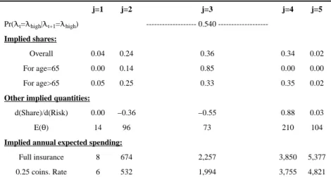
Appendix Table A1
Parameter estimates from the dynamic model
j=1 j=2 j=3 j=4 j=5 Parameter estimates: Beta_0 0.00 3.60 4.02 −4.37 −4.39 Beta_Risk 0.00 −2.44 −2.81 4.09 6.17 Beta_65 0.00 −0.13 1.35 0.93 −1.59 δ 0.97 ---μ 0.013 3.96 2.93 4.38 4.35 σ 2.35 1.14 1.57 0.43 1.42 p 0.86 0.91 0.52 0.51 0.44 λlow 0.013 0.15 0.65 0.86 0.47 λhigh 0.011 0.13 0.57 0.75 0.41 Pr(λt=λlow|λt+1=λlow) 0.557 ---Pr(λt=λhigh|λt+1=λhigh) 0.565 ---Implied shares: Overall 0.05 0.27 0.34 0.03 0.31 For age=65 0.00 0.13 0.87 0.00 0.00 For age>65 0.05 0.27 0.32 0.03 0.33
Other implied quantities:
d(Share)/d(Risk) 0.00 −0.37 −0.52 0.06 0.83 E(θ) 16 101 65 87 211
Implied annual expected spending:
Full insurance 11 811 2,198 3,891 5,110 0.25 coins. Rate 8 627 1,914 3,398 4,542
Top panel reports parameter point estimates (standard errors are available from the authors upon request) from the dynamic model of Einav, Finkelstein, and Schrimpf (2015). Bottom panels report implied quantities based on these parameters.
Appendix Table A2
Parameter estimates from restricted model A (“no dynamics”)
j=1 j=2 j=3 j=4 j=5 Parameter estimates: Beta_0 0.00 3.56 4.03 −4.29 −4.66 Beta_Risk 0.00 −2.39 −2.63 6.37 4.10 Beta_65 0.00 0.01 1.34 −1.61 0.85 δ 1.00 (Imposed) ---μ 0.043 3.98 2.95 4.34 4.52 σ 2.29 1.08 1.64 1.42 0.51 p 0.82 0.84 0.47 0.10 0.41 λlow 0.010 0.14 0.60 0.35 0.99 λhigh 0.008 0.10 0.46 0.27 0.77 Pr(λt=λlow|λt+1=λlow) 0.611
---A
uthor Man
uscr
ipt
A
uthor Man
uscr
ipt
A
uthor Man
uscr
ipt
A
uthor Man
uscr
ipt
j=1 j=2 j=3 j=4 j=5 Pr(λt=λhigh|λt+1=λhigh) 0.540 ---Implied shares: Overall 0.04 0.24 0.36 0.34 0.02 For age=65 0.00 0.14 0.85 0.00 0.00 For age>65 0.05 0.25 0.33 0.35 0.02
Other implied quantities:
d(Share)/d(Risk) 0.00 −0.36 −0.55 0.88 0.03
E(θ) 14 96 73 210 104
Implied annual expected spending:
Full insurance 8 674 2,257 3,850 5,377 0.25 coins. Rate 6 532 1,994 3,755 4,821
Table reports estimation results from restricted model A (“no dynamics”), which is described in the main text. Table structure parallels that of Appendix Table A1.
Appendix Table A3
Parameter estimates from restricted model B (“no discounting”)
j=1 j=2 j=3 j=4 j=5 Parameter estimates: Beta_0 0.00 3.63 4.01 −4.28 −4.36 Beta_Risk 0.00 −2.49 −2.85 4.07 6.27 Beta_65 0.00 −0.07 1.28 0.97 −1.65 δ 1.00 (Imposed) ---μ −0.015 4.02 2.94 4.43 4.32 σ 2.34 1.24 1.55 0.32 1.39 p 0.86 0.96 0.46 0.49 0.39 λlow 0.012 0.14 0.63 0.90 0.49 λhigh 0.010 0.12 0.52 0.75 0.41 Pr(λt=λlow|λt+1=λlow) 0.570 ---Pr(λt=λhigh|λt+1=λhigh) 0.568 ---Implied shares: Overall 0.05 0.26 0.33 0.03 0.33 For age=65 0.00 0.15 0.85 0.00 0.00 For age>65 0.05 0.27 0.31 0.03 0.34
Other implied quantities:
d(Share)/d(Risk) 0.00 −0.39 −0.52 0.05 0.86 E(θ) 15 120 62 89 196
Implied annual expected spending:
Full insurance 9 891 2,038 4,137 5,018 0.25 coins. Rate 7 678 1,804 3,626 4,529
Table reports estimation results from restricted model B (“no discounting”), which is described in the main text. Table structure parallels that of Appendix Table A1.
A
uthor Man
uscr
ipt
A
uthor Man
uscr
ipt
A
uthor Man
uscr
ipt
A
uthor Man
uscr
ipt
Figure 1. Medicare Part D standard benefit design (in 2008)
The figure shows the standard benefit design in 2008. “Pre-Kink coverage” refers to coverage prior to the Initial Coverage Limit (ICL) which is where there is a kink in the budget set and the gap, or donut hole, begins. The level at which catastrophic coverage kicks in is defined in terms of out-of-pocket spending (of $4,050), which we convert to the total expenditure amount provided in the figure. Once catastrophic coverage kicks in, the actual standard coverage specifies a set of co-pays (dollar amounts) for particular types of drugs; in the figure we use show a 7% insurance rate, which is the empirical average of these co-pays in our data.
A
uthor Man
uscr
ipt
A
uthor Man
uscr
ipt
A
uthor Man
uscr
ipt
A
uthor Man
uscr
ipt
Figure 2. Rationale for bunching
The solid line illustrates the budget set of the same standard benefit design as in Figure 1. The dashed line considers an alternative budget set with a linear budget (above the
deductible) at the co-insurance arm’s cost sharing rate. By contrast, the standard budget set has a kink (price increase) at $2,510 in total spending. The individual denoted by the solid indifference curve is not affected by the introduction of this kink; his indifference curve remains tangent to the lower part of the budget set. The individual with the dashed indifference curves consumed above the kink under the linear budget set; with the
introduction of the kink her utility is lower, and her indifference curve is now tangent to the steeper part of the budget set at the kink. With the introduction of the kink, this latter individual would therefore decrease total spending to the level of the kink location. By extension, any individual whose indifference curve was tangent to the linear budget set at a spending level between that of the two individuals shown would likewise decrease total spending to the level of the kink location, thereby creating “bunching” at the kink.