HAL Id: hal-01978686
https://hal.archives-ouvertes.fr/hal-01978686v2
Submitted on 7 May 2020HAL is a multi-disciplinary open access archive for the deposit and dissemination of sci-entific research documents, whether they are pub-lished or not. The documents may come from teaching and research institutions in France or abroad, or from public or private research centers.
L’archive ouverte pluridisciplinaire HAL, est destinée au dépôt et à la diffusion de documents scientifiques de niveau recherche, publiés ou non, émanant des établissements d’enseignement et de recherche français ou étrangers, des laboratoires publics ou privés.
Stability and Reachability analysis for a controlled
heterogeneous population of cells
Cécile Carrère, Hasnaa Zidani
To cite this version:
Cécile Carrère, Hasnaa Zidani. Stability and Reachability analysis for a controlled heterogeneous population of cells. Optimal Control Applications and Methods, Wiley, 2020, 41, pp.1678-1704. �hal-01978686v2�
DOI: xxx/xxxx
ARTICLE TYPE
Stability and Reachability analysis for a controlled heterogeneous
population of cells.
Cécile Carrère
1| Hasnaa Zidani
21Instituto Gulbenkian de Ciência, Fundação
Callouste Gulbenkian, Oeiras, Portugal
2Unité de Mathématiques Appliquées,
ENSTA ParisTech, Saclay, France
Correspondence
Email: [email protected]
This paper is devoted to the study of a controlled population of cells. The modelling of the problem leads to a mathematical formulation of stability and reachability prop-erties of some controlled systems under uncertainties. We use the Hamilton-Jacobi (HJ) approach to address these problems and to design a numerical method that we analyse on several numerical simulations.
KEYWORDS:
Non-linear optimal control; Dynamical programming; Applications to chemotherapy; Reachability anal-ysis
1
INTRODUCTION
The treatment of cancers with cytotoxic chemotherapies often encounters two major pitfalls: the side toxicity of the drugs on healthy cells and organs, and the emergence of resistance to the treatment. This resistance can occur because of an initial genomic heterogeneity of the tumour: in its early stages, it contains several distinct populations of cells, that differ from one another because of successive mutations1. If one of these lineages is resistant to the first line of treatment, then using strong doses of
drug, as it is done in many classical protocols, kills all sensitive cells, and lets this resistant lineage grow without control. It is thus important to take into account cancer heterogeneity before starting a treatment. Mathematical modelling can, in this framework, give guidelines on how to treat such tumours.
For example,2,3study the growth and treatment of heterogeneous tumours, and determine optimal dosages of drugs for fixed
time injections. The treatment protocol is there considered as instantaneous injections of drugs. We will work here in a framework of continous treatment. In4, an ODE model of heterogeneous tumour growth is studied under continuous treatment. The optimal
control theory is used to give necessary conditions on optimal protocols, in order to reduce the tumour volume while preserving its heterogeneity. We refer the reader to5,4,6,7for different models of tumour growth, presented and studied in the framework of
optimal control theory.
In this paper, we will consider a model for heterogeneous tumour growth, with interactions between two cancerous cells populations: 𝑠 which is sensitive to the treatment, and 𝑟 which is resistant to it. The biological model is an in vitro experiment, with both ligneages developping in a Petri dish, so that no other cells intervene in their evolution. It has been already considered in8, where an optimal treatment is characterized to treat heterogeneous tumours. This objective is satisfactory for experiments
on in vitro tumors, but might not be adequate for medical applications with longer time objectives.
The main goal of the present work is to maintain permanently the tumour size under a certain threshold, defined by medical considerations, under which the tumour is considered benign. When this objective cannot be satisfied (for instance, if the initial tumour is already bigger than the designed threshold), we would like to find a good strategy to lower the tumour volume, in such a way that we will then be able to maintain it under the size threshold. These problems will be referred as stability or reachability problems. We will formulate these objectives as control problems that we will solve in the framework of Hamilton-Jacobi (HJ) equations.
An important problem arising from biological applications is the influence of uncertainties. For example, since several cyto-toxic drugs target cells during their dividing phase, the drug efficiency may greatly differ depending on the tumour composition at the time of injection. The Hamilton-Jacobi framework is suitable to consider uncertainties as an opponent player, thus adjusting the optimal strategies to varying parameters.
Hamilton-Jacobi theory has been investigated, for stability and reachability problems, in many works. We refer to9,10,11,12,13,14,15,16and the references therein. In particular, let us also mention the works17where Hamilton-Jacobi framework
is considered to take into account uncertainties in the case of collision avoidance for unmanned vehicles. In that paper, the uncertainty is the trajectory of another vehicle.
Recall that Hamilton-Jacobi equations characterise the value function associated to the control problem. Once this value function is computed numerically, a reconstruction algorithm can be used to get the optimal strategies for stability or for reach-ability. In this paper, we consider a reconstruction algorithm for control problems in presence of state constraints. We prove the convergence of this algorithm and we show with several numerical simulaitons the relevance of our approach.
This article is organized as follows. Section 2 presents the different models, objectives and constraints that will be considered in this paper. Section 3 is devoted to the mathematical analysis. In this section, a Hamilton-Jacobi approach is introduced to characterize some reachability sets. In section 4, we analyse some trajectory reconstruction algorithms. Finally, section 5 presents and analyses some numerical simulations.
2
MATHEMATICAL FORMULATION OF THE PROBLEM
We present here some notations that will be used throughout this paper. We will denote by| ⋅ | the Euclidean norm and by ⟨⋅, ⋅⟩ the Euclidean inner product on ℝ𝑁 (for any 𝑁 ≥ 1). The notation 𝔹 stands for the unit open ball {𝑥 ∈ ℝ𝑁 ∶ |𝑥| < 1} and
𝔹(𝑥, 𝑟) ∶= 𝑥 + 𝑟𝔹 for any 𝑥 ∈ ℝ𝑁 and 𝑟 > 0.
For every set ⊆ ℝ𝑁, ◦
, and 𝜕 denote its interior, closure and boundary, respectively. The distance function to is dist(𝑥,) = inf{|𝑥 − 𝑦| ∶ 𝑦 ∈ }.
For any 𝑀 > 0, the set 𝐿1(0, +∞; 𝑒−𝑀𝑡𝑑𝑡) is the set of functions 𝑓 ∶ [0, +∞) → ℝ such that∫+∞ 0 |𝑓(𝑡)|𝑒
−𝑀𝑡𝑑𝑡is finite:|𝑓|
is integrable for the measure 𝑒−𝑀𝑡𝑑𝑡. The set 𝑊1,1(0, +∞; 𝑒−𝑀𝑡𝑑𝑡) is the set of functions 𝑓 ∈ 𝐿1(0, +∞; 𝑒−𝑀𝑡𝑑𝑡) such that
their derivative is also in 𝐿1(0, +∞; 𝑒−𝑀𝑡𝑑𝑡).
We consider the following controlled differential system :
̇𝑦(𝑡) = 𝑓0(𝑦(𝑡), 𝛼(𝑡)) + 𝑓1(𝑦(𝑡), 𝛼(𝑡))𝑢(𝑡), (1)
where 𝑢 is the control, 𝑦 the vector of state variables (𝑦(𝑡) ∈ ℝ𝑛, with 𝑛 = 2 or 3 depending on the problem we consider), and
𝛼(𝑡) a vector of 𝑚 parameters that can change over time 𝑡, representing the uncertainties. We consider only measurable controls taking value between 0 and a certain 𝑈𝑚𝑎𝑥>0 ; in other words,
𝑢∈ ∶= {𝑢 ∶ ℝ+→ ℝ is measurable, 𝑢(𝑡) ∈ [0, 𝑈𝑚𝑎𝑥] a.e.}.
We also consider that the uncertainties are measurable functions taking values in a given compact subset 𝐴 of ℝ𝑚(with (𝑚≥ 1)): 𝛼∈ ∶= {𝛼 ∶ ℝ+→ ℝ𝑚is measurable, 𝛼(𝑡) ∈ 𝐴 a.e.}
In all the sequel, we will consider models where the vector fields 𝑓0∶ ℝ𝑛× ℝ𝑚 → ℝ𝑛and 𝑓
1 ∶ ℝ𝑛× ℝ𝑚 → ℝ𝑛satisfy the
following assumption:
(𝐇𝐟) 𝑓0and 𝑓1are continuous fonctions, and Lipschitz continuous with respect to the first variable uniformly with respect to the second variable: there exists a constant 𝑀0>0 such that:
|𝑓0(𝑥, 𝛼) − 𝑓0(𝑥′, 𝛼)| + |𝑓1(𝑥, 𝛼) − 𝑓1(𝑥′, 𝛼)| ≤ 𝑀0|𝑥 − 𝑥′| ∀𝑥, 𝑥′∈ ℝ𝑛and ∀𝛼 ∈ 𝐴. (2)
Under this assumption the functions 𝑓0and 𝑓1satisfy a linear growth: there exists a constant 𝑀1>0 such that: |𝑓0(𝑥, 𝛼)| ≤ 𝑀1(1 +|𝑥|) and |𝑓1(𝑥, 𝛼)| ≤ 𝑀1(1 +|𝑥|) ∀𝑥 ∈ ℝ
𝑛and 𝛼 ∈ 𝐴. (3)
We will also use a function 𝑓 that is defined as:
Let 𝑥 ∈ ℝ𝑛, 𝑢 ∈ be an admissible control and 𝛼 ∈ a perturbation. By a solution to (1) we mean an absolutely continuous
function 𝑦(⋅) that satisfies
𝑦(𝑡) = 𝑥 +
𝑡
∫
0
[𝑓0(𝑦(𝑠), 𝛼(𝑠)) + 𝑓1(𝑦(𝑠), 𝛼(𝑠))𝑢(𝑠)]𝑑𝑠 for all 𝑡≥ 0.
By the Lipschitz continuity of 𝑓0, 𝑓1and by their linear growth, the solution of (1) is uniquely determined by the control input
𝑢∈ , the initial condition 𝑦(0) = 𝑥 ∈ ℝ𝑛and the uncertainties 𝛼 ∈
and will be denoted by 𝑦𝛼,𝑢
𝑥 . Furthermore, the maximal
solution is defined for all times. Note, that by the Gronwall Lemma, we have: |𝑦𝛼,𝑢 𝑥 (𝑡)| ≤ (1 + |𝑥|)𝑒 𝑀1𝑡 𝑡≥ 0, |𝑦𝛼,𝑢 𝑥 (𝑡) − 𝑥| ≤ (1 + |𝑥|)(𝑒 𝑀1𝑡− 1) 𝑡≥ 0, | ̇𝑦𝛼,𝑢 𝑥 (𝑡)| ≤ 𝑀1(1 +|𝑥|)𝑒𝑀1𝑡 a.e. 𝑡 > 0.
Moreover, for any 𝑅 > 0, there exists 𝑀𝑅>0 such that: |𝑦𝛼,𝑢 𝑥 (𝑡) − 𝑦 𝛼,𝑢 𝑥′ (𝑡)| ≤ 𝑀𝑅|𝑥 − 𝑥′|𝑒 𝑀0𝑡 ∀𝑥, 𝑥′∈ 𝔹(0, 𝑅). For any 𝑥 ∈ ℝ𝑛, we denote by 𝑆(𝑥) the set of all solutions 𝑦𝛼,𝑢
𝑥 , on [0, +∞[, of equation (1) associated to 𝛼 ∈ and 𝑢 ∈
and with the initial condition 𝑥:
𝑆(𝑥) = {𝑦𝛼,𝑢𝑥 ∈ 𝑊1,1(0, +∞, 𝑒−𝑀0𝑡), 𝛼 ∈, 𝑢 ∈ }.
In the control problems that we will consider, the control input 𝑢 will have to adapt to uncertainties 𝛼. In this context, we consider a differential game with two players, one can act by choosing the control 𝛼 and the other one can respond by chosing the function 𝑢. Following the work of18, we use the notion of strategies 𝑢 ∶ 𝛼 → 𝑢[𝛼], and since we cannot predict the fluctuations
of the parameters we consider the set of all non-anticipative strategies Υ given as: Υ ∶={𝑢∶ → ∕ ∀(𝛼, 𝛼′) ∈ and ∀𝑡 ≥ 0,
(
𝛼(𝜏) = 𝛼′(𝜏) ∀𝜏 ∈ [0, 𝑡]) ⇐⇒ (𝑢[𝛼](𝜏) = 𝑢[𝛼′](𝜏) ∀𝜏 ∈ [0, 𝑡])}.
2.1
Two models for heterogeneous tumour growth
The first model that will be considered in this paper, has been presented and studied in8. It represents the growth of two
popu-lations of cells in a Petri dish in competition for nutrients: 𝑠 is the population sensitive to the treatment 𝑢, and 𝑟 the population resistant to it. They are fairly similar, so their division rate for small populations 𝜌 is identical. They compete for food and space with a logistic growth rate, which is represented by the total remaining space 𝐾 − 𝑠(𝑡) − 𝑚𝑟(𝑡), 𝐾 being the size of the Petri dish and 𝑚 the size ratio between sensitive and resistant cells. Moreover, interspecies competition is stronger on resistant than on sensitive cells, which is represented by a supplementary competition term 𝛽𝑠(𝑡)𝑟(𝑡). We suppose that no mutations occur during the time of our study. Finally, the treatment only has an influence on the sensitive population.
{𝑑𝑠 𝑑𝑡(𝑡) = 𝜌𝑠(𝑡)(1 − 𝑠(𝑡)+𝑚𝑟(𝑡) 𝐾 ) − 𝛾(𝑡)𝑠(𝑡)𝑢(𝑡), 𝑑𝑟 𝑑𝑡(𝑡) = 𝜌𝑟(𝑡)(1 − 𝑠(𝑡)+𝑚𝑟(𝑡) 𝐾 ) − 𝛽(𝑡)𝑠(𝑡)𝑟(𝑡). (M1) This model includes some uncertainties 𝛼(𝑡) = (𝛾(𝑡), 𝛽(𝑡)) on the drug efficiency and on the interspecies competition. We suppose throughout the paper that these uncertainties take values in a set 𝐴 that has the following form
𝛼(𝑡) ∈ 𝐴 ∶= [𝛾min, 𝛾max] × [𝛽min, 𝛽max],
where the parameters 𝛾max≥ 𝛾min >0 and 𝛽max≥ 𝛽min>0 are given. The values that will be used in the numerical simulations
are summed up in section 5, Table 1.
One can show easily that the set ∶= {(𝑠, 𝑟) ∈ ℝ2∕𝑠 ≥ 0, 𝑟 ≥ 0 and 𝑠 + 𝑚𝑟 ≤ 𝐾} is invariant under the action of system
(M1), whichever 𝛼 ∈ and 𝑢 ∈ are. This is consistent with the fact that 𝐾 represents the total space in the Petri dish, thus it is a bound on the size of the in vitro tumour.
Remark 1. Note that the dynamics function doesn’t satisfy the Lipschitz continuity of assumption (𝐇𝐟). However, since we are
interested in system (M1) in, we can modify 𝑓0 and 𝑓1outside of such that for a certain 𝑅 > max(𝐾, 𝐾∕𝑚),|𝑦| > 𝑅
In our simulations, we will consider the case where 𝛾min𝑈max > 𝜌, meaning that we have access to relatively large doses of treatment.
Limiting the drug dosage to a maximal value 𝑈maxis important, but the cumulated dose of treatment over a period of time should also be kept under a certain threshold. Otherwise, cumulated effects on the patient global health can be very harmful19.
A first solution to take this toxicity into account is to set the following condition: for any 𝑡≥ 0, we impose that:
𝑡+𝜏
∫
𝑡
𝑢(𝑠)𝑑𝑠≤ 𝐷max (4)
where 𝜏 is a typical time of treatment, and 𝐷maxthe maximal quantity, or dose, of treatment to be delivered during time 𝜏. This condition gives rise to a delayed system of equations. This proves very difficult to control, both theoretically and numerically, for the problems we are about to define. But since the necessity of (4) comes from a biological interpretation, one can transform this condition by adding a virtual global health indicator, which will keep track of the toxicity. We thus propose the following model: ⎧ ⎪ ⎨ ⎪ ⎩ 𝑑𝑠 𝑑𝑡(𝑡) = 𝜌𝑠(𝑡)(1 − 𝑠(𝑡)+𝑚𝑟(𝑡) 𝐾 ) − 𝛾(𝑡)𝑠(𝑡)𝑢(𝑡) 𝑑𝑟 𝑑𝑡(𝑡) = 𝜌𝑟(𝑡)(1 − 𝑠(𝑡)+𝑚𝑟(𝑡) 𝐾 ) − 𝛽(𝑡)𝑠(𝑡)𝑟(𝑡) 𝑑𝑤 𝑑𝑡(𝑡) = 𝜌𝑤− 𝜇𝑤(𝑡) − 𝜈𝑤(𝑡) max(0, 𝑢(𝑡) − 𝑢tox). (M2)
This model is inspired by20, in which the state variable 𝑤 is a white blood cells count. The new state variable 𝑤 represents a virtual global health indicator, that is renewed at a constant rate 𝜌𝑤, evacuated from the system at rate 𝜇𝑤, and destroyed by drug doses larger than the threshold 𝑢tox>0. The set
′∶= {(𝑠, 𝑟, 𝑤) ∈ ℝ3∕𝑠≥ 0, 𝑟 ≥ 0, 𝑤 ≥ 0, 𝑠 + 𝑚𝑟 ≤ 𝐾 and 𝑤 ≤ 𝜌𝑤∕𝜇}
is invariant under action of system (M2). As mentioned in Remark 1, the dynamics can be changed in adequate way outside of ′such that it fits assumption (𝐇
𝐟).
Note that in (M2), the indicator 𝑤 does not interact with sensitive or resistant cancerous cells. Indeed, we are still considering cancerous cells cultivated in vitro without any other population: the state variable 𝑤 only serves as as way to limit drug usage, by imposing for example 𝑤(𝑡)≥ 𝑤minfor any 𝑡≥ 0.
In Section 5, we will present numerical simulations of the problem ; the values chosen for the different parameters are listed in Table 1.
2.2
Objective functions and state constraints
From now on, we will consider two control problems. Both problems involve the tumour size, that we define as:
𝜙∶ 𝑦 = (𝑠, 𝑟) → 𝑠 + 𝑚𝑟.
For the simplicity of notations, even when we consider the model (M2) where the state variable is 𝑦 = (𝑠, 𝑟, 𝑤) ∈ ℝ3, we will
still denote 𝜙(𝑦) = 𝑠 + 𝑚𝑟.
Now, we can state the two problems that will be considered in this paper. The first one is a stability problem.
Problem 1 (Stability). Let 𝑄 > 0 be such that 𝑄 < 𝐾. Given 𝑥0 ∈ ℝ𝑛, does there exist a strategy 𝑢 ∈ Υ such that for any
perturbation 𝛼 ∈,
∀𝑡≥ 0, 𝜙(𝑦𝛼,𝑢[𝛼]
𝑥0 (𝑡))≤ 𝑄.
In other words, given a threshold in tumour size 𝑄, can we find a control strategy such that the tumour size never exceeds this threshold?
The second problem that will be analysed in this paper is a reachability problem.
Problem 2 (Reachability). Let 𝑄 > 0 be such that 𝑄≤ 𝐾, and let 𝑇 > 0. For 𝑥0∈ ℝ𝑛, does there exist a strategy 𝑢 ∈ Υ and a
minimal time ∈ [0, 𝑇 ] such that, for any perturbation 𝛼 ∈ ,
In other words, given a certain time of treatment 𝑇 , minimize the time at which the tumour size is stabilized under the threshold 𝑄, without this time exceeding 𝑇 .
The above two problems will be considered for models (M1) and (M2).
State constraints (Global health indicator). In both models (M1) and (M2), the functions 𝑠(⋅) and 𝑟(⋅) should take values respectively in [0, 𝐾] and [0, 𝐾∕𝑚].
Furthermore, in the model (M2), the global health indicator system 𝑤(𝑡) should remain above a certain threshold 𝑤min, at any time 𝑡:
∀𝑡≥ 0, 𝑤(𝑡) ≥ 𝑤min, (5)
where 𝑤minis a given constant that satisfies𝜌𝑤
𝜇 > 𝑤min. One can also check from the dynamics of 𝑤 that if 𝑤(0)≤ 𝜌𝑤
𝜇, then:
∀𝑡≥ 0, 𝑤(𝑡) ≤ 𝜌𝑤
𝜇 .
3
STABILITY AND REACHABILITY
We now describe the mathematical formulations that will be used to address Problems 1 and 2.
3.1
Definition of the stability kernel
Let 𝕋 be a subset of ℝ𝑛. We will call the stability kernel of 𝕋 under the dynamics (2.1) the set
𝕋 ⊂ℝ𝑛defined by:
𝕋 ∶= {𝑥 ∈ ℝ 𝑛
∕ ∃𝑢 ∈ Υ, ∀𝛼 ∈, ∀𝑡 > 0, 𝑦𝛼,𝑢[𝛼]
𝑥 (𝑡) ∈ 𝕋 }.
It is the set of starting points for which there exists a strategy 𝑢 ∈ Υ that keeps the solution in 𝕋 for any time 𝑡≥ 0 and for any perturbation 𝛼 ∈.
Let us point out that the above definition of stability is identical to the notion of descriminating kernel analyzed in21. It is also
related to the notion of viability under set-valued dynamics in the monograph22. Here, we prefer to call the set
a stability
set because it will represent in our application the initial composition of the tumours that can be kept forever under a certain size threshold.
In our context as described in the previous section, and in order to answer the stability problem (Problem 1), we are lead to the question of determining the stability kernel for a set 𝕋𝑄that is defined, for a given threshold value 𝑄 ∈ (0, 𝐾) of the tumour size, as follows: - In case of model (M1), 𝕋𝑄∶= {(𝑠, 𝑟) ∈ ℝ2∕𝑠≥ 0, 𝑟 ≥ 0 and 𝑠 + 𝑚𝑟 ≤ 𝑄} - In case of model (M2), 𝕋𝑄∶= {(𝑠, 𝑟, 𝑤) ∈ ℝ3∕𝑠≥ 0, 𝑟 ≥ 0, 𝑠 + 𝑚𝑟 ≤ 𝑄, and 𝑤 ∈ [𝑤min, 𝜌𝑤 𝜇 ]}.
Proposition 1. For Model (M1), if 𝑄 > 𝐾(1 − 𝛾min
𝛾max 1 1+𝜌∕𝐾𝛽min
), then𝕋𝑄 has a non empty interior. If 𝑄 ≤
𝐾 1+𝐾𝛽min∕𝜌
then 𝕋𝑄 = [0, 𝑄] × {0}.
Proof. The two assertions of this proposition come from phase plane analysis of System (M1). Assume that 𝑄 > 𝐾(1 − 𝛾min
𝛾max
1 1+𝜌∕𝐾𝛽min
). In this case, consider the constant control 𝑢(𝑡)≡ 𝑢0 = 1 𝛾max
𝐾𝛽min
1+𝐾𝛽min∕𝜌
. For any fixed
𝛽 ∈ [𝛽min, 𝛽max], and any fixed 𝛾 ∈ [𝛾min, 𝛾max], one can check that the point (𝐾(1 − 𝛾𝜌𝑢0), 0) is stable and locally attractive in
ℝ+2since 𝐾(1 −𝛾 𝜌𝑢
0) > 𝐾 1+𝐾𝛽min∕𝜌
. Thus the segment [𝐾(1 − 𝛾max
𝜌 𝑢
0), 𝐾(1 −𝛾min
𝜌 𝑢
0)] × {0} is locally attractive in ℝ+2for any
perturbation 𝛼(𝑡). Thus there exists a neighbourhood of this segment embedded in𝕋𝑄, since 𝐾(1 −
𝛾min 𝜌 𝑢
0)≤ 𝑄.
Now, consider the case 𝑄≤ 1+𝐾𝛽min∕𝜌𝐾 . Under constant control 𝑢(𝑡)≡ 𝛾𝜌
max
(1 − 𝑄𝐾), for any 𝑠 ∈ (0, 𝑄] and any perturbation 𝛼 ∈ , we have 𝑦𝛼,𝑢(𝑠,0)(𝑡) ∈ (0, 𝑄] for all
(𝑠, 𝑟) ∈ 𝕋𝑄such that 𝑟 > 0, we have 𝑑𝑟
𝑑𝑡(𝑡)≥ 𝑟𝛽min( 𝐾 1+𝐾𝛽min∕𝜌
− 𝑠) > 0. Thus any trajectory starting in 𝕋𝑄will leave it in a finite
time.
With similar arguments as in the above proof, it is possible to check that the statement of proposition 1 is still true for system (M2) as long as 𝑢tox> 𝜌
𝛾min
(1 − 1
1+𝐾𝛽min∕𝜌
).
As we are interested in controlling heterogeneous tumours (i.e. with 𝑟 > 0), we will consider in the sequel that 𝑄 > 1
1+𝐾𝛽min∕𝜌
.
3.2
Level-set approach for stability problem
To characterize the stability kernel, we use a level-set approach and define a control problem and its value function whose 0-sub-level set coincides exactly with the stability kernel (see15,17and the references therein).
For this, we fix 𝑄 > 1
1+𝐾𝛽max∕𝜌
and define a bounded Lipschitz continuous function 𝑔𝑄∶ ℝ𝑛→ ℝ+such that 𝑥∈ 𝕋𝑄⇐⇒ 𝑔𝑄(𝑥) = 0.
A particular choice of 𝑔𝑄could be:
𝑔𝑄(𝑥) = min(1, dist(𝑥, 𝕋𝑄)).
Now, consider the following control problem parametrized by the initial position 𝑥 ∈ ℝ𝑛:
(𝑥) min 𝑢∈Υmax𝛼∈ +∞ ∫ 0 𝑒−𝜆𝑡𝑔𝑄(𝑦𝛼,𝑢[𝛼]𝑥 (𝑡))𝑑𝑡,
where 𝜆 > 0 is a constant that will be chosen later. We consider also the value function (called also cost-to-go function) defined by:
𝑉𝑄(𝑥) = min(𝑥), ∀𝑥 ∈ ℝ 𝑛.
Before studying this control problem, let us first point out some straightforward remarks on the value function.
Remark 2. First, 𝑔𝑄being bounded, the integral∫ +∞ 0 𝑒
−𝜆𝑡𝑔
𝑄(𝑦𝛼,𝑢𝑥 (𝑡))𝑑𝑡 is well-defined for any 𝛼 ∈ and any 𝑢 ∈ . Also,
because the function 𝑔𝑄is bounded, the value function 𝑉𝑄is also bounded.
Furthermore, it is not difficult to check that the stability kernel𝕋𝑄can be characterized as the 0-sub-level set of the function
𝑉𝑄:
𝕋𝑄 = {𝑥 ∈ ℝ
𝑛 ∣ 𝑉
𝑄(𝑥) = 0}.
In the sequel, we shall study the properties of the value function 𝑉𝑄and show a way to get an efficient approximation on by solving an appropriate partial differential equation.
Proposition 2. The value function 𝑉𝑄is Lipschitz continuous on ℝ𝑛if 𝜆 is large enough. Morevover, it satisfies the following
dynamic programming principle:
∀𝑥 ∈ ℝ𝑛,∀ℎ > 0, 𝑉 𝑄(𝑥) = min 𝑢∈Υmax𝛼∈ ⎛ ⎜ ⎜ ⎝ ℎ ∫ 0 𝑒−𝜆𝑡𝑔𝑄(𝑦𝛼,𝑢 𝑥 (𝑡))𝑑𝑡 + 𝑒 −𝜆ℎ𝑉 𝑄(𝑦 𝛼,𝑢 𝑥 (ℎ)) ⎞ ⎟ ⎟ ⎠ . (6)
Proof. Because 𝑓 is Lipschitz continuous on ℝ𝑛 for problems (M1) and (M2), according to the Gronwall lemma, for any 𝑥, 𝑥′∈ ℝ𝑛, any 𝑡
≥ 0, any 𝛼 ∈ and any 𝑢 ∈ , |𝑦𝛼,𝑢 𝑥 (𝑡) − 𝑦 𝛼,𝑢 𝑥′ (𝑡)| ≤ 𝑒 𝑀0𝑡 |𝑥 − 𝑥′|.
Furthermore, function 𝑔𝑄is 1-Lipschitz continuous, thus for 𝑥, 𝑥′∈ ℝ𝑛, we have: |𝑉𝑄(𝑥) − 𝑉𝑄(𝑥′)| = || || || | inf 𝑢∈Υmax𝛼∈ +∞ ∫ 0 𝑒−𝜆𝑡𝑔𝑄(𝑦𝛼,𝑢[𝛼]𝑥 (𝑡))𝑑𝑡 − inf 𝑢∈Υmax𝛼∈ +∞ ∫ 0 𝑒−𝜆𝑡𝑔𝑄(𝑦𝛼,𝑢[𝛼]𝑥′ (𝑡))𝑑𝑡 || || || | ≤ sup 𝑢∈Υ max 𝛼∈ +∞ ∫ 0 𝑒−𝜆𝑡|𝑔𝑄(𝑦𝛼,𝑢[𝛼]𝑥 (𝑡)) − 𝑔𝑄(𝑦 𝛼,𝑢[𝛼] 𝑥′ (𝑡))|𝑑𝑡 ≤ +∞ ∫ 0 𝑒−𝜆𝑡𝑒𝑀0𝑡|𝑥 − 𝑥′|𝑑𝑡.
If we choose 𝜆 > 𝑀0, then the function 𝑉𝑄is Lipschitz continuous.
The proof of the dynamical programming principle comes from classical arguments (see23for example).
From (6), one can show that 𝑉𝑄satisfies a Hamilton-Jacobi equation:
Theorem 1. For any 𝜆 > 𝑀0, the value function 𝑉𝑄is the unique viscosity solution of the Hamilton-Jacobi equation:
𝜆𝑉𝑄+ 𝐻(𝑥, 𝐷𝑥𝑉𝑄) − 𝑔𝑄(𝑥) = 0, 𝑥∈ ℝ𝑑, (7)
where 𝐷𝑥𝑉𝑄represents the derivative of 𝑉𝑄(in the viscosity sense), and the Hamiltonian 𝐻 ∶ ℝ𝑛× ℝ𝑛→ ℝ is defined by: 𝐻(𝑥, 𝑝) ∶= min
𝛼∈𝐴𝑢∈[0,𝑈maxmax]⟨−𝑓(𝑥, 𝛼, 𝑢), 𝑝⟩.
This theorem can be obtained by using classical arguments in viscosity theory24,23.
We note that the expression of the hamiltonian 𝐻 can be given in a more explicit form for the different models we are considering in this paper:
For model (M1),
the hamiltonian is:
𝐻((𝑠, 𝑟), 𝑝) = − 𝑝1𝜌𝑠(1 − 𝑠+ 𝑚𝑟
𝐾 ) − 𝑝2𝜌𝑟(1 − 𝑠+ 𝑚𝑟
𝐾 ) + min(𝑝2𝛽min𝑠𝑟, 𝑝2𝛽max𝑠𝑟)
+ max(0, 𝛾min𝑠𝑢max𝑝1).
For model (M2),
the hamiltonian is:
𝐻((𝑠, 𝑟, 𝑤), 𝑝) = − 𝑝1𝜌𝑠(1 − 𝑠+ 𝑚𝑟
𝐾 ) − 𝑝2𝜌𝑟(1 − 𝑠+ 𝑚𝑟
𝐾 ) − 𝑝3(𝜌𝑤− 𝜇𝑤)
+ min(𝑝2𝛽min𝑠𝑟, 𝑝2𝛽max𝑠𝑟)
+ max(0, 𝛾min𝑠𝑢tox𝑝1, 𝛾min𝑠𝑈max𝑝1+ 𝜇𝑤(𝑈max− 𝑢tox)𝑝3).
These expressions will be useful for the numerical implementation purposes in the approximation of the HJ equation.
3.3
Minimum time function - Reachability problem
We now move to the problem of reachability (Problem 2). Here, we assume that𝕋𝑄is known (or an approximation of𝕋𝑄
is given). Then, we are interested in the set of initial positions from where there exists an admissible trajectory that can reach 𝕋𝑄 in a finite time horizon 𝑇 > 0 while remaining in a given domain; ∶= [0, 𝐾] × [0, 𝐾∕𝑚] for model (M1), and ∶=
[0, 𝐾] × [0, 𝐾∕𝑚] × [𝑤𝑚𝑖𝑛, 𝜌𝑤
𝜇] for model (M2). Therefore, the capture basin is defined as:
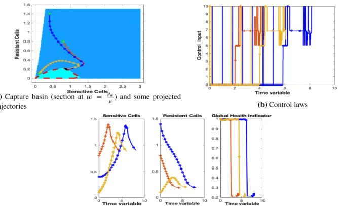
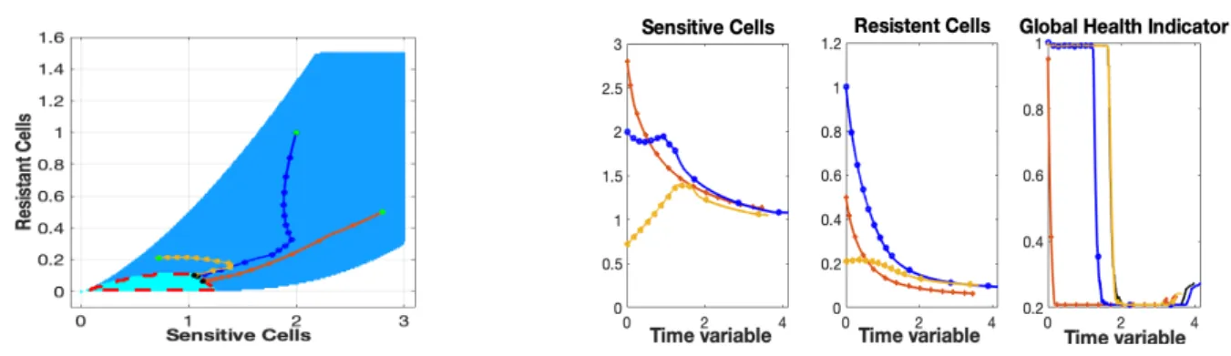
(𝑇 ) ∶= {𝑥 ∈ ℝ𝑛∣ ∃𝑢 ∈ Υ, ∀𝛼 ∈, 𝑦𝛼,𝑢[𝛼]𝑥 (𝑇 ) ∈𝕋𝑄 and 𝑦
𝛼,𝑢[𝛼]
𝑥 (𝑠) ∈ ∀𝑠 ∈ [0, 𝑇 ]}.
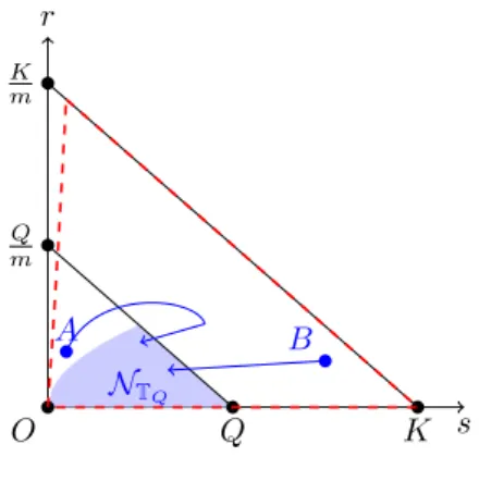
An illustration of𝕋𝑄and some trajectories reaching it are presented in Figure 1. In this figure, the filled region represents
the set𝕋𝑄. Starting from the points 𝐴 or 𝐵, it is possible to find admissible trajectories that can reach𝕋𝑄in a finite horizon
s r K m K O Q Q m A B NTQ
FIGURE 1 Illustration of the sets𝕋𝑄(filled region) and(𝑇 ) (set surrounded by the dashed line).
Notice that for some 𝑥 ∈ ℝ𝑛, it may not be possible to get to the stability kernel
𝕋𝑄 in a finite time. For example, if
𝑥= (0, 𝐾∕𝑚), then for any 𝑡≥ 0, any 𝑢 ∈ and any 𝛼 ∈ , we have 𝑦𝛼,𝑢
𝑥 (𝑡) = (0, 𝐾∕𝑚). Thus, if 𝑄 < 𝐾, whatever control is
chosen, the trajectory will never enter𝕋𝑄.
Here again, we will follow some ideas investigated by25,26,27,15and use a level-set approach to define the capture basin
(𝑇 ) at time 𝑇 .
First, we introduce the function 𝑔 ∶ ℝ𝑛 → ℝ that is the oriented distance to the set
:
𝑔𝑤(𝑥) ∶=
{
dist(𝑥, 𝜕) if 𝑥 ∈ ℝ𝑛⧵,
−dist(𝑥, 𝜕) if 𝑥 ∈ .
Now consider the control problem and its value function 𝑊 defined, for every 𝑥 ∈ ℝ𝑛and 𝑡 ∈ [0, 𝑇 ], by: 𝑊(𝑥, 𝑡) ∶= min 𝑢∈Υmax𝛼∈ { max(max 0≤𝜏≤𝑡𝑔𝑤(𝑦 𝛼,𝑢[𝛼] 𝑥 (𝜏)), 𝑉𝑄(𝑦𝛼,𝑢[𝛼]𝑥 (𝑡)) )} .
According to15, for 𝑇 > 0, the capture basin is given by:
(𝑇 ) = {𝑥 ∈ ℝ𝑛∣ 𝑊 (𝑥, 𝑇 )
≤ 0}. Moreover, the minimum time, (𝑥), for a starting position 𝑥 ∈ ℝ𝑛to reach the target
𝕋𝑄(before time 𝑇 ) is given by:
(𝑥) = min{𝑡 ∈ [0, 𝑇 ]∕𝑊 (𝑥, 𝑡) ≤ 0}. (8)
Besides, as it has been shown in15, the value function 𝑊 satisfies the following dynamical programming principle for every
𝑥∈ ℝ𝑛, for every 𝑡 ∈ [0, 𝑇 ] and ℎ ∈ [0, 𝑇 − 𝑡]: 𝑊(𝑥, 𝑡 + ℎ) = min 𝑢∈Υmax𝛼∈ ( max(max 0≤𝜏≤ℎ𝑔𝑤(𝑦 𝛼,𝑢[𝛼] 𝑥 (𝜏)), 𝑊 (𝑦 𝛼,𝑢[𝛼] 𝑥 (ℎ), 𝑡) )) ,
and 𝑊 is the unique viscosity solution to the following Hamilton-Jacobi-Bellman equation:
min(𝜕𝑡𝑊(𝑥, 𝑡) + 𝐻(𝑥, ∇𝐷𝑥(𝑥, 𝑡)), 𝑊 (𝑥, 𝑡) − 𝑔𝑤(𝑥))= 0 for 𝑥 ∈ ℝ𝑛, 𝑡∈ (0, 𝑇 ], (9a)
𝑊(𝑥, 0) = 𝑉𝑄(𝑥) for 𝑥 ∈ ℝ𝑛, (9b)
where 𝜕𝑡𝑊(𝑥, 𝑡) and 𝐷𝑥𝑊(𝑥, 𝑡) are respectively the time derivative and the space derivative (in the sense of viscosity notion,
see23).
4
TRAJECTORIES RECONSTRUCTION
Once the value functions are constructed up to some error on a grid of calculations, we want to deduce optimal controls for a starting position 𝑥0.
4.1
A trajectory staying in
𝕋𝑄Let 𝑓ℎbe a family of numerical approximations of 𝑓 . We make the following assumption:
(𝐇𝐀𝟏) for any 𝑅 > 0, there exists 𝜅𝑅>0 independant of ℎ such that: |𝑓(𝑥, 𝛼, 𝑢) − 𝑓ℎ(𝑥, 𝛼, 𝑢)| ≤ 𝜅
𝑅ℎ ∀|𝑥| < 𝑅, 𝛼 ∈ 𝐴, 𝑢 ∈ 𝑈
We will use an approximation scheme for the differential equation using 𝑓ℎ: an approximation of 𝑦𝛼,𝑢
𝑥 (𝑡) with constant 𝛼 and 𝑢will be
̃
𝑦= 𝑥 + ℎ𝑓ℎ(𝑥, 𝛼, 𝑢).
For example, the case of an Euler forward scheme corresponds to the choice 𝑓ℎ= 𝑓 .
Now, for any ℎ ∈ (0, 1) consider an approximation of 𝑉𝑄, noted 𝑉ℎ
𝑄. We make the following assumption:
(𝐇𝐀𝟐) For every ℎ ∈ (0, 1), there exists an approximation 𝑉𝑄ℎof 𝑉𝑄, which satisfies: 𝐸ℎ∶= max 𝑥 |𝑉𝑄(𝑥) − 𝑉 ℎ 𝑄(𝑥)|, 𝐸ℎ ℎ ℎ→0←→ 0.
Remark 3. The theory of approximation of viscosity solutions states that for a given time step size 𝜏, an approximation 𝑉𝑄,𝜏 of
𝑉𝑄can be computed with an error of order√𝜏. This error is guaranteed under some stability assumptions linking the time and space mesh sizes (the so-called CFL condition). So to comply with the assumption (𝐻𝐴2), one can consider the approximation
𝑉ℎ
𝑄 = 𝑉𝑄,𝜏(ℎ)where 𝜏(ℎ) = ℎ𝑘with 𝑘 > 2. In this case, 𝐸(ℎ) ℎ = 𝑂 (√ ℎ𝑘 ℎ ) = 𝑂(ℎ𝑘−22 ) ←→ ℎ→00,
and assumption (𝐻𝐴2) is satisfied.
Let ℎ ∈ (0, 1) be a time step, and 𝑁ℎ ∈ ℕ a number of steps. The actual realization of the uncertainties ̄𝛼 is known ; we will denote 𝛼𝑘= ̄𝛼(𝑘ℎ) for simplicity. For any 𝑦 ∈ ℝ2, we define the trajectory reconstruction algorithm up to time 𝑇ℎ= 𝑁ℎℎ,
described in Algorithm 1.
Algorithm 1 Stability
The starting point 𝑦 and the uncertainties realization ̄𝛼 = ( ̄𝛼𝑘)𝑘are known. Initialization Set 𝑦ℎ0 = 𝑦.
Recursive definition of 𝑦ℎ
𝑘 Suppose (𝑦 ℎ
𝓁) is known for𝓁 = 0...𝑘 − 1. To determine 𝑦 ℎ
𝑘, we define an optimal control 𝑢 ℎ 𝑘such that: 𝑢ℎ𝑘∈ argmin𝑢∈𝑈𝑉𝑄ℎ(𝑦ℎ𝑘−1+ ℎ𝑓ℎ(𝑦ℎ𝑘−1, ̄𝛼𝑘, 𝑢))𝑒−𝜆ℎ+ 𝜆ℎ𝑔𝑄(𝑦 ℎ 𝑘−1).
The new position is then defined by:
𝑦ℎ𝑘= 𝑦ℎ 𝑘−1+ ℎ𝑓 ℎ(𝑦ℎ 𝑘−1, ̄𝛼𝑘, 𝑢 ℎ 𝑘).
Complete trajectory We associate to the sequence of controls (𝑢ℎ𝑘)𝑘 the piecewise constant function 𝐮ℎ(𝑡) = 𝑢ℎ 𝑘 for 𝑡 ∈
[𝑘ℎ, (𝑘 + 1)ℎ), and an approximate trajectory 𝐲ℎdefined on [0, +∞) by:
⎧ ⎪ ⎨ ⎪ ⎩ ̇𝐲ℎ(𝑡) = 𝑓ℎ(𝑦ℎ 𝑘, ̄𝛼𝑘, 𝑢ℎ𝑘) for 𝑡 ∈ (𝑘ℎ, (𝑘 + 1)ℎ) 𝐲ℎ(𝑘ℎ) = 𝑦ℎ 𝑘 ∀𝑘 ∈ ℕ, 𝑘≤ 𝑁ℎ ̇𝐲ℎ(𝑡) = 𝑓 (𝐲(𝑡), ̄𝛼, 0) ∀𝑡 > 𝑇 ℎ
Note that in general, 𝑦𝛼,𝐮̄ ℎ
𝑦0 ≠ 𝐲
ℎ. We shall show that any accumulation point ̄𝐲 of (𝐲ℎ)
ℎis a trajectory realyzing better than a
minimum for the cost function 𝑉𝑄: since ̄𝛼 is an actual realization of the uncertainties, it might be "better than the worst".
Theorem 2. Let 𝑦 ∈ ℝ𝑛and let (𝑦ℎ
𝑘) be the sequence defined by Algorithm1, under hypothesis (𝐇𝐟) and assumptions (𝐇𝐀𝟏)
-(𝐇𝐀𝟐). Suppose furthermore the following limits to hold true:
𝑁ℎℎ ←→
ℎ→0+∞, 𝑁ℎℎ 2 ←→
Then the functions (𝐲ℎ) form a better than minimizing sequence in the following sense: 𝑉𝑄(𝑦)≥ lim sup ℎ→0 +∞ ∫ 0 𝑒−𝜆𝑡𝑔𝑄(𝐲ℎ(𝑡))𝑑𝑡 (11)
Furthermore, the family (𝐲ℎ) has an accumulation point 𝐲 in 𝑊1,1([0, +∞), 𝑒−𝑀0𝑡), and if 𝑉
𝑄(𝑦) = 0 then it is a viable trajectory,
in the sense that:
∀𝑡≥ 0, 𝐲(𝑡) ∈ 𝕋𝑄.
Proof. Let 𝑦 ∈ ℝ2and let (𝑦ℎ𝑘) and (𝑢ℎ
𝑘) be the corresponding sequences constructed by Algorithm1. One can show that there
exists 𝑅 > 0 such that for any ℎ > 0 and any 𝑛≤ 𝑁ℎ,|𝑦ℎ𝑘| ≤ 𝑅. Thus taking into account (3), there exists 𝑀𝑅such that
∀ℎ > 0, ∀𝑘≤ 𝑁ℎ,∀𝑢 ∈ 𝑈 ,|𝑓(𝑦 ℎ
𝑘, 𝛼𝑘, 𝑢)| ≤ 𝑀𝑅.
The proof of Theorem 2 is carried out in three steps.
Step 1
Let us show that there exists 𝜅 > 0 such that:
𝑉𝑄(𝑦ℎ0)≥ 𝑉𝑄(𝑦 ℎ 0+ ℎ𝑓 ℎ (𝑦ℎ0, 𝛼0, 𝑢ℎ0))𝑒−𝜆ℎ+ 𝜆ℎ𝑔𝑄(𝑦 ℎ 0) − 𝜅ℎ 2− 2𝐸 ℎ. (12)
For simplicity, we will note here 𝑦ℎ
0 = 𝑦0, and 𝑢ℎ0 = 𝑢0. Recall that the dynamical programming principle for 𝑉𝑄writes as:
𝑉𝑄(𝑦0) = min 𝑢∈Υmax𝛼∈ ⎡ ⎢ ⎢ ⎣ 𝑉𝑄(𝑦𝛼,𝑢[𝛼]𝑦 0 (ℎ))𝑒 −𝜆ℎ+ ℎ ∫ 0 𝑔𝑄(𝑦𝛼,𝑢[𝛼]𝑦 0 (𝑡))𝑒 −𝜆𝑡𝑑𝑡⎤⎥ ⎥ ⎦ . (13)
Let ̄𝑢0∈ Υ be the minimizing strategy for this problem. Let 𝛼∗be an approximation of the uncertainties, satisfying 𝛼∗(𝑡) = 𝛼 𝑘
for any 𝑡 ∈ [𝑘ℎ, (𝑘 + 1)ℎ). Then the following inequality holds:
𝑉𝑄(𝑦0)≥ 𝑉𝑄(𝑦 𝛼∗, ̄𝑢 0[𝛼∗] 𝑦0 (ℎ))𝑒 −𝜆ℎ+ ℎ ∫ 0 𝑔𝑄(𝑦𝛼∗, ̄𝑢0[𝛼∗] 𝑦0 (𝑡))𝑒 −𝜆𝑡𝑑𝑡. (14) We denote ̄𝑢0[𝛼∗] = 𝐮 𝟎∈ .
Let us consider the first term of the right-hand member of inequation (14). By convexity of 𝑓 (𝑥, 𝛼, ) for any 𝑥 ∈ ℝ𝑛and 𝛼∈ 𝐴, there exists 𝑢∗ 0∈ 𝑈 such that 𝑦0+ ℎ ∫ 0 𝑓(𝑦0, 𝛼0,𝐮𝟎(𝑡))𝑑𝑡 = 𝑦0+ ℎ𝑓 (𝑦0, 𝛼0, 𝑢∗0). Then, 𝑦𝛼∗,𝐮𝟎
𝑦0 the trajectory starting at 𝑦0for 𝑡 = 0 and following uncertainties 𝛼
∗and control 𝐮 𝟎satisfies|𝑦 𝛼∗,𝐮 𝟎 𝑦0 (ℎ) − 𝑦0| ≤ 𝑀𝑅ℎ. Moreover: |𝑦𝛼0,𝐮𝟎 𝑦0 (ℎ) − 𝑦0− ℎ𝑓 (𝑦0, 𝛼0, 𝑢∗0)| ≤ ℎ ∫ 0 |𝑓(𝑦𝛼0,𝐮𝟎 𝑦0 (𝑡), 𝛼0,𝐮𝟎(𝑡)) − 𝑓 (𝑦0, 𝛼0,𝐮𝟎(𝑡))|𝑑𝑡 ≤ ℎ ∫ 0 𝑀0|𝑦𝛼0,𝐮𝟎 𝑦0 (𝑡) − 𝑦0|𝑑𝑡 ≤ 𝑀0𝑀𝑅ℎ2,
where 𝑀0is the Lipschitz coefficient of 𝑓 . Moreover, using 𝑓ℎthe approximation of 𝑓 :
|𝑦𝛼0,𝐮𝟎
𝑦0 (ℎ) − 𝑦0− ℎ𝑓ℎ(𝑦0, 𝛼0, 𝑢0∗)| ≤ 𝑀0𝑀𝑅ℎ2+ 𝜅𝑅ℎ2.
From 2 we know that 𝑉𝑄is a Lipschitz continuous function on ℝ2; thus by denoting 𝐿𝑉 its Lipschitz coefficient:
|𝑉𝑄(𝑦 𝛼0,𝐮𝟎 𝑦0 (ℎ)) − 𝑉𝑄(𝑦0+ ℎ𝑓 ℎ (𝑦0, 𝛼0, 𝑢∗0))| ≤ 𝐿𝑉|𝑦 𝛼0,𝐮𝟎 𝑦0 (ℎ) − 𝑦0− ℎ𝑓 ℎ (𝑦0, 𝛼0, 𝑢∗0)|,
which leads to: 𝑉𝑄(𝑦𝛼0,𝐮𝟎 𝑦0 (ℎ))≥ 𝑉𝑄(𝑦0+ ℎ𝑓 ℎ(𝑦 0, 𝛼0, 𝑢∗0)) − 𝐿𝑉(𝑀0𝑀𝑅+ 𝜅𝑅)ℎ 2, ≥ 𝑉ℎ 𝑄(𝑦0+ ℎ𝑓ℎ(𝑦0, 𝛼0, 𝑢∗0)) − 𝐿𝑉((𝑀0𝑀𝑅+ 𝜅𝑅)ℎ2− 𝐸ℎ, ≥ 𝑉ℎ 𝑄(𝑦0+ ℎ𝑓ℎ(𝑦0, 𝛼0, 𝑢0)) − 𝐿𝑉((𝑀0𝑀𝑅+ 𝜅𝑅)ℎ2− 𝐸ℎ, (by definition of 𝑢0) ≥ 𝑉𝑄(𝑦0+ ℎ𝑓ℎ(𝑦0, 𝛼0, 𝐶0)) − 𝐿𝑉((𝑀0𝑀𝑅+ 𝜅𝑅)ℎ2− 2𝐸ℎ.
We now deal with the second term of (14). Since the function 𝑔𝑄is 1-Lipschitz, we get that for any 𝑡 ∈ [0, ℎ]:
|𝑔𝑄(𝑦 𝛼∗,𝐮 𝟎 𝑦0 (𝑡)) − 𝑔𝑄(𝑦0)| ≤ 𝑡 ∫ 0 |𝑓(𝑦𝛼0,𝐮𝟎 𝑦0 (𝑠), 𝛼0,𝐮𝟎(𝑠))|𝑑𝑠 ≤ 𝜅𝑅𝑡,
which leads to:
ℎ ∫ 0 𝑔𝑄(𝑦 𝛼∗,𝐮 𝟎 𝑦0 (𝑡))𝑒 −𝜆𝑡𝑑𝑡 ≥ ℎ ∫ 0 𝑔𝑄(𝑦0)𝑒−𝜆𝑡𝑑𝑡− ℎ ∫ 0 𝜅𝑅𝑡𝑒−𝜆𝑡𝑑𝑡≥ 𝜆ℎ𝑔𝑄(𝑦0) − 𝜅𝑅 ℎ2 2. Going back to (14), we get that:
𝑉𝑄(𝑦0)≥ 𝑉𝑄(𝑦0+ ℎ𝑓 ℎ
(𝑦0, 𝛼0, 𝑢0))𝑒−𝜆ℎ− 𝐿𝑉(𝐿𝑀𝑅+ 𝜅𝑅)ℎ2− 2𝐸ℎ+ 𝜆ℎ𝑔𝑄(𝑦0) − 𝐿𝑔𝜅𝑅 ℎ2
2 which concludes the demonstration of (12) by setting 𝜅 = 𝐿𝑉(𝐿𝑀𝑅+ 𝜅𝑅) + 𝐿𝑔𝜅𝑅∕2.
Step 2
We can generalize (12) to any 𝑘 < 𝑁ℎ:
𝑉𝑄(𝑦𝑘)≥ 𝑉𝑄(𝑦𝑘+ ℎ𝑓 ℎ (𝑦𝑘, 𝛼𝑘, 𝑢𝑘))𝑒−𝜆ℎ+ 𝜆ℎ𝑔𝑄(𝑦𝑘) − 2𝐸ℎ − 𝜅ℎ2. Moreover, 𝑉𝑄(𝑦0)≥ 𝑉𝑄(𝑦1)𝑒−𝜆ℎ+ 𝜆ℎ𝑔𝑄(𝑦0) − 2𝐸ℎ − 𝜅ℎ2 ≥ 𝑉𝑄(𝑦2)𝑒−2𝜆ℎ+ 𝜆ℎ(𝑔𝑄(𝑦0) + 𝑒−𝜆ℎ𝑔𝑄(𝑦1)) − 4𝐸ℎ− 2𝜅ℎ2.
By induction we deduce that:
𝑉𝑄(𝑦0)≥ 𝑉𝑄(𝑦𝑁ℎ)𝑒 −𝜆𝑁ℎℎ+ 𝜆ℎ 𝑁∑ℎ−1 𝑘=0 𝑒−𝜆𝑘ℎ𝑔𝑄(𝑦𝑘) − 2𝑁ℎ𝐸ℎ− 𝜅𝑁ℎℎ2 Step 3
Now consider the complete integral∫𝑇ℎ
0 𝑒 −𝜆𝑡𝑔 𝑄(𝐲ℎ(𝑡))𝑑𝑡. We have that: 𝑇ℎ ∫ 0 𝑒−𝜆𝑡𝑔𝑄(𝐲ℎ(𝑡))𝑑𝑡 = 𝑁∑ℎ−1 𝑘=0 (𝑘+1)ℎ ∫ 𝑘ℎ 𝑒−𝜆𝑡𝑔𝑄(𝐲ℎ(𝑡))𝑑𝑡 = 𝑁∑ℎ−1 𝑘=0 𝑒−𝑘ℎ ℎ ∫ 0 𝑒−𝜆𝑡𝑔𝑄(𝐲ℎ(𝑡 + 𝑘ℎ))𝑑𝑡 ≤ 𝑁∑ℎ−1 𝑘=0 𝑒−𝑘ℎ ℎ ∫ 0 𝑒−𝜆𝑡(𝑔𝑄(𝑦𝑘) + 𝑡𝐶𝑅)𝑑𝑡≤ 𝑁∑ℎ−1 𝑘=0 𝑒−𝑘ℎ ( 𝜆ℎ𝑔𝑄(𝑦𝑘) + ℎ2 2𝐶𝑅 ) . Moreover, +∞ ∫ 𝑇ℎ 𝑒−𝜆𝑡𝑔𝑄(𝐲ℎ(𝑡))𝑑𝑡 ≤‖𝑔𝑄‖∞𝑒−𝜆𝑇ℎ. Thus, 𝑉𝑄(𝑦0)≥ +∞ ∫ 0 𝑒−𝜆𝑡𝑔𝑄(𝐲ℎ(𝑡))𝑑𝑡 − ℎ2𝑁ℎ(𝐶𝑅 2 + 𝜅) − 2𝑁ℎ𝐸ℎ−‖𝑔𝑄‖∞𝑒 −𝜆𝑁ℎℎ. (15)
This concludes the proof of (11), since using the assumptions (10), we get; 𝑉𝑄(𝑦0)≥ lim sup ℎ→0 +∞ ∫ 0 𝑒−𝜆𝑡𝑔𝑄(𝐲ℎ(𝑡))𝑑𝑡. (16)
Finally, the functions (𝐲ℎ) are equicontinuous in 𝑊1,1([0, +∞), 𝑒−𝑀0𝑡), so they have an accumulation point 𝐲 ∈
𝑊1,1([0, +∞), 𝑒−𝑀0𝑡). Using (16), we have: 0 = 𝑉𝑄(𝑦0)≥ +∞ ∫ 0 𝑒−𝜆𝑡𝑔𝑄(𝐲(𝑡))𝑑𝑡. Therefore, the trajectory is viable, which concludes the proof of Theorem 2.
Remark 4. It is possible that, for a fixed ℎ > 0, the constructed trajectory 𝐲ℎis not viable on [0, 𝑇
ℎ]. However, because of (16),
for ℎ small enough the trajectory stays close to𝕋𝑄.
Moreover, it is possible that for an initial point 𝑦0that satisfies 𝑔𝑄(𝑦0) = 0 but 𝑉𝑄(𝑦0) > 0, for certain realizations of the
uncertainties ̄𝛼, the trajectory 𝐲 constructed by Algorithm1 is viable.
In Algorithm1, the uncertainty function ̄𝛼 is supposed to be known. This is obviously the case when the problem is without uncertainty. This algorithm is also of interest when the model is with uncertainties. It provides a tool to explore different scenarii and adjust the control depending on the variations of these uncertainties.
It is also possible to modify the algorithm to define the worst case scenario and to compute the best response to that scenario. In this case, the algorithm should be modified as shown in Algorithm 2.
Algorithm 2 Stability (worst case)
The starting point 𝑦 is known.
Initialization Set 𝑦ℎ0 = 𝑦.
Recursive definition of 𝑦ℎ
𝑘 Suppose (𝑦 ℎ
𝓁) is known for𝓁 = 0...𝑘 − 1. To determine 𝑦 ℎ
𝑘, we first define the worst value of
uncertainties: 𝛼𝑘ℎ∈ argmax𝛼∈𝐴min 𝑢∈𝑈𝑉 ℎ 𝑄(𝑦 ℎ 𝑘−1+ ℎ𝑓 ℎ (𝑦ℎ𝑘−1, 𝛼, 𝑢))𝑒−𝜆ℎ+ 𝜆ℎ𝑔𝑄(𝑦 ℎ 𝑘−1).
Then we consider the optimal control 𝑢ℎ
𝑘such that: 𝑢ℎ𝑛 ∈ argmin𝑢∈𝑈𝑉𝑄ℎ(𝑦 ℎ 𝑘−1+ ℎ𝑓 ℎ (𝑦ℎ𝑘−1, 𝛼𝑘ℎ, 𝑢))𝑒−𝜆ℎ+ 𝜆ℎ𝑔𝑄(𝑦 ℎ 𝑘−1).
The new position is then defined by:
𝑦ℎ𝑘= 𝑦ℎ𝑘−1+ ℎ𝑓ℎ(𝑦ℎ𝑘−1, 𝛼𝑘ℎ, 𝑢ℎ𝑘).
Complete trajectory We associate to the sequence of controls (𝑢ℎ
𝑘)𝑘 the piecewise constant function 𝐮ℎ(𝑡) = 𝑢ℎ𝑘 for 𝑡 ∈
[𝑘ℎ, (𝑘 + 1)ℎ), and an approximate trajectory 𝐲ℎdefined on [0, +∞) by:
⎧ ⎪ ⎨ ⎪ ⎩ ̇𝐲ℎ(𝑡) = 𝑓ℎ(𝑦ℎ 𝑘, 𝛼 ℎ 𝑘, 𝑢 ℎ 𝑘) for 𝑡 ∈ (𝑘ℎ, (𝑘 + 1)ℎ) 𝐲ℎ(𝑘ℎ) = 𝑦ℎ 𝑘 ∀𝑘 ∈ ℕ, 𝑘≤ 𝑁ℎ ̇𝐲ℎ(𝑡) = 𝑓 (𝐲(𝑡), ̄𝛼, 0) ∀𝑡 > 𝑇 ℎ
Remark 5. Algorithm 2 provides a robust trajectory with respect to any uncertainty within the range of interval 𝐴. This trajectory can be seen as a trajectory of total "victory", but it can also be seen as a pessimistic trajectory because it is foreseen in the worst case. In this perspective, the trajectories of Algorithm 1 are less pessimistic because they adjust to the value of the uncertainty if it becomes available (by measurement for example) as the trajectory evolves.
4.2
Minimal entry time
We now study how to construct optimal trajectories, knowing an approximation of 𝑊 , entering𝕋𝑄 in a minimal time. We
focus on system (M1), an extension to (M2) can be obtained with results from15.
The first algorithm we present is a direct application of the value function 𝑊 . Suppose an approximation 𝑊ℎof 𝑊 has been
constructed. Choose a starting point 𝑥0such that 𝑊ℎ(𝑥
0, 𝑇) < 0. Given a fixed perturbation ̄𝛼 ∈ , and maximal number of
time steps 𝑁 (the fixed time step being ℎ = 𝑇 ∕𝑁 ), we define the trajectory reconstruction by Algorithm3
Algorithm 3 Minimal entry time
The starting point 𝑥0and the uncertainties realization ̄𝛼 ∶= ( ̄𝛼𝑘)𝑘are known. Initialization Set 𝑦ℎ0 = 𝑥0.
Recursive definition of 𝑦ℎ
𝓁 Suppose (𝑦 ℎ
𝓁) is known for𝓁 = 0...𝑘 − 1 < 𝑁. To determine 𝑦 ℎ
𝑘, we define an optimal control 𝑢 ℎ 𝑘
such that:
𝑢ℎ𝑘∈ argmin𝑢∈𝑈𝑊ℎ(𝑦ℎ𝑘−1+ ℎ𝑓ℎ(𝑦ℎ𝑘−1, ̄𝛼𝑘, 𝑢), 𝑘ℎ) The new position is then defined by:
𝑦ℎ𝑘= 𝑦ℎ 𝑘−1+ ℎ𝑓 ℎ(𝑦ℎ 𝑘−1, 𝛼𝑘, 𝑢 ℎ 𝑘).
Complete trajectory We associate to the sequence of controls (𝑢ℎ𝑘)0≤𝑘≤𝑁−1 the piecewise constant function 𝐮ℎ(𝑡) = 𝑢ℎ 𝑘for 𝑡∈]𝑘ℎ, (𝑘 + 1)ℎ], and an approximate trajectory 𝐲ℎdefined on [0, 𝑇 ] by:
{
𝐲ℎ(𝑘ℎ) = 𝑦ℎ
𝑘 ∀𝑛 ∈ ℕ, 𝑛≤ 𝑁 ̇𝐲ℎ(𝑡) = 𝑓ℎ(𝑦ℎ
𝑘, 𝛼𝑘, 𝑢ℎ𝑘) for 𝑡 ∈ (𝑘ℎ, (𝑘 + 1)ℎ], 𝑘 < 𝑁 .
We suppose that there exists 𝐸ℎ>0 such that 𝐸ℎ∕ℎ ←→ 0 when ℎ → 0 and:
∀𝑡 > 0,||𝑊 (⋅, 𝑡) − 𝑊ℎ(⋅, 𝑡)||∞≤ 𝐸ℎ.
Then the following convergence theorem holds:
Theorem 3. Let 𝑦 ∈ ℝ2 and let (𝑦ℎ
𝑘) be the sequence defined by Algorithm 3. We suppose true the assumptions (𝐇𝐟) and
(𝐇𝐀𝟏)-(𝐇𝐀𝟐). Then the functions (𝐲ℎ) form a better than minimizing sequence in the following sense:
∀𝑡 ∈ [0, 𝑇 ], 𝑊 (𝑥, 𝑡)≤ lim sup
ℎ→0
𝑑𝑄(𝐲ℎ(𝑡))
Moreover, the family of functions 𝐲ℎadmits cluster points as ℎ → 0. Any such cluster ̄𝐲 is a trajectory of system (M1) with
uncertainties 𝛼.
This theorem can be proven by using similar arguments as in the proof of theorem (11).
Remark 6. As there might be several controls such that the trajectory is optimal, the control found by Algorithm 3 might present lots of variations depending on the implementation of the argmin function. Moreover, recall that 𝑢 represents a dosage of drug to give to a patient (or to put on a Petri dish as a first biological model). Thus, shattering controls are really not interesting for a medical application. Gratefully, as shown in Section 5, the controls found numerically are rarely shattering, so their actual implementation would be feasible.
In Algorithm 3, the the realization of the uncertainties is supposed to be known. To have a better hindsight of the adaptability of the system, we can consider the worst case scenario, were the uncertainties always take the worst value possible to delay the entrance in𝕋
𝑄. In this case, the corresponding trajectories can be obtained by Algorithm 4.
Remark 7. As mentioned in Remark 5, the worst case (Algorithm 4) provides an admissible trajectory that can reach the stability kernel for any uncertainty within the set 𝐴, whereas Algorithm 3 provides a less pessimistic trajectory that can reach a target and adjust to the values of the uncertainties if they become available.
Algorithm 4 Minimal entry time (worst case)
The starting point 𝑥0is known.
Initialization Set 𝑦ℎ
0 = 𝑥0. Recursive definition of 𝑦ℎ
𝓁 Suppose (𝑦 ℎ
𝓁) is known for𝓁 = 0...𝑘 − 1 < 𝑁. To determine 𝑦 ℎ
𝑘, we first define the worst value
of the uncertainties:
𝛼𝑘ℎ∈ argmax𝛼∈𝐴min
𝑢∈𝑈𝑊 ℎ
(𝑦ℎ𝑘−1+ ℎ𝑓ℎ(𝑦ℎ𝑘−1, ̄𝛼𝑘, 𝑢), 𝑘ℎ) We then consider the optimal control 𝑢ℎ
𝑘such that:
𝑢ℎ𝑘∈ argmin𝑢∈𝑈𝑊ℎ(𝑦ℎ𝑘−1+ ℎ𝑓ℎ(𝑦ℎ𝑘−1, ̄𝛼𝑘ℎ, 𝑢), 𝑘ℎ) The new position is then defined by:
𝑦ℎ𝑘= 𝑦ℎ𝑘−1+ ℎ𝑓ℎ(𝑦ℎ𝑘−1, 𝛼𝑘ℎ, 𝑢ℎ𝑘).
Complete trajectory We associate to the sequence of controls (𝑢ℎ
𝑘)0≤𝑘≤𝑁−1 the piecewise constant function 𝐮ℎ(𝑡) = 𝑢ℎ𝑘for 𝑡∈]𝑘ℎ, (𝑘 + 1)ℎ], and an approximate trajectory 𝐲ℎdefined on [0, 𝑇 ] by:
{ 𝐲ℎ(𝑘ℎ) = 𝑦ℎ 𝑘 ∀𝑛 ∈ ℕ, 𝑛≤ 𝑁 ̇𝐲ℎ(𝑡) = 𝑓ℎ(𝑦ℎ 𝑘, 𝛼 ℎ 𝑘, 𝑢 ℎ 𝑘) for 𝑡 ∈ (𝑘ℎ, (𝑘 + 1)ℎ], 𝑘 < 𝑁 .
5
NUMERICAL SIMULATIONS
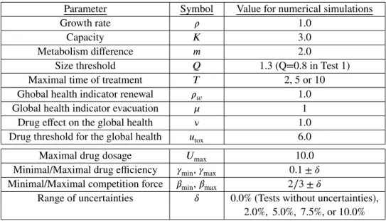
We present in this section numerical simulations solving the viability and reachability problems. The simulations were performed with the software ROC-HJ. The values of the different parameters are listed in table 1. These parameters were chosen arbitrarily to show some general numerical results.
Parameter Symbol Value for numerical simulations
Growth rate 𝜌 1.0
Capacity 𝐾 3.0
Metabolism difference 𝑚 2.0
Size threshold 𝑄 1.3 (Q=0.8 in Test 1)
Maximal time of treatment 𝑇 2, 5 or 10
Ghobal health indicator renewal 𝜌𝑤 1.0
Global health indicator evacuation 𝜇 1
Drug effect on the global health 𝜈 1.0
Drug threshold for the global health 𝑢tox 6.0
Maximal drug dosage 𝑈max 10.0
Minimal/Maximal drug efficiency 𝛾min, 𝛾max 0.1 ± 𝛿 Minimal/Maximal competition force 𝛽min, 𝛽max 2∕3 ± 𝛿
Range of uncertainties 𝛿 0.0% (Tests without uncertainties), 2.0%, 5.0%, 7.5%, or 10.0%
TABLE 1 List of parameters and their values for numerical simulations
To solve the viability and reachability problems formulated in the previous sections, we proceed by solving the corresponding Hamilton Jacobi equations. We first start with some simulations for model (M1) when there is no uncertainties in the model, in other words when the set is reduced to a singleton.
5.1
Numerical approximation of the value functions 𝑉
𝑄and 𝑊
Following Theorem 1, we know that the value function 𝑉𝑄, corresponding to the viability problem, is the unique solution of a steady HJ equation in the following form:
𝜆𝑉𝑄+ 𝐻(𝑥, ∇𝑉𝑄) − 𝑔𝑄(𝑥) = 0, 𝑥∈ ℝ𝑛,
where 𝜆 > 𝑀0 and the Hamiltonian 𝐻 is defined in Theorem 1. An approximation of 𝑉𝑄 can be obtained by a numerical discretization of this HJ equation. Note that numerical approximations of HJ equations have been studied extensively in the literature. One can cite for instance the Semi-Lagrangian methods28,29,30, or the class of finite differences methods. It is known
that a Semi-Lagrangian scheme would require a discretization of the set of the control variables. Since we have an explicit formula of 𝐻 , we prefer to use a scheme that will exploit this structure of the Hamiltonian and hence avoid the discretization of the control variables. For this reason, in all our simulations we will use a scheme based on finite difference approximations. Let Δ𝑦 = (Δ𝑦𝑘)1≤𝑘≤𝑛be a spatial discretization step (with Δ𝑦𝑘>0). Consider a uniform grid on ℝ𝑛as follows:
∶={𝑦𝑖= 𝑖Δ𝑦≡ (𝑖𝑘Δ𝑦𝑘)1≤𝑘≤𝑛, 𝑖= (𝑖1,… , 𝑖𝑛) ∈ ℤ
𝑛}. (17)
Denote {𝑒𝑘}𝑘=1,…,𝑛the canonical basis of ℝ𝑛. For a function 𝑉 ∶ → ℝ, the terms 𝐷±𝑘𝑉(𝑥) are given by: 𝐷±𝑘𝑉(𝑥) ∶= ±𝑉(𝑥 ± Δ𝑦𝑘𝑒𝑘) − 𝑉 (𝑥)
Δ𝑦𝑘
. (18)
The vectors 𝐷±𝑉(𝑥) are defined by: 𝐷±𝑉(𝑥) ∶= (𝐷±
1𝑉(𝑥),⋯ , 𝐷 ±
𝑛𝑉(𝑥)). An approximation of 𝑉𝑄can be obtained by solving
the following approximated scheme:
𝑉ℎ(𝑥) = (1 − 𝜆ℎ)𝑉ℎ(𝑥) − 𝐻Δ(𝑥, 𝐷+𝑉ℎ(𝑥), 𝐷−𝑉ℎ(𝑥)) + 𝑔(𝑥) for 𝑥 ∈
, (19)
where the numerical Hamiltonian 𝐻Δ is an approximation of the Hamiltonian function 𝐻 . The numerical approximation 𝑉ℎ∶ ℝ𝑛→ ℝ is a bilinear interpolation of {𝑉ℎ(𝑥), 𝑥 ∈}.
Following31,15, if the numerical Hamiltonian 𝐻Δ is Lipschitz continuous on all its arguments, consistent with 𝐻 (i.e., 𝐻Δ(𝑦, 𝑝, 𝑝) = 𝐻(𝑦, 𝑝)) and monotone (i.e 𝜕𝐻Δ
𝜕𝑝− 𝑘
(𝑦, 𝑝−, 𝑝+)≥ 0, 𝜕𝐻Δ
𝜕𝑝+ 𝑘
(𝑦, 𝑝−, 𝑝+) ≤ 0) together with the following
Courant-Friedrich-Levy (CFL) condition ℎ 𝑛 ∑ 𝑘=1 1 Δ𝑦𝑘 {| || | 𝜕𝐻Δ 𝜕𝑝− 𝑘 (𝑦, 𝑝−, 𝑝+)|| ||+|| ||𝜕𝐻 Δ 𝜕𝑝+𝑘 (𝑦, 𝑝 −, 𝑝+)|| || } ≤ 1,
then, as ℎ goes to 0, the numerical solution 𝑉ℎconverges uniformly, on every compact set, towards the desired solution 𝑉 𝑄.
In this paper, a simple Lax-Friedrich scheme has been used:
𝐻Δ(𝑥, 𝑝−, 𝑝+) ∶= 𝐻(𝑦,𝑝 −+ 𝑝+ 2 ) − 𝑛 ∑ 𝑘=1 𝑐𝑘 2(𝑝 + 𝑘 − 𝑝 − 𝑘), with constants 𝑐𝑘≥|𝜕𝐻
𝜕𝑝𝑘|, and a fictitious time step ℎ such that:
ℎ 𝑛 ∑ 𝑘=1 𝑐𝑘 Δ𝑦𝑘 ≤ 1. (20)
Although (19) is a nonlinear equation, the use of a fictitious time ℎ such that ℎ𝜆 < 1 guarantees that the following fixed-point algorithm converges towards a unique solution that happens to be 𝑉ℎ(see23,28,30):
•For 𝑘 = 0, consider 𝑉ℎ,0a given function on the domain of computation
•For 𝑘≥ 0, compute 𝑉ℎ,𝑘+1by:
𝑉ℎ,𝑘+1(𝑥) = (1 − 𝜆ℎ)𝑉ℎ,𝑘− 𝐻Δ(𝑥, 𝐷+𝑉ℎ,𝑘(𝑥), 𝐷−𝑉ℎ,𝑘(𝑥)) + 𝑔(𝑥) for 𝑥 ∈. (21) In practice, the above fixed-point algorithm stops at a stopping criteria:
‖𝑉ℎ,𝑘+1− 𝑉ℎ,𝑘
‖∞≤ 𝜀,
Remark 8. Instead of a fixed-point algorithm described here above, one can use a policy iterations method (or Howard algorithm), see32,33. In the rest of the paper, we prefer to focus on the analysis of the obtained results and not on the performances
of the numerical schemes. We simply use the Lax-Friederich scheme coupled with a fixed-point algorithm.
An approximation of 𝑊 is now determined through the following scheme. Let 𝑁 a given integer, denote Δ𝑡 the time dis-cretization step such that 𝑇 ∕𝑁 = 𝑑𝑡. Set 𝑡𝓁 ∶=𝓁Δ𝑡, and denote by 𝑤𝓁
𝑖 an approximation of the solution 𝑊 (𝑡𝓁, 𝑦𝑖). By using
again the Lax-Friedrich scheme, we consider the explicit scheme, as in15: 𝑤𝓁𝑖 = max ( 𝑤𝓁+1𝑖 − Δ𝑡 𝐻Δ(𝑦𝑖, 𝐷−𝑤𝓁+1𝑖 , 𝐷+𝑤𝓁+1𝑖 ), 𝑤𝓁𝑖 − 𝑔𝑤(𝑦𝑖) ) , (22a) 𝓁 ∈ {1 ⋯ , 𝑁} 𝑦𝑖 ∈ 𝑤0𝑖 = 𝑉𝑄(𝑦𝑖) for 𝑦𝑖∈, (22b)
and we denote 𝑊Δthe interpolation of (𝑊𝓁
𝑖 )𝑙,𝑖on (𝑡𝑙, 𝑥𝑖)𝓁,𝑖. Remark 9. Under the CFL condition:
Δ𝑡 𝑛 ∑ 𝑘=1 𝑐𝑘 Δ𝑦𝑘 ≤ 1,
the scheme (22) produces a numerical approximation 𝑊Δthat converges to the desired solution 𝑊 , as Δ = (Δ𝑡, Δ𝑦) go to 0
(see15for more details).
Notice that Algorithm 2 of trajectory reconstrunction requires the values of the approximate function 𝑊Δat every time step 𝑡𝓁. It means, that the values 𝑤𝓁⋅ should be stored on the grid at each time step. To reduce the storage effort, we can use the
minimaltime function mapping defined in (8). Indeed, while computing the approximation 𝑊Δ, we can obtain and store an
approximationΔas follows:
For𝓁 = 0, setΔ,0(𝑦
𝑖) = 0 if 𝑉𝑄(𝑦𝑖)≤ 0, and Δ,0(𝑦𝑖) = +∞ otherwise;
For𝓁≥ 1, once 𝑤𝓁
𝑖 is computed, the minimum time function can be updated by:
Δ,𝓁(𝑦 𝑖) = { 𝑡𝓁 if 𝑤𝓁 𝑖 ≤ 0 and Δ,𝓁−1(𝑦 𝑖) = +∞, Δ,𝓁−1(𝑦 𝑖) otherwise.
An algorithm of reconstruction, based on the minimum time functionΔ can be considered (insted of Algorithm 3). We
describe it in Algorithm 5
Algorithm 5 Minimal entry time, usingΔ
Let 𝑥0∈ be the starting point and consider the given uncertainty realization ̄𝛼.
Initialization Set 𝑦ℎ0 = 𝑥0.
Recursive definition of 𝑦ℎ
𝓁 Suppose (𝑦 ℎ
𝓁) is known for𝓁 = 0...𝑘 − 1 < 𝑁. To determine 𝑦 ℎ
𝑘, we define an optimal control 𝑢 ℎ 𝑘
such that:
𝑢ℎ𝑘∈ argmin𝑢∈𝑈ℎ
(𝑦ℎ𝑘−1+ ℎ𝑓ℎ(𝑦ℎ𝑘−1, ̄𝛼𝑘, 𝑢)) The new position is then defined by:
𝑦ℎ𝑘= 𝑦ℎ 𝑘−1+ ℎ𝑓
ℎ(𝑦ℎ
𝑘−1, ̄𝛼𝑘, 𝑢ℎ𝑘).
Complete trajectory We associate to the sequence of controls (𝑢ℎ𝑘)0≤𝑘≤𝑁−1 the piecewise constant function 𝐮ℎ(𝑡) = 𝑢ℎ 𝑘for 𝑡∈]𝑘ℎ, (𝑘 + 1)ℎ], and an approximate trajectory 𝐲ℎdefined on [0, 𝑇 ] by:
{
𝐲ℎ(𝑘ℎ) = 𝑦ℎ
𝑘 ∀𝑘 ∈ ℕ, 𝑘≤ 𝑁 ̇𝐲ℎ(𝑡) = 𝑓ℎ(𝑦ℎ