HAL Id: hal-01649244
https://hal.inria.fr/hal-01649244v2
Submitted on 5 Dec 2017
HAL is a multi-disciplinary open access
archive for the deposit and dissemination of
sci-entific research documents, whether they are
pub-lished or not. The documents may come from
teaching and research institutions in France or
L’archive ouverte pluridisciplinaire HAL, est
destinée au dépôt et à la diffusion de documents
scientifiques de niveau recherche, publiés ou non,
émanant des établissements d’enseignement et de
recherche français ou étrangers, des laboratoires
Sparse Direct Solvers
Patrick Amestoy, Jean-Yves l’Excellent, Gilles Moreau
To cite this version:
Patrick Amestoy, Jean-Yves l’Excellent, Gilles Moreau. On Exploiting Sparsity of Multiple
RightHand Sides in Sparse Direct Solvers. [Research Report] RR9122, ENS de Lyon; INRIA Grenoble
-Rhone-Alpes. 2017, pp.1-28. �hal-01649244v2�
0249-6399 ISRN INRIA/RR--9122--FR+ENG
RESEARCH
REPORT
N° 9122
Décembre 2017On Exploiting Sparsity of
Multiple Right-Hand
Sides in Sparse Direct
Solvers
RESEARCH CENTRE GRENOBLE – RHÔNE-ALPES
Inovallée
655 avenue de l’Europe Montbonnot
Right-Hand Sides in Sparse Direct Solvers
Patrick Amestoy
∗, Jean-Yves L’Excellent
†, Gilles Moreau
† Project-Team ROMAResearch Report n° 9122 — Décembre 2017 — 28 pages
Abstract: The cost of the solution phase in sparse direct methods is sometimes critical. It
can be larger than the one of the factorization in applications where systems of linear equations with thousands of right-hand sides (RHS) must be solved. In this paper, we focus on the case of multiple sparse RHS with different nonzero structures in each column. Given a factorization A = LU of a sparse matrix A and the system AX = B (or LY = B when focusing on the forward elimination), the sparsity of B can be exploited in two ways. First, vertical sparsity is exploited by pruning unnecessary nodes from the elimination tree, which represents the dependencies between computations in a direct method. Second, we explain how horizontal sparsity can be exploited by working on a subset of RHS columns at each node of the tree. A combinatorial problem must then be solved in order to permute the columns of B and minimize the number of operations. We propose a new algorithm to build such a permutation, based on the tree and on the sparsity structure of B. We then propose an original approach to split the columns of B into a minimal number of blocks (to preserve flexibility in the implementation or maintain high arithmetic intensity, for example), while reducing the number of operations down to a given threshold. Both algorithms are motivated by geometric intuitions and designed using an algebraic approach, and they can be applied to general systems of linear equations. We demonstrate the effectiveness of our algorithms on systems coming from real applications and compare them to other standard approaches. Finally, we give some perspectives and possible applications for this work.
Key-words: sparse linear algebra, sparse matrices, direct method, multiple sparse right-hand
sides
∗University of Toulouse, INPT and IRIT laboratory, France †University of Lyon, Inria and LIP laboratory, France
solveurs creux directs
Résumé : Le coût des résolutions triangulaires des solveurs creux directs est parfois critique.
Ce coût peut dépasser celui de la factorisation dans les applications qui nécessitent la résolution de plusieurs milliers de seconds membres. Cette étude se concentre sur les cas où les seconds membres sont multiples, creux et n’ont pas tous la même structure.
Étant donnée la factorisation A = LU d’une matrice creuse A, l’étude met surtout l’accent sur la résolution du premier système triangulaire LY = B, où L est triangulaire inférieure. Dans ce type de problèmes, le creux dans la matrice B peut être exploité de deux manières. Premièrement, on évite le calcul de certaines lignes, ce qui correspond à élaguer certains nœuds de l’arbre d’élimination (qui représente les dépendances entre les calculs de la résolution). Deuxièmement, on réduit, pour chaque nœud, le calcul sur des sous-ensembles de colonnes de B plutôt que sur la matrice complète. Dans ce cas, un problème combinatoire doit être résolu afin de trouver une permutation des colonnes de B.
S’appuyant d’abord sur l’algorithme de dissection emboitée appliqué à un domaine régulier, un premier algorithme est proposé pour contruire une permutation des colonnes de B. Puis une nouvelle approche permet de poursuivre la réduction du nombre d’opérations grâce à la création de blocs. Pour préserver la flexibilité de l’implémentation ainsi que l’efficacité des opérations de type BLAS 3, un nombre minimal de groupe est créé. Inspirés d’abord par des observations géométriques, ces nou-veaux algorithmes ont été étendus algébriquement pour n’utiliser que des informations provenant de la structure des seconds membres et des arbres d’élimination. Ils permettent ainsi une conver-gence rapide vers le nombre minimal d’opérations. Les résultats expérimentaux démontrent le gain obtenu par rapport à d’autres approches classiques. Enfin, les applications et extensions possibles de ce travail sont présentées.
Mots-clés : Algèbre linéaire creuse, matrices creuses, méthode directe, seconds membres creux
Introduction
We consider the direct solution of sparse systems of linear equations
AX = B, (1)
where A is an n × n sparse matrix with a symmetric structure and B is an n × m matrix of right-hand sides (RHS). When A is decomposed under the form A = LU with a sparse direct method [7],
e.g., the multifrontal method [8], the solution can be obtained by forward and backward triangular
solves involving L and U . In this study, we are interested in the situation where not only A is sparse, but also B, with the columns of B possibly having different structures, and we focus on the efficient solution of the forward system
LY = B, (2)
where the unknown Y and the right-hand side B are n × m matrices. We will see in this study that the ideas developed for Equation (2) are indeed more general and can be applied in a broader context. In particular, they can be applied to the backward substitution phase, in situations where the system U X = Y must be solved for a subset of the entries in X [3,17,19,20]. In direct methods, the dependencies of the computations for factorization and solve operations can be represented by a tree [13], which plays a central role and expresses parallelism between tasks. The factorization phase is usually the most costly phase but, depending on the number of columns m in B or on the number of systems to solve with identical A and different B, the cost of the solve phase may also be significant. As an example, electromagnetism, geophysics or imaging applications can lead to systems with sparse multiple right-hand sides for which the solution phase is significantly more costly than the factorization phase [1,16]. Such applications motivate the algorithms presented in this study.
A sparse RHS is characterized by its set of nonzeros and it is worth considering a RHS as sparse when doing so improves performance or storage compared to the dense case. The exploitation of RHS sparsity (later extended to reduce computations when only a subset of the solution is needed [17, 19]) was formalised by Gilbert [10] and Gilbert and Liu [11], who showed that the structure of the solution Y from Equation (2) can be predicted from the structures of L and B. From this structure prediction, one can design mechanisms to reduce computation. In particular, tree pruning suppresses nodes in the elimination tree involving only computations on zeros. When solving a problem with multiple RHS, the preferred technique is usually to process all the RHS in one shot. The subset of the elimination tree to be traversed is then the union of the different pruned trees (see Section 2.1). However, when the RHS have different structures, this means that extra operations on zeros have to be performed. In order to limit these extra operations, several approaches may be applied. The one that minimizes the number of operations consists in processing the RHS columns one by one, each time with a different pruned tree. However, such an approach is not practical and leads to a poor arithmetic intensity (e.g., it will not exploit level 3 BLAS [6]). Another approach, in the context of blocks of RHS with a predetermined number of columns in each block, consists in applying heuristics to determine which columns to include within which block. The objective function to minimize might be the volume of accesses to the factor matrices [3], or the number of operations [18]. When possible, large sets of columns, possibly the whole set of m columns, may be processed in one shot. Thanks to the different sparsity structure of each column of B, it is then possible to work on less than m columns at most nodes in the tree, as explained in Section 2.2. Such a mechanism has been introduced in the context of the parallel computation of
entries of the inverse [4], where at each node, computations are performed on a contiguous interval of RHS columns.
After a description of these mechanisms with illustrative examples, one contribution of this work is to propose algorithms that improve the exploitation of column intervals at each node. A geometrical intuition motivates a new approach to obtain a permutation of the columns of B that significantly reduces computation during (2) with respect to previous work. The algorithm is first introduced for a nested dissection ordering and for a regular mesh, then generalized to arbitrary elimination trees. Computation can then be further reduced by dividing the RHS into blocks. However, instead of enforcing a constant number of columns per block, our objective is to minimize the number of blocks created. If ∆min(B) represents the number of operations to solve (2) when
processing the RHS columns one by one, we show on real applications that our blocking algorithm can approach ∆min(B) within a tolerance of 1% while creating a small number of blocks. Please
note that RHS sparsity limits the amount of tree parallelism because only a few branches are traversed in the elimination tree. Therefore, whenever possible, our heuristics also aim at choosing the approach that maximizes tree parallelism.
This paper is organized as follows. Section 1 presents the general context of our study and Section 2 exposes the classical tree pruning technique together with the notion of node intervals where different intervals of columns may be processed at each node of the tree. In Section 3, we introduce a new permutation to reduce the size of such intervals and thus limit the number of operations, first using geometrical considerations for a regular nested dissection ordering, then with a pure algebraic approach that can then be applied in a general case and for arbitrary right-hand sides. We call it the Flat Tree algorithm because of the analogy with the ordering that one would obtain when “flattening” the tree. In Section 4, an original blocking algorithm is then introduced to further improve the flat tree ordering. It aims at defining a limited number of blocks of right-hand sides to minimize the number of operations while preserving parallelism. Section 5 gives experimental results on a set of systems coming from two geophysics applications relying on Helmholtz or Maxwell equations. Section 6 discusses adaptations of the nested dissection algorithm to further decrease computation and Section 7 shows why this work has a broader scope than solving Equation (2) and presents possible applications.
1
Nested dissection, sparse direct solvers and triangular solve
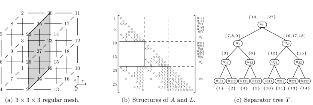
In sparse direct methods, the order of the variables of a sparse matrix A strongly impacts the number of operations for the factorization, the size of the factor matrices, and the cost of the solve phase. We illustrate in Figure 1 the use of nested dissection on a regular mesh [9].
The nested dissection algorithm consists in dividing domains with separators. The regular 3×3×3 domain shown in Figure 1(a) is first divided by a 3×3 constant-x plane separator (variables {19, . . . , 27} forming separator u0) into two even subdomains. Each subdomain is then divided
recursively (constant-y plane separators {16, 17, 18} and {7, 8, 9}, etc.). By ordering the separators after the subdomains, large blocks of zeros limit the amount of computation (Figure 1(b)). Although it could be different, the order inside each separator is similar to [9, Appendix].
The elimination tree [13] represents dependencies between computations: it is processed from bottom to top in the factorization and forward elimination, and from top to bottom in the backward substitution. The elimination tree may be compressed thanks to the use of supernodes, leading to a tree identical to the separator tree of Figure 1(c) when choosing supernodes identical to the
sepa-x z y 1 4 2 5 10 11 13 14 3 6 12 15 7 9 8 16 18 17 19 20 21 22 23 24 25 26 27
(a) 3 × 3 × 3 regular mesh.
1 5 10 15 20 25 × × × × × × × × × × × × × × × × × × × × × × × × × × × × × × × × × × × × × × × × × × × × ×× × × × × × × × × × × × × ×× × × × ×× × × × × × ×× ×× ××× ×××× f f f f f f f f f f f f f f f f f f f fff f f f f f f f f f f f f f f f f f f f f f f f f f f f f f f f f f f f f f f f f f f f f f f f f f f f f f f f f f f f f f f u0 u2 u21 u211 u212 u22 u221 u222 u1 u11 u111 u112 u12 u121 u122 (b) Structures of A and L. u0 u2 u22 u222 u221 u21 u212 u211 u1 u12 u122 u121 u11 u112 u111 {19, . . . ,27} {16,17,18} {15} {14} {13} {12} {11} {10} {7,8,9} {6} {5} {4} {3} {2} {1} (c) Separator tree T .
Figure 1: (a) A 3D mesh with a 7-point stencil. Mesh nodes are numbered according to a nested dissection ordering. (b) Corresponding matrix with initial nonzeros (×) in the lower triangular part of a symmetric matrix A and fill-in (f ) in the L factor. (c) Separator tree, also showing the sets of variables to be eliminated at each node.
rators resulting from the nested dissection algorithm1. We note that the order in which tree nodes
are processed (u111, u112, u11, . . . , u0), represented on the right of the matrix, is a postordering:
nodes in any subtree are processed consecutively.
L11 U11 L21 U12 βu αu
Figure 2: Structure of the factors associated to a node u of the tree.
Considering a single RHS b and the decomposition A = LU , the solution of the triangular system Ly = b (and U x = y) relies on block operations at each node of the tree T . Figure 2 represents the L and U factors restricted to a given node u of T , where the diagonal block is formed of the two lower and upper triangular matrices L11 and U11, and the update matrices are L21 and U12. The αu variables are the ones of node (or separator) u, and the βu variables correspond to the nonzero
rows in the off-diagonal parts of the L factor restricted to node u (Figure 1(b)), that have been gathered together. For example, node u1 from Figure 1 corresponds to separator {7, 8, 9}, so that L11and U11are of order αu1 = 3 and there are βu1 = 9 update variables {19, . . . , 27}, so that L21is
of size 9 × 3 (and U12 is of size 3 × 9). Starting with y ← b, the active components of y are gathered
into two temporary dense vectors y1 of size αu and y2 of size βu at each node u of T , where the
triangular solve
y1← L−111y1, (3)
1Note that in this example, identifying supernodes to separators leads to relaxed supernodes: although some
sparsity exists in the interaction of u7 and u0 (and u112 and u0), the interaction is considered dense and few
is performed, followed by the update operation
y2← y2− L21y1. (4)
y1 and y2 can then be scattered back into y, and y2 will be used at higher levels of T . When the
root is processed, y contains the solution of Ly = b. Because the matrix blocks in Figure 2 are considered dense, there are αu(αu− 1) arithmetic operations for the triangular solution (3) and
2αuβu operations for the update operation (4), leading to a total number of operations
∆ = X
u∈T
δu, (5)
where δu= αu× (αu− 1 + 2βu) is the number of arithmetic operations at node u.
2
Exploitation of sparsity in right-hand sides
In this section, we review two approaches to exploit sparsity in B when solving the triangular system (2). The first one, called tree pruning [11, 17] and explained in Section 2.1, consists in pruning the nodes at which only computations on zeros are performed. The second one, presented in Section 2.2, goes further by working on different sets of RHS columns at each node of the tree [4].
2.1
Tree pruning
Consider a non-singular n × n matrix A with a nonzero diagonal, and its directed graph G(A), with an edge from vertex i to vertex j if aij 6= 0. Given a vector b, let us define struct(b) =
{i, bi 6= 0} as its nonzero structure, and closureA(b) as the smallest subset of vertices of G(A)
including struct(b) without incoming edges. Gilbert [10, Theorem 5.1] characterizes the structure of the solution of Ax = b by the relation struct(A−1b) ⊆ closureA(b), with equality in case there
is no numerical cancellation. In our context of triangular systems, ignoring such cancellation, struct(L−1b) = closureL(b) is also the set of vertices reachable from struct(b) in G(LT), where
edges have been reversed [11, Theorem 2.1]. Finding these reachable vertices can be done using the transitive reduction of G(LT), which is a tree (the elimination tree) when L results from the factorization of a matrix with symmetric (or symmetrized) structure.
Since we work with a tree T with possibly more than one variable to eliminate at each node, let us define Vb as the set of nodes in T including at least one element of struct(b). The structure
of L−1b can be obtained by following paths from the nodes of Vb upto the root and these will be
the only nodes needed to compute L−1b. The tree consisting of this subset of nodes is what we call the pruned tree for b, and we note it Tp(b). Thanks to this pruned tree, the number of operations
∆ from Equation (5) now depends on b:
∆(b) = X
u∈Tp(b)
δu. (6)
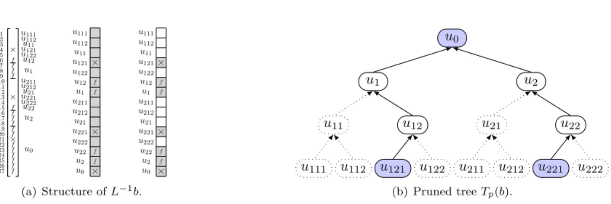
Example 2.1. Let b be a vector with nonzeros at positions 4, 13, and 21. The corresponding tree nodes are given by Vb= {u121, u221, u0}, see Figures 1 and 3. Following the paths in T from nodes
in Vb to the root results in the pruned tree of Figure 3(b). Compared to ∆ = 288 in the case of a
1 2 3 4 5 6 7 8 9 10 11 12 13 14 15 16 17 18 19 20 21 22 23 24 25 26 27 × × × f f f f f f f f f f f f f f f f u0 u2 u21 u211 u212 u22 u221 u222 u1 u11 u111 u112 u12 u121 u122 × f f × f f × u0 u2 u22 u222 u221 u21 u212 u211 u1 u12 u122 u121 u11 u112 u111 × f f × f f × u0 u2 u22 u222 u221 u21 u212 u211 u1 u12 u122 u121 u11 u112 u111 (a) Structure of L−1b. u0 u2 u22 u222 u221 u21 u212 u211 u1 u12 u122 u121 u11 u112 u111 (b) Pruned tree Tp(b).
Figure 3: Illustration of Example 2.1. (a) Structure of L−1b with respect to matrix variables (left) and to tree nodes (middle and right). × corresponds to original nonzeros and f to fill-in. In the dense case (middle) and the sparse case (right), gray parts of L−1b are the ones involving computation. (b) Pruned tree Tp(b): pruned nodes and edges are represented with dotted lines and
nodes in Vb are filled.
We now consider the case of multiple RHS (Equation (2)), where RHS columns may have different structures and denote by Bi the columns of B, for 1 ≤ i ≤ m. Instead of solving m linear
systems with each pruned tree Tp(Bi), one generally prefers to favor matrix-matrix computations
for performance reasons. For that, a first approach consists in considering VB =S1≤i≤mVBi, the
union of all nodes in T with at least one nonzero from matrix B, and the pruned tree Tp(B) =
S
1≤i≤mTp(Bi) containing all nodes in T reachable from nodes in VB. In that case, triangular and
update operations (3) and (4) become Y1← L−111Y1 and Y2← Y2− L21Y1, at each node of the tree.
The number of operations can then be defined as:
∆(B) = m × X
u∈Tp(B)
δu. (7)
Example 2.2. Figure 4(a) shows a RHS matrix B = [{B11,1}, {B6,2}, {B13,3},{B10,4}, {B2,5}] in
terms of original variables (1 to 27) and in terms of tree nodes (VB = {u212, u12, u221, u211, u112}).
In Figure 4(a), × corresponds to an initial nonzero in B and f corresponds to “fill-in” that appears
in L−1B during the forward elimination on the nodes that are on the paths from nodes in VBto the
root (see Figure 4(b)). We have ∆(B) = 5 × 264 = 1320 and ∆(B1) + ∆(B2) + . . . + ∆(B5) = 744.
At this point, we exploit tree pruning but perform extra operations by considering globally Tp(B) instead of each individual pruned tree Tp(Bi). In other words, we only exploit the vertical
sparsity of B. Processing B by smaller blocks of columns would further reduce the number of operations at the cost of more traversals of the tree and a smaller arithmetic intensity, with a minimal number of operations ∆min(B) =Pi=1,m∆(Bi) reached when B is processed column by
column, as in Figure 4(a)(right). We note that performing this minimal number of operations while traversing the tree only once (and thus accessing the L factor only once) from leaves to root would require performing complex and costly data manipulations at each node u with copies and indirect accesses to work only on the active columns of B at u. We present in the next section a simpler approach which consists in exploiting the notion of intervals of columns at each node u ∈ Tp(B).
1 2 3 4 5 6 7 8 9 10 11 12 13 14 15 16 17 18 19 20 21 22 23 24 25 26 27 × × × × × f f f f f f f f f f f f f f f f f f f f f f f f f f f f f f f f f f f f f f f f f f f f f f f f f f f f f f f f f f f f f f f f u0 u2 u21 u211 u212 u22 u221 u222 u1 u11 u111 u112 u12 u121 u122 × f f f × f f × f f f × f f f × f f f u0 u2 u22 u222 u221 u21 u212 u211 u1 u12 u122 u121 u11 u112 u111 1 2 3 4 5 1 × f f f 2 × f f 3 × f f f 4 × f f f 5 × f f f (a) Structures of L−1B, L−1B1, . . . , L−1B5. u0 u2 u22 u222 u221 u21 u212 u211 u1 u12 u122 u121 u11 u112 u111 (b) Pruned tree Tp(B) = Tp(B1) ∪ . . . ∪ Tp(B5). Figure 4: Illustration of multiple RHS and tree pruning corresponding to Example 2.2. Gray parts of L−1B (resp. of L−1Bi) are the ones involving computations when RHS are processed in one shot
(resp. one by one).
2.2
Working with column intervals at each node
Given a matrix B, we associate to a node u ∈ Tp(B) its set of active columns
Zu= {j ∈ {1, . . . , m} | u ∈ Tp(Bj)} . (8)
The intervalJmin(Zu), max(Zu)K includes all active columns, and its length is θ(Zu) = max(Zu) − min(Zu) + 1.
Zu is sometimes defined for an ordered or partially ordered subset R of the columns of B, in
which case we use the notations Zu|R, and θ(Zu|R). For u in Tp(B), Zu is non-empty and θ(Zu)
is different from 0. The main idea is then to perform the operations (3) and (4) on the θ(Zu)
contiguous columnsJmin(Zu), max(Zu)K instead of the m columns of B , leading to
∆(B) = X
u∈Tp(B)
δu× θ(Zu). (9)
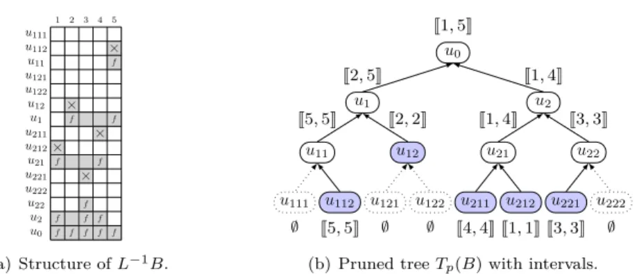
Example 2.3. In Example 2.2, there are nonzeros in columns 1 and 4 at node u21so that Zu21 =
{1, 4} (see Figure 5). Instead of performing the solve operations on all 5 columns at node u21, we
limit the computations to the θ(Zu21) = 4 columns of interval J1, 4K (and to a single column at,
e.g., node u221). Overall, ∆(B) is reduced from 1320 to 948 (while ∆min(B) = 744).
It is clear from Example 2.3 that θ(Zu) and ∆(B) strongly depend on the order of the columns
in B. In Section 3, we formalize the problem of permuting the columns of B and propose a new heuristic to find such a permutation. In Section 4, we further decrease the number of operations by identifying and extracting “problematic” columns.
3
Permuting RHS columns
We showed in Section 2.2 that horizontal sparsity can be exploited thanks to column intervals. The number of operations to solve (2) then depends on the permutation of the columns of B and we
× f f f × f f × f f f × f f f × f f f u0 u2 u22 u222 u221 u21 u212 u211 u1 u12 u122 u121 u11 u112 u111 1 2 3 4 5 (a) Structure of L−1B. u0 u2 u22 u222 u221 u21 u212 u211 u1 u12 u122 u121 u11 u112 u111 J1, 5K J1, 4K J3, 3K ∅ J3, 3K J1, 4K J1, 1K J4, 4K J2, 5K J2, 2K ∅ ∅ J5, 5K J5, 5K ∅
(b) Pruned tree Tp(B) with intervals.
Figure 5: Column intervals corresponding to Example 2.3: in gray (a) and above/below each node (b).
express the corresponding minimization problem as:
Find a permutation σ of {1, . . . , m} that minimizes ∆(B, σ) =P
u∈ Tp(B)δu× θ(σ(Zu)),
where σ(Zu) = {σ(i) | i ∈ Zu} , and
θ(σ(Zu)) is the length of the permuted intervalJmin(σ(Zu)), max(σ(Zu))K.
(10)
Rather than trying to solve the global problem with linear optimization techniques, we will propose a cheap heuristic based on the tree structure. We first define the notion of node optimality.
Definition 3.1. Given a node u in Tp(B), and a permutation σ of {1, . . . , m}, we say that we have
node optimality at u, or that σ is u−optimal if and only if θ(σ(Zu)) = #Zu, where #Zu is the
cardinal of Zu. Said differently, σ(Zu) is a set of contiguous elements.
Remark that θ(σ(Zu)) − #Zuis the number of extra columns (or padded zeros) on which extra
computation is performed and is equal to 0 in case σ is u−optimal.
Example 3.1. Consider the RHS structure of Figure 5(a) and the identity permutation. We have node optimality at u0 because #Zu0 = #{1, 2, 3, 4, 5} = 5 = θ(Zu0). We do not have
node optimality at u1 and u2 because the numbers of padded zeros are θ(Zu1) − #Zu1 = 2 and
θ(Zu2)−#Zu2 = 1, respectively. Our aim is thus to find a permutation σ that reduces the difference
θ(σ(Zu)) − #Zu.
In the following, we first present a permutation based on a postordering of Tp(B), then expose
our new heuristic, which targets node optimality in priority at the nodes near the top of the tree.
3.1
The Postorder permutation
In Figure 1, the sequence [u111, u112, u11, u121, u122, u12, u1, u211, u212, u21, u221, u222, u22, u2, u0] used to order the matrix follows a postordering: any subtree contains a set of consecutive nodes
in that sequence. This postordering is also the basis to permute the columns of B:
Definition 3.2. Consider a postordering of the tree nodes u ∈ T , and a RHS matrix B = [Bj]j=1...m
said to be postordered if and only if: ∀j1, j2, 1 ≤ j1< j2 ≤ m, we have either u(Bj1) = u(Bj2), or
u(Bj1) appears before u(Bj2) in the postordering. In other words, the order of the columns Bj is
compatible with the order of their representative nodes u(Bj).
The postordering has been applied [3,17,18] to group together in regular chunks RHS columns with “nearby” pruned trees, thereby limiting the accesses to the factors or the amount of compu-tation. It was also experimented together with node intervals [4] to RHS with a single nonzero per column, although it was then combined with an interleaving mechanism for parallel issues.
Remark that the RHS B of Figure 5(a) only has one initial nonzero per column. The represen-tative nodes for each column are u212, u12, u221, u211, and u112, respectively. The initial natural
order of the columns (INI) induces computation on explicit zeros represented by gray empty cells and we had ∆(B) = ∆(B, σINI) = 948 and ∆min(B) = 744 (see Example 2.3). On the other hand,
the postorder permutation, σPO, reorders the columns of B so that the order of their representative
nodes u112, u12, u211, u212, u221is compatible with the postordering and avoids computations on
ex-plicit zeros. In this case, there are no gray empty cells (see Figure 6(a)) and ∆(B, σPO) = ∆min(B).
More generally, it can be shown that the postordering induces no extra computations for RHS with a single nonzero per column [4].
For applications with multiple nonzeros per RHS, each column Bj may correspond to a set VBj
with more than one node, among which a representative node should be chosen. We describe two strategies. The first one, called PO_1, chooses as representative node the one corresponding to the first nonzero found in Bj (in the natural order associated to the physical problem). The second
one, called PO_2, chooses as representative node in VBj the one that appears first in the sequence of
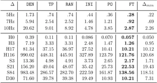
postordered nodes of the tree. A comparison of the two postorders with the initial natural order is provided in Table 1, for four problems presented in Table 2 of Section 5. Note that the initial order depends on the physical context of the application and has some geometrical properties. Table 1
Table 1: Comparison of the number of operations (×1013) between postorder strategies PO_1 and
PO_2.
∆ INI PO_1 PO_2 ∆min
H0 .086 .076 .070 .050 H3 2.48 1.69 1.47 .95 5Hz .44 .44 .36 .22 7Hz 1.46 1.48 1.21 .69
shows that the choice of the representative node has a significant impact. The superiority of PO_2 over PO_1 is clear and is larger when the number of nonzeros per RHS column is large (problems 5Hz and 7Hz). Indeed, PO_1 is even worse than the initial order on problem 7Hz.
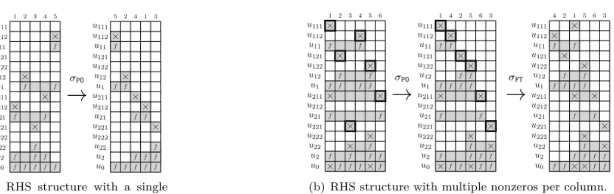
Example 3.2. Let B = [B1, B2, B3, B4, B5, B6] = [{B1,1, B10,1, B19,1}, {B4,2}, {B13,3, B15,3},{B2,3},
{B5,4, B14,4, B22,4}, {B10,5}] be the RHS represented in Figure 6(b). In terms of tree nodes, we
have: VB1 = {u111, u211, u0}, VB2 = {u121}, etc. Because the rows of B have already been
permuted according to the postordering of the tree, the representative nodes for strategies PO_1 and PO_2 are in both cases the nodes u111, u121, u221, u112, u122, u211 (cells with a bold
con-tour), for columns B1, B2, B3, B4, B5, B6, respectively. The postorder permutation yields σPO(B) =
[B1, B4, B2, B5, B6, B3], which reduces the number of gray cells and the volume of computation with
respect to the original column ordering: ∆(B) = 1368 becomes ∆(B, σPO) = 1242. Computations on padded zeros still occur, for example at nodes u211and u21where θ(σPO(Zu211)) = θ(σPO(Zu21)) = 5
× f f f × f f × f f f × f f f × f f f u0 u2 u22 u222 u221 u21 u212 u211 u1 u12 u122 u121 u11 u112 u111 1 2 3 4 5
→
σPO × f f f × f f × f f f × f f f × f f f u0 u2 u22 u222 u221 u21 u212 u211 u1 u12 u122 u121 u11 u112 u111 5 2 4 1 3(a) RHS structure with a single nonzero per column.
× f f × f f × × f f f × × f f × f f f × f f × f f × × f f f u0 u2 u22 u222 u221 u21 u212 u211 u1 u12 u122 u121 u11 u112 u111 1 2 3 4 5 6
→
σPO × f f × f f × × f f f × × f f × f f f × f f × f f × × f f f u0 u2 u22 u222 u221 u21 u212 u211 u1 u12 u122 u121 u11 u112 u111 1 4 2 5 6 3→
σFT × f f f × f f f × f f × f f × × f f × f f × × f f f × × f f u0 u2 u22 u222 u221 u21 u212 u211 u1 u12 u122 u121 u11 u112 u111 4 2 1 5 6 3(b) RHS structure with multiple nonzeros per column.
Figure 6: Illustration of the permutation σPObased on a postordering strategy on two RHS with (a)
a single initial nonzero per column (Example 2.2), and (b) multiple nonzeros per column (Example 3.2).
whereas #Zu211= #Zu21 = 2. In Figure 6(b), we represented another permutation σFTthat will be
discussed in the next section and that yields ∆(B, σFT) = 1140.
Remark that the quality of σPO depends on the original postordering. In Example 3.2, if u111
and u112 were exchanged in the original tree postordering, B1 and B4 would be swapped, and ∆
would be further improved. A possible drawback of the postorder permutation is also that, since the position of a column is based a single representative node, some information on the RHS structure is unused. We now present a more general and powerful heuristic.
3.2
The Flat Tree permutation
With the aim of satisfying node optimality (see Definition 3.1), we present another algorithm to compute the permutation σ by first illustrating its geometrical properties and then extending it to only rely on algebraic properties.
3.2.1 Geometrical illustration
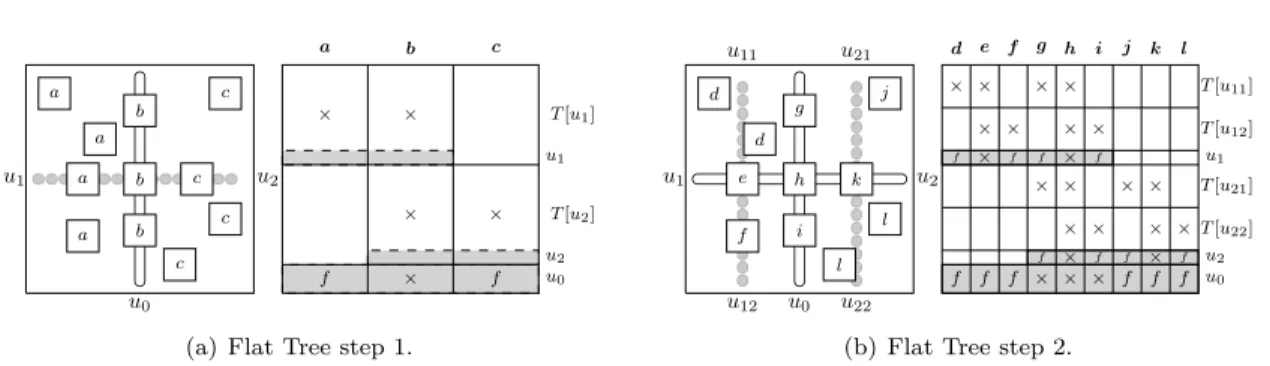
In the example of Section 1, the variables of a separator u are the ones of the corresponding node u in the tree T . We use the same approach to represent a domain: for u ∈ T , the domain associated with u is defined by the subtree rooted at u and is noted T [u]. The set of variables in T [u] corresponds to a subdomain created during the nested dissection algorithm. As an example, the initial 2D domain in Figure 7(a) (left) is T [u0] and its subdomains created by dividing it with u0are T [u1] and T [u2].
In the following, T [u] will equally refer to a subdomain or a subtree. Figure 7 shows several types of RHS with different positions and nonzero structures. For the sake of simplicity, we assume here that the nonzeros in an RHS column correspond to geometrically contiguous nodes in the domain, as represented in Figure 7(a)(left). We also assume a regular domain for which a perfect nested dissection has been performed. For instance, all separators are in the same direction at each level of the tree.
The Flat Tree algorithm relies on the evaluation of the position of each RHS column compared to separators of the nested dissection algorithm. The name Flat Tree comes from the fact that,
u0 u1 a u2 a a a b b b c c c c a b c T [u1] u1 T [u2] u2 u0 × f × × × × f
(a) Flat Tree step 1.
u0 u1 u2 u12 u11 u22 u21 e d d f h g i k j l l d e f g h i j k l T [u11] T [u12] u1 T [u21] T [u22] u2 u0 × f f × × × f × f f × f × f × × × × × × × × × f × f × × f f × × × f × f f
(b) Flat Tree step 2.
Figure 7: A first illustration of the “flat tree” permutation on a 2D domain. In (a) and (b), the figure on the left represents a partitioned 2D domain with different types of RHS, and the one on the right the partial structures of the permuted matrix of RHS. × or f in a rectangle indicate the presence of nonzeros in the corresponding submatrix, parts of the matrix filled in grey are fully dense and blank parts only contain zeros.
given a parent node with two child subtrees in the separator tree T , the algorithm orders first RHS columns included in the left subtree, then RHS columns associated to the parent (because they intersect both subtrees), and finally, RHS columns included in the right subtree. Figure 7(a) shows the first step of the algorithm: it starts with the root separator u0 which divides T = T [u0] into T [u1] and T [u2]. The initial RHS columns may be identified by three different types noted a, b
and c according to their positions and nonzero structures. An RHS column is of type a when its nonzero structure is included in T [u1], c when it is included in T [u2], and b when it is divided by u0. First, we group the RHS according to their type (a, b, or c) with respect to u0which leads to
the creation of submatrices/subsets of RHS columns noted a, b and c. Second, we make sure to place b between a and c. We thus achieve operation reduction by guaranteeing node optimality at u1 and u2: since all RHS in a and b have at least one nonzero in T [u1], u1 belongs to the pruned
tree of all of them, hence the dense area filled in gray in the RHS structure. The same is true for b and c and u2. By permuting B as [a, b, c] ([c, b, a] would also be possible), a and b, and b and c,
are contiguous. Thus, θ(Zu1) = #Zu1, θ(Zu2) = #Zu2 and we have u1− and u2−optimality. The
algorithm proceeds recursively on each newly created submatrix (see Figure 7(b)) to obtain local node optimality. First, d, e, f (resp. j, k, l) form subsets of the RHS of a (resp. c) based on their position/type with respect to u1(resp. u2). Second, thanks to the fact that u1and u2are perfectly
aligned, they can be combined to form a single separator that subdivides the RHS of b into three subsets g, h and i, see Figure 7(b). During this second step, B is permuted as [d, e, f , g, h, i, j, k, l]. The complete permutation is then obtained by applying the algorithm recursively on each subset until the tree is fully processed or the RHS sets contain a single RHS.
This draws the outline of the algorithm introduced with geometrical considerations. The per-mutation fully results from the position of each RHS with respect to separators. However, the algorithm relies on strong assumptions regarding the ordering algorithm and the RHS structure. Without them, it is difficult or impossible to discriminate RHS columns in many cases (for example, when they are separated by several separators). In order to overcome these limitations and enlarge the application field, we now extend these geometrical considerations with a more general approach.
3.2.2 Algebraic approach
Let us consider the columns of B = [B1, B2, . . . , Bm] as an initially unordered set of RHS columns
that we note RB = {B1, B2, . . . , Bm}. A subset of the columns of B is denoted by R ⊂ RB and
a generic element of R (one of the columns Bj ∈ R) is noted r. A permuted submatrix of B can
be expressed as an ordered sequence of RHS columns with square brackets. For two subsets of columns R and R0, [R, R0] denotes a sequence of RHS columns in which the RHS from the subset
R are ordered before those from R0, without the order of the RHS inside R or R0 to be necessarily
defined. We found this framework of RHS sets and subsets simpler and better adapted to formalize our algebraic algorithm than matrix notations with complex index permutations. We recall that T is the tree and that, for r ∈ RB, Tp(r) is the pruned tree of r, as defined in Section 2.1. We now
characterize the geometrical position of a RHS using the notion of pruned layer : for a given depth d in the tree, and for a given RHS r, we define the pruned layer Ld(r) as the set of nodes at depth
d in the pruned tree Tp(r). In the example of Figure 7(a), L1(r) = {u1} for all r ∈ a, L1(r) = {u2}
for all r ∈ c, and L1(r) = {u1, u2} for all r ∈ b. The notion of pruned layers allows to formally
identify sets of RHS with common characteristics in the tree without any geometrical information. This is formalized and generalized by Definition 3.3.
Definition 3.3. Let R ⊂ RB be a set of RHS, and let U be a set of nodes at depth d of the tree
T . We defined R[U ] = {r ∈ R | Ld(r) = U } as the subset of RHS with pruned layer U .
We have for example, see Figure 7: R[{u1}] = a, R[{u2}] = c and R[{u1, u2}] = b at depth d = 1.
The algebraic recursive algorithm is depicted in Algorithm 1. Its arguments are R, a set of RHS and d, the current depth. Initially, d = 0 and R = RB= R[u0], where u0 is the root of the tree T .
At each step of the recursion, the algorithm builds the distinct pruned layers Ui= Ld+1(r) for the
RHS r in R. Then, instead of looking for a permutation σ to minimizeP
u∈Tp(RB)δu× θ(σ(Zu))
(10), it orders the R[Ui] by considering the restriction of problem (10) to R and to nodes at depth
d + 1 of Tp(R). Furthermore, with the assumption that T is balanced, all nodes at a given level of
Tp(R) are of comparable size. δu may thus be assumed constant per level and needs not be taken
into account in our minimization problem. The algorithm is thus a greedy top-down algorithm, where at each step a local optimization problem is solved. This way, priority is given to the top layers of the tree, which are in general more critical because factor matrices are larger.
Algorithm 1 Flat Tree procedure Flattree(R, d)
1) Build the set of children C(R)
1.1) Identify the distinct pruned layers (pruned layer = set of nodes) U ← ∅
for all r ∈ R do U ← U ∪ {Ld+1(r)}
end for
1.2) C(R) = {R[U ] | U ∈ U }
2) Order children C(R) as [R[U1], . . . , R[U#C(R)]]:
return [Flattree(R[U1], d + 1),. . .,Flattree(R[U#C(R)], d + 1)]
The recursive structure of the algorithm can be represented by a recursion tree Trecdefined as
follows: each node R of Trecrepresents a set of RHS, C(R) denotes the set of children of R and the
root is RB. By construction of Algorithm 1, C(R) is a partition of R, i.e., R = ˙SR0∈C(R)R0(disjoint
union). Note that all r ∈ R such that Ld+1(r) = ∅ belong to R[∅], which is also included in C(R). In
this special case, R[∅] can be added at either extremity of the current sequence without introducing extra computation and the recursion stops for those RHS, as will be illustrated in Example 3.3.
With this construction, each leaf of Treccontains RHS with indistinguishable nonzero structures,
and keeping them contiguous in the final permutation avoids introducing extra computations. As-suming that for each R ∈ Trec the children C(R) are ordered, this induces an ordering of all the
leaves of the tree, which defines the final RHS sequence. We now explain how the set of children C(R) is built and ordered at each step:
1) Building the set of children The set of children of R in the recursion tree is built by first
identifying the pruned layers U of all RHS r ∈ R. The different pruned layers are stored in U and we have for example (Figure 7, first step of the algorithm), U = {{u1}, {u2}, {u1, u2}}. Using
Definition 3.3, we then define C(R) = {R[U ] | U ∈ U }, which forms a partition of R. One important property is that all r ∈ R[U ] have the same nonzero structure at the corresponding layer so that numbering them contiguously prevent the introduction of extra computation.
2) Ordering the children At each depth d of the recursion, the ordering of the children
results from the resolution of the local optimization problem consisting in finding a sequence [R[U1], . . . , R[U#C(R)]] such that the size of the intervals is minimized for all nodes u at depth d + 1 of the pruned tree Tp(R). As mentioned earlier, when solving this local optimization problem,
the RHS order inside each R[Ui] has no impact on the size of the intervals (it will only impact lower
levels). For any node u in Tp(R) such that depth(u) = d + 1, the size of the interval is then:
θ(Zu|R) = max(Zu|R) − min(Zu|R) + 1 = imax(u)
X
i=imin(u)
#R[Ui],
where Zu|R is the set of permuted indices representing the active columns restricted to R, and
imin(u) = min{i ∈ {1, . . . , #C(R)} | u ∈ Ui} (resp. imax(u) = max{i ∈ {1, . . . , #C(R)} | u ∈ Ui})
is the first (resp. last) index i such that u ∈ Ui.
Proof. In the sequence [R[U1], . . . , R[U#C(R)]], min(Zu|R) (resp. max(Zu|R)) corresponds to the
index of the first (resp. last) column in R[Uimin] (resp. R[Uimax]). Since all columns from R[Uimin]
to R[Uimax] are numbered consecutively, we have the desired result.
Finally, our local problem consists in minimizing the local cost function (sum of the interval sizes for each node at depth d + 1):
cost([R[U1], . . . , R[U#C(R)]]) = X u∈Tp(R) depth(u)=d+1 imax(u) X
i=imin(u)
#R[Ui] (11)
To build the ordered sequence [R[U1], . . . , R[U#C(R)]], we use a greedy algorithm that starts
randomly in C(R) at the position that minimizes (11) on the current sequence. To do so, we simply start from one extremity of the sequence of size k − 1 and compute (11) for the new sequence of size k for each possible position 0 . . . k; if several positions lead to the same minimal cost, the first one encountered is chosen. In case u−optimality is obtained for each node u considered, then the permutation is said to be perfect and the cost function is minimal, locally inducing no extra operations on those nodes.
R[u0]
d = 0
R[u1] R[u1u2] R[u2]
d = 1
R[u11] R[u11u12] R[u12] ∗ R[u21] R[u21u22] R[u22]
d = 2
Figure 8: Representation of a layered sequence built by the Flat Tree algorithm on a binary tree. Sets with empty pruned layers have not been represented but could be added at the extremity of the concerned sequence (e.g., right after R[u2] for a RHS included in u0). With the geometric
assumptions corresponding to Figure 7, one would have * = R[u11u21], R[u11u12u21u22], R[u12u22].
Without such assumptions, the sequence * is more complex.
Figure 8 shows the recursive structure of the RHS sequence after applying the algorithm on a binary tree. We refer to this representation as the layered sequence. For simplicity, the notation for pruned layers has been reduced from, e.g., {u1} to u1, and from {u1, u2} to u1u2. From the recursion
tree point of view, R[u1], R[u1u2], R[u2] are the children of R[u0] in Trec, R[u11], R[u11u12], R[u12]
the ones of R[u1], etc.
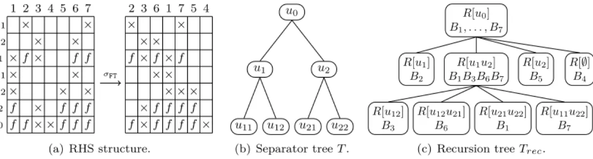
× × × f f f f × × × × × × × f f × f × f f × f × f f u0 u2 u22 u21 u1 u12 u11 1 2 3 4 5 6 7 σFT f f × × × × × × f × f f × × × f f × f × f f × f f × 2 3 6 1 7 5 4 (a) RHS structure. u0 u2 u22 u21 u1 u12 u11 (b) Separator tree T . R[u0] B1, . . . , B7 R[u1u2] B1B3B6B7 R[u11u22] B7 R[u21u22] B1 R[u12u21] B6 R[u12] B3 R[u1] B2 R[u2] B5 R[∅] B4
(c) Recursion tree Trec.
Figure 9: Illustration of the algebraic Flat Tree algorithm on a set of 7 RHS.
Example 3.3. Let B = [B1, B2, B3, B4, B5, B6, B7] be a RHS matrix with the structure presented
in Figure 9(a). Although we still use a binary tree, we make no assumption on the RHS structure, on the domain, or on the ordering. We have RB= R[u0] = {B1, B2, B3, B4, B5, B6, B7}. At depth
1, the set of pruned layers corresponding to R[u0] is U = {u1, u1u2, u2, ∅}, with the RHS partition
composed of the sets R[u1], R[u2], R[u1u2] and R[∅]. Then, C(R[u0]) = {R[u1], R[u1u2], R[u2], R[∅]}
and the recursion tree shown in Figure 9(c) is built from top to bottom. As can be seen in the non-permuted RHS structure, R[∅] = B4 at depth 1 induces extra operations at nodes
place it last, and the ordered sequence obtained by the algorithm is [R[u1], R[u1u2], R[u2], R[∅]]
([R[u2], R[u1u2], R[u1], R[∅]] is also possible). A recursive call is done on each of the identified sets.
We only focus on R = R[u1u2] since R[u1], R[u2] and R[∅] contain a single RHS which needs not
be further ordered. At this stage, the set of pruned layers is U = {u21u22, u12, u12u21, u11u22}. It
appears that the sequence [R[U1], R[U2], R[U3], R[U4]], where U1= u12, U2= u12u21, U3= u21u22,
and U4 = u11u22 is a perfect sequence which gives local optimality. However, taking the problem
globally, we see that θ(Zu11) 6= #Zu11 with the final sequence [B2, B3, B6, B1, B7, B5, B4].
The algebraic algorithm simplifies the assumptions that were made in the geometrical one. The nonzeros of each RHS no longer need to be geometrically localized, and we can address irregular problems and orderings that yield non binary trees. We compared both approaches on problems H0, H3, 5Hz and 7Hz from Table 2 and observed, even with nested dissection, an average 7% gain on ∆ with the algebraic approach, which we will use in all our experiments. Nevertheless, computations on explicit zeros (for example zero rows in column f and subdomain T [u11] in Figure 7(b)), may
still occur. This will also be illustrated in Section 5, where ∆(B, σFT) is 39% larger than ∆min(B),
in the worst case. A Blocking algorithm is now introduced to further reduce ∆(B, σFT).
4
Toward a minimal number of operations using blocks
In this section, we identify the causes of the remaining extra operations and provide an efficient blocking algorithm to reduce them efficiently while creating a small number of blocks. The algorithm relies on a property of independence of right-hand sides that is first illustrated, and then formalized.
4.1
Objectives and first illustration of independence property
The use of blocking techniques may fulfill different objectives. In terms of operation count, op-timality (∆min(B)) is obtained when processing the columns of B one by one, which implies the
creation of m blocks. However, this requires processing the tree m times and will typically lead to a poor arithmetic intensity (and likely a poor performance). On the other hand, the algorithms of Section 3 only use one block, which allows a higher arithmetic intensity but leads to extra op-erations. In the dense case, blocks are also often used to improve the arithmetic intensity. In the sparse RHS case, blocking techniques with regular blocks of columns have been associated to tree pruning to either limit the access to the factors [3], or limit the number of operations [18]. They were either based on a preordering of the columns or on hypergraph models. In this section, to give as much flexibility as possible to the underlying algorithms and avoid unnecessary constraints, our objective is to create a minimal number of (possibly large) blocks while reducing the number of extra operations by a given amount. In particular, we allow blocks to be irregular and assume node intervals are exploited within each block.
On the one hand, in the same way as variables in two different domains are independent, two RHS or two sets of RHS included in two different domains exhibit interesting properties, as can be observed for sets a ∈ T [u1] and c ∈ T [u2] from Figure 7(a). It implies that no extra operations
are introduced between them: ∆([a, c]) = ∆(a) + ∆(c). We say that a and c are independent sets and can thus be associated together. On the other hand, a set of RHS intersecting a separator (such as set b) exhibits some zeros and nonzeros in rows common to their adjacent RHS sets (a and c) which will likely introduce extra computation. For example, one can see in Figure 7(b) that ∆([a, b]) = ∆([d, e, f , g, h, i]) > ∆([d, e, f ]) + ∆([g, h, i]) = ∆(a) + ∆(b) and that ∆([a, b, c]) >
∆(a) + ∆(b) + ∆(c). We say that b is a set of problematic RHS. Another example is the one of Figure 6 (right), where extracting the problematic RHS B1 and B5 from [B4, B2, B1, B5, B6, B3]
suppresses all extra operations: ∆([B4, B2, B6, B3]) + ∆([B1, B5]) = ∆min= 1056.
To give further intuition on the Blocking algorithm, consider the RHS structure of Figure 7(b). Problematic RHS e and k in [d, e, f , j, k, l] can be extracted to form two blocks, or groups, [e, k] and [d, f , j, l]. The situation is slightly more complicated for [g, h, i], where h indeed intersects two separators, u1and u2. In this case, h should be extracted to form the groups [g, i] and [h]. We note
that the amount of extra operations will likely be much larger when the separator intersected is high in the tree. Situations where no assumption on the RHS structure is made are more complicated and require a more general approach. For this, we formalize the notion of independence, which will be the basis for our blocking algorithm.
4.2
Algebraic formalization and first blocking algorithm
In this section, we give a first version of the Blocking algorithm. It is based on a sufficient condition allowing to group together sets of RHS without introducing extra computation. We assume the matrix B to be flat tree ordered and the recursion tree Trec to be built and ordered. Using the
notations of Definition 3.3, we first give an algebraic definition of the independence property between two sets of RHS:
Definition 4.1. Let U1, U2 be two sets of nodes at a given depth of a tree T , and let R[U1], R[U2]
be the corresponding sets of RHS. R[U1], R[U2] are said to be independent if and only if U1∩U2= ∅.
With Definition 4.1, we are able to formally identify independent sets and we will show formally why they can be associated together. For example, take a = R[u1] and c = R[u2] from Figure 7(a), R[u1] and R[u2] are independent and ∆([R[u1], R[u2]]) = ∆(R[u1]) + ∆(R[u2]). On the contrary,
when R[U1], . . . , R[Un] are not pairwise independent, the objective is to group together independent
sets of RHS, while forming as few groups as possible. In terms of graphs, this problem is equivalent to a classical coloring problem, where R[U1], . . . , R[Un] are the vertices and an edge exists between
R[Ui] and R[Uj] if and only if Ui ∩ Uj 6= ∅. Several heuristics exist for this problem, and each
color will correspond to one group. The Blocking algorithm as depicted in Figure 10 consists of a
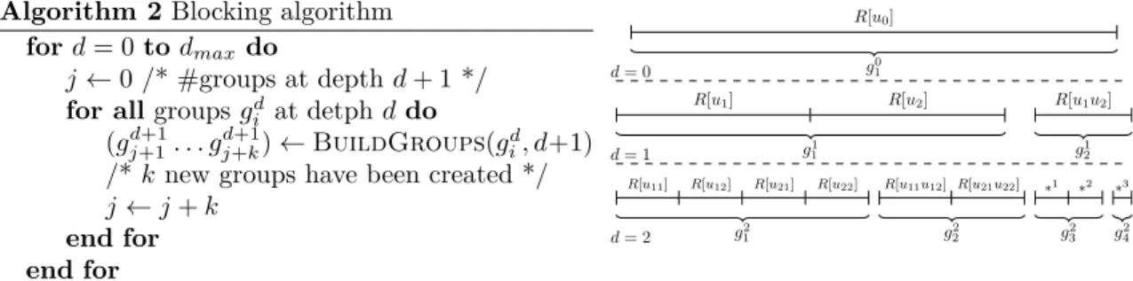
Algorithm 2 Blocking algorithm
for d = 0 to dmaxdo
j ← 0 /* #groups at depth d + 1 */
for all groups gd
i at detph d do
(gj+1d+1. . . gd+1j+k) ← BuildGroups(gd i, d+1)
/* k new groups have been created */ j ← j + k end for end for R[u0] g0 1 d = 0
R[u1] R[u2] R[u1u2]
g1
1 g21
d = 1
R[u11] R[u12] R[u21] R[u22]
g2 1 R[u11u12] R[u21u22] g2 2 ∗1 ∗2 g2 3 ∗3 g2 4 d = 2
Figure 10: A first version of the Blocking algorithm (left). It is illustrated (right) on the layered sequence of Figure 8. With the geometric assumptions of Figure 7, ∗1= R[u
11u21], ∗2= R[u12u22],
and ∗3= R[u
11u12u21u22].
procedure BuildGroups is called. Notice that any group gd
i verifies the following properties: (i)
gd
i can be represented by a sequence [R[U1], . . . , R[Un]], and (ii) the sequence respects the flat tree
order of Trec. Then, BuildGroups(gid, d + 1) first builds the sets of RHS at depth d + 1, which
are exactly the children of the R[Uj] ∈ gdi in Trec. Second, BuildGroups(gdi, d + 1) solves the
aforementioned coloring problem on these RHS sets and builds the k groups (gj+1d+1, . . . , gj+kd+1). In the example of Figure 10(right), there is initially a single group g0
1 = [R[u0]] with one
set of RHS. This group may be expressed as the ordered sequence [R[u1]R[u1u2]R[u2]], since C(R[u0]) = {R[u1], R[u1u2], R[u2]}. g01 does not satisfy the independence property at depth 1
because u1∩ u1u2 6= ∅ or u2∩ u1u2 6= ∅. BuildGroups(g10, 1) yields g11 = [R[u1], R[u2]] and g12 = [R[u1u2]]. The algorithm proceeds on each group until a maximal depth dmax is reached:
(g21, g22) = BuildGroups(g11, 2), (g23, g24) = BuildGroups(g12, 2), etc. To illustrate the interest of
property (ii) on groups, let us take sets d = R[u11], f = R[u12], j = R[u21] and l = R[u22] from
Figure 7(b). One can see that ∆([d, f , j, l]) = ∆(d) + ∆(f ) + ∆(j) + ∆(l) < ∆([d, j, f , l]). Com-pared to [d, f , j, l] which respects the global flat tree ordering and ensures u1- and u2-optimality,
[d, j, f , l] does not and thus increases θ(Zu1) and θ(Zu2).
Furthermore, Algorithm 2 ensures the following property, which shows that the independent sets of RHS grouped together do not introduce extra operations.
Property 4.1. For any group gd= [R[U
1], . . . , R[Un]] created through Algorithm 2 at depth d, we
have ∆([R[U1], . . . , R[Un]]) =P n
i=1∆(R[Ui]).
Proof. For d ≥ 1, let gd= [R[Uid]i=1,...,nd] be a group at depth d created through Algorithm 2 (we
use superscripts d in this proof to indicate the depth without ambiguity). Let us split nodes above (A) and below (B) layer d in the pruned tree Tp(gd). The number of operations to process gd is:
∆(gd) = X u∈Tp(gd) δu× θ(Zu|gd) = ∆A z }| { X u∈A δu× θ(Zu|gd) + ∆B z }| { X u∈B δu× θ(Zu|gd), (12)
where A = {u ∈ Tp(gd) | depth(u) < d} and B = {u ∈ Tp(gd) | depth(u) ≥ d}.
(i) We first consider the term ∆B. Let Bi = {u ∈ Tp(R[Uid]) | depth(u) ≥ d}. Thanks to the
independence property of the R[Uid] forming gd, the pruned layers Uid in T are disjoint and since T is a tree, we have Bi∩ Bj = ∅ for all i 6= j. Hence, B = ˙S
nd
i=1Bi, where ˙S denotes the disjoint
union. Therefore, ∆B= X u∈S˙nd i=1Bi δu× θ(Zu|[R[Ud j]j=1,...nd]) = nd X i=1 X u∈Bi δu× θ(Zu|[R[Ud j]j=1,...nd]).
We recall that a RHS r is said to be active at node u if u ∈ Tp(r). In the inner sum, the only possible
active RHS in Bi are the ones that belong to R[Uid] (independence of the R[Ujd]), so that for all
u ∈ Bi, we have θ(Zu|[R[Ud
i]i=1,...nd]) = θ(Zu|R[Uid]). Therefore, ∆B =
Pnd
i=1
P
u∈Biδu× θ(Zu|R[Uid]).
(ii) We now consider the term ∆A. Similarly to (i), we define Ai= {u ∈ Tp(R[Uid]) | depth(u) < d}.
We have A =Snd
i=1Ai but the union is no longer disjoint. Let Trec(gd) be the restriction to gd of
the recursion tree Trecassociated to the flat-tree algorithm applied to RB(see Section 3.2.2 for the
are not part of gd, then by pruning all empty nodes. We also restrict Definition 3.3 to gdand thus
note R[U ] = {r ∈ gd| L
d(r) = U }. In particular, the root of Trec(gd) is R[u0] = gd.
By construction of Algorithm 2 (Figure 10), we know that any layer at depth d0 < d of the group gd consists of independent sets R[Ujd0] of RHS. Therefore, ∀u ∈ A, ∃!R[U ] ∈ Trec(gd) such
that u ∈ U . This means that the only active columns at node u are those in this unique R[U ] and, since the RHS in R[U ] are all contiguous in gd thanks to the global flat tree ordering, we have θ(Zu|R[U ]) = θ(Zu|gd) = #R[U ].
Furthermore, by construction of the recursion tree (children nodes form a partition of each parent node), the RHS in R[U ] are the ones in the disjoint union of R[Ud
i] ⊂ R[U ], the sets of right-hand
sides at layer d that are descendants of R[U ] in Trec(gd). Therefore, #R[U ] =PR[Ud
i]⊂R[U ]
#R[Ud i].
Furthermore, since the R[Uid] such that R[Uid] ⊂ R[U ] are contiguous sets in gd and are all active at node u, we also have θ(Zu|R[Ud
i]) = #R[U d i]. It follows: θ(Zu|gd) = X R[Ud i]⊂R[U ] θ(Zu|R[Ud i]).
We define ξi(u) = 1 if R[Uid] ⊂ R[U ] (with R[U ] derived from u as explained above), and
ξi(u) = 0 otherwise. The condition R[Uid] ⊂ R[U ] means that u is an ancestor of Uid nodes in T .
Thus, ξi(u) = 1 for u ∈ Ai and ξi(u) = 0 for u /∈ Ai. We can thus writePR[Ud
i]⊂R[U ]θ(Zu|R[U
d i]) =
Pnd
i=1ξi(u)θ(Zu|R[Ui]) and redefine ∆Aas:
∆A= X u∈A δu× θ(Zu|gd) = X u∈A δu× nd X i=1 ξi(u)θ(Zu|R[Ud i]) = nd X i=1 X u∈A δu× ξi(u)θ(Zu|R[Ud i]) = nd X i=1 X u∈Ai δu× θ(Zu|R[Ud i]).
Joining the terms ∆A and ∆B, we finally have:
∆(gd) = ∆A+ ∆B = nd X i=1 X u∈Bi δu× θ(Zu|R[Ui]) + nd X i=1 X u∈Ai δu× θ(Zu|R[Ui]) = nd X i=1 ∆(R[Ui])
Interestingly, Property 4.1 can be used to prove, in the case of a single nonzero per RHS, the optimality of the Flat Tree permutation.
Corollary 4.1. Let RB be the initial set of RHS such that ∀r ∈ RB, #Vr= 1. Then the Flat Tree
permutation is optimal: ∆(RB) = ∆min(RB).
Proof. Since ∀r ∈ RB, #Vr= 1, Tp(r) is a branch of T . Indeed, Vris a singleton and Tp(r) is built
through the Flat Tree algorithm will be represented by a pruned layer U containing a single node u. Thus, at each step of the algorithm, the RHS sets identified by the Flat Tree algorithm are all independent from each other. In case Algorithm 2 is applied, a unique group RB is then kept until
the bottom of the tree. Blocking is thus not needed and Property 4.1 applies at each level of the flat tree recursion. ∆(RB) is thus equal to the sum of the ∆(R[U ]) for all leaves R[U ] of the recursion
tree Trec. Since ∆(R[U ]) = ∆min(R[U ]) on those leaves (all RHS in R[U ] involve the exact same
nodes and operations), we conclude that ∆(RB) = ∆min(RB).
This proof is independent of the specific ordering of the children at step 2 of Algorithm 1. The corollary is therefore more general: any recursive top-down ordering based on keeping together at each layer the RHS with an identical pruned layer is optimal, as long as the pruned layers identified at each layer are independent.
R[u1] R[u2]
g1 1
d = 1
R[u11] R[u12] R[u21] R[u22]
g2 1 R[u11u12] R[u21u22] g2 2 d = 2 R[u1] R[u2] g1 1 d = 1
R[u11] R[u12] R[u21u22]
g2 1
R[u21] R[u22] R[u11u12]
g2 2
d = 2
Figure 11: Two strategies to build groups: CritPathBuildGroups (left) and RegBuildGroups (right).
Back to the BuildGroups function and the coloring problem, we mention that the solution may not be unique. Even on the simple example of Figure 10, there are several ways to define groups, as shown in Figure 11 for g11: both strategies satisfy the independence property and minimize the number of groups. The CritPathBuildGroups strategy tends to create a large group g21 and
a smaller one, g22. In each group the computations on the tree nodes are expected to be well
balanced because all branches of the tree rooted at u0might be covered by the RHS (assuming thus
a reasonably balanced RHS distribution over the tree). The choice of CritPathBuildGroups can be driven by tree parallelism considerations, namely, the limitation of the sum of the operation count on the critical paths of all groups. The RegBuildGroups strategy tends to balance the sizes of the groups but may create more unbalance regarding the distribution of work over the tree. We note that for a given depth, the application of BuildGroups on all groups may lead to a too rapid and unnecessary increase of the number of groups. Furthermore, the enforcement of the independence property during the BuildGroups operation may require the creation of more than two groups. In the next section we add features to minimize the number of groups created using greedy heuristics and propose our final version of the Blocking algorithm.
4.3
A greedy approach to minimize the number of groups
The final greedy blocking algorithm is given by Algorithm 3. Compared to Algorithm 2, it adds the group selection, limits the number of groups during BuildGroups to two, and stops when a given tolerance on the amount of extra operations is reached.
First, instead of stepping into each group, as in Algorithm 2, the group selection consists in choosing among the current groups the one responsible for most extra computation, that is, the