Simultaneous measurement of the phase noise on all optical modes of a mode-locked laser

DOI: 10.1007/s00340-007-2728-1 Lasers and Optics

a. schlatter s.c. zeller r. paschotta∗ u. kelleru

Simultaneous measurement of the phase noise

on all optical modes of a mode-locked laser

Received: 29 May 2007

Published online: 1 August 2007 • © Springer-Verlag 2007 ABSTRACT We propose and experimentally demonstrate a method to simultaneously measure the relative phase noise of all modes of two mode-locked lasers. The method is based on the numerical analysis of a beat note of two lasers with slightly different pulse repetition rates. We carefully analyze and exper-imentally demonstrate the potential of this method. Compared to other methods, it has the unique advantage that it provides access to correlations of the phases of different modes. PACS42.60.Mi; 42.60.Fc

1 Introduction

Mode-locked lasers emit regular pulse trains, the optical spectra of which are equidistant frequency combs. Particularly the recent advances in the measurement and control of the carrier-envelope offset frequency [1] have greatly expanded the range of possible applications of such frequency combs, enabling e.g., extremely precise optical frequency measurements in a wide spectral region, and phase-coherent links between microwave and optical frequency standards, as required for the next generation of atomic clocks. In many cases, the noise properties of frequency combs are important, often even limiting factors for appli-cations. Therefore, the investigation of such noise properties is vital for a large field within the science and technology of photonics.

The so far probably most often considered noise property of pulse trains is the timing jitter, but the increasing use of co-herent effects (such as beat note measurements) draws more and more attention to phase noise. Comparing to continuous-wave single-frequency lasers, in the context of mode-locked lasers, we are dealing with a significant (or sometimes even very large) number of lines in the spectrum. Relevant quanti-ties concern not only the magnitude of noise in all these lines, but also possible correlations between the phase fluctuations in different lines. While theoretical expectations for such phe-nomena have recently been discussed in detail [2], and the

u Fax: +41 44 633 10 59, E-mail: keller@phys.ethz.ch

∗_{New address: R.P. left ETH in June 2005 to RP Photonics Consulting}

GmbH, Zurich, Switzerland

relation of noise in all the spectral lines to pulse timing noise and the noise of the carrier-envelope offset has been clarified in the same paper, the experimentally explored domain is so far significantly smaller. Extensive investigations of timing jitter with various methods (see e.g. [3–6]) are found in the lit-erature. All phase noise measurements on mode-locked lasers which have been reported so far to our best knowledge refer either to the phase noise in a single line (retrieved e.g., via a beat note measurement with a single-frequency laser [7, 8]), or rarely to a few lines, or to some average over all lines (obtained by beating the outputs of two synchronized mode-locked lasers [9]). To obtain phase noise in multiple lines, one may either subsequently apply single-line methods to dif-ferent lines [10] (but then not obtaining any information on correlations), or simultaneously apply such a method to mul-tiple lines, which however introduces tight practical limits concerning the number of accessible lines. In this article we describe a measurement method which allows one to simul-taneously retrieve the phase noise of dozens of lines, together with their correlations and related quantities like timing jitter and noise of the carrier-envelope offset, while requiring only a very simple measurement setup.

2 Description of the measurement technique

To measure the relative phase noise of two lasers, we record beat notes using a simple setup as depicted in Fig. 1. The setup contains two mode-locked lasers, the phase noise of which is to be compared. Both lasers operate at a wavelength of 1342 nm and with pulse repetition rates near 5 GHz. Their fiber-coupled outputs are combined with a standard fiber cou-pler after aligning the polarization directions with fiber polar-ization controllers. An InGaAs p–i–n photodiode (type ETX 100 from JDSU) with a 3-dB bandwidth of 1 GHz records a beat note, which is then digitized after electronic low-pass filtering in order to remove unwanted signals and to avoid aliasing effects in the digitizer.

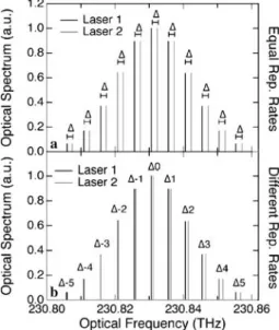
Recording beat notes of mode-locked lasers involves some aspects which do not occur for single-frequency lasers. For synchronized pulse trains (i.e., equal repetition rates), the spectra of both lasers are frequency combs with equal spacing but (in general) some offset due to the difference of the carrier-envelope offset frequencies (see Fig. 2a). A beat note is then only recorded if the pulses of both lasers temporally overlap at the detector. In that case, the single-tone beat signal contains

FIGURE 1 Experimental setup for our phase noise measurements. ml= mode-locked, PC = polarization control, PD = photodiode. The photo-diode signals are low-pass filtered and digitally recorded

contributions from all mode pairs. The lowest beat frequency corresponds to the difference of the carrier-envelope offset frequencies of the two lasers and lies in the range from zero to half the pulse repetition rate.

In the measurement technique described here, we use slightly detuned repetition rates. Therefore, the frequency combs have different spacing, and there are separate beat notes for each mode pair (Fig. 2b). The recorded signal con-tains separate beat components from all different pairs of lines from the two lasers, because the line spacings (equal to the pulse repetition rates) are slightly different. The electronic low-pass filter eliminates all beat components with higher frequencies, resulting e.g., from different lines of one laser, and the obtained signal can later be numerically decomposed into the separate beat components. We discuss in detail the evaluation procedure in Sect. 3 and various limitations and re-quirements in Sect. 4.

In the time domain, we obtain a signal as shown in Fig. 3: Most of the time the pulses do not overlap and the signal sim-ply corresponds to the sum of the average powers of the two lasers. As the repetition rates are different, the pulses will

FIGURE 2 Illustration of the optical spectra of two mode-locked lasers. (a) Equal rep. rates: All line pairs add up to generate a single beat note with frequency∆ = ∆ fCEO. (b) Slightly different rep. rates: Each mode pair has a different offset and generates a unique beat frequency∆i

FIGURE 3 Short section of a measured beat signal. Every time the pulses overlap, an alternating pattern of constructive and destructive interference is obtained. The smaller pattern indicates a small satellite pulse of one laser

overlap from time to time, generating an interference signal where constructive or destructive superposition of the pulses can occur, depending on the relative phase.

3 Evaluation procedure

After we have recorded the beat signal, we can numerically extract the phase and amplitude noise, as well as information on noise correlations. As a first step, we need to separate the beat spectrum (see Fig. 4) into individual beat lines. These are subsequently analyzed one by one.

3.1 Beat note separation

For separating the different beat notes, we essen-tially only need to split the Fourier spectrum of the recorded signal, as obtained with a fast Fourier transform (FFT) algo-rithm, into suitable slices. Ideally, each beat note would be centered in its slice, and its sidebands contain the informa-tion on amplitude and phase noise. The exact slicing posiinforma-tions are actually not important, since no information is lost in this process. For each slice, we do a reverse FFT, and from the observed linear drift of the recorded phase we retrieve a fre-quency offset. By adding this frefre-quency offset to the center frequency of the slice, we obtain the exact line frequency. Fol-lowing such a procedure, we have found the line frequencies to be equidistant within the spectral resolution of the measure-ment. The standard deviation of the calculated line frequen-cies relative to an exactly equidistant grid is typically around 30%of the frequency bin width of the spectrum. In absolute terms, we found an rms deviation of only 4 Hz over a range of optical frequencies of 140 GHz (28 optical modes).

FIGURE 4 Power spectral density of a measured beat signal (black). The noise background is limited by noise of the sampling card (gray)

3.2 Noise evaluation

In the following, we explain how to calculate phase and amplitude noise from the spectrum of each extracted beat line. The spectral separation as discussed above results in one spectral slice for each beat note. We can now limit the width of each slice according to the maximum noise frequency of in-terest. We also shift the zero point of the frequency axis to the peak position, but of course remember the applied frequency shift so that we can always retrieve the actual frequency. The reverse FFT then results in a slowly varying time domain pha-sor, the amplitude of which is proportional to the product of the optical amplitudes. Its phase corresponds to the phase difference of the two generating optical modes, apart from a linear term related to the frequency difference and applied frequency shift.

This procedure is applied to all lines of the beat spectrum, so that we retrieve all the phasors for the same time interval of the measurement. It is, thus, possible to analyze the data for correlations. As a simple example, consider a situation where the cavity length of one of the lasers changes suddenly. This will modify all line frequencies of this laser, with a “fix point” in the “rubber-band model” of [11] near zero frequency. We, thus, expect an additional linear phase drift of all lines, with the rate of change proportional to the optical frequency. With our method we can experimentally distinguish this situation from another one where e.g., the fix point would be at the cen-ter of the optical spectrum, so that changes of the repetition rate would lead to drifts of the phases of high and low fre-quency beat components in opposite directions.

From all the obtained time-dependent quantities (e.g., line amplitudes and phases), we can subsequently calculate noise spectra by applying an FFT after multiplying the data with a suitable window function.

4 Discussion of the potential of the method

In the following we discuss the limitations of the proposed measurement technique, together with the require-ments for the choice of the repetition rate difference. We show that the method has a valuable potential for accurate phase and amplitude noise measurements particularly for lasers with a not too high duty cycle, i.e., with a pulse duration which is not too many orders of magnitude below the pulse spacing. Basic limitations of accuracy arise from noise in the photo-detectors (Sect. 4.1) and from digital sampling (Sect. 4.2), but these factors can be strongly influenced by the choice of components and of the sampling parameters. In Sect. 4.3 we discuss coupling of intensity to phase noise, and in Sect. 4.4 we show how the choice of repetition rate difference affects the range of measurable noise frequencies, and the spurious-free dynamic range. A summary is given in Sect. 4.5.

A photodiode generates a current which is proportional to the incident optical power within certain limits for the pulse peak power or the average power, depending on the situation. In our case, the peak power limit sets the limit for the aver-age current we can obtain from the detector and therefore the amplitudes of the beat lines. Usually, the photodiode cur-rent is then converted to a voltage over some impedance for measurement. Because most sources of measurement noise

are independent of signal strength, this results in a limited signal-to-noise ratio, particularly for lasers with many spec-tral lines (i.e., a low duty cycle) and in any case for the weaker lines in the beat spectrum. Depending on the signal-to-noise ratio of each line, this will cause some phase noise as well as intensity noise background. The main sources of measurement noise are shot noise, thermal electronic noise, and digitizer noise, which we will discuss in the follow-ing. The discussion is based on the one of [6], using two-sided power densities. Note that the engineering disciplines usually use one-sided power densities, which are two times larger.

4.1 Noise from detection electronics

Obviously, the photodetection noise leads to a basic limitation of the sensitivity of the proposed measure-ment technique. Basically we are dealing with two different kinds of noise: Electronic noise, which arises partly from ther-mal noise in electronic components, and shot noise, which is a quantum effect. A typical kind of photodetector consists simply of a reverse-biased photodiode, the output current of which is converted to a voltage over the input impedance of the electronics it is attached to, usually R= 50 Ω. If this is purely resistive, it contributes thermal noise with a two-sided power density

SδU( f) = 2kBTR (1)

of the current. T is the temperature (typically room ture) at which the electronics are operated. At room tempera-ture we find a power spectral density of 4× 10−19V2/Hz. If an electronic preamplifier is used to boost the power of the resulting signal, the relative intensity noise in the amplified signal is increased by the noise figure of the amplifier, which is typically a few dB.

We can also have the influence of shot noise, leading to a detected voltage noise with a power density

S_δU( f) = e ¯IR2. (2)

Note that a high average current is desirable. Although this increases the noise power density, it still improves the signal-to-noise ratio because the signal power is proportional to ¯I2_. For an average current of, e.g., 2 mA, we obtain a noise back-ground at 8× 10−19V2_{/Hz. As this type of noise is} propor-tional to the current, it can dominate over thermal noise for high measured voltages. The average voltage ¯Ucwhere both contributions are equal is

¯Uc= ¯IcR= 2kBT

e ≈ 50 mV . (3)

Note that pulse trains with low repetition rates and short pulses have a higher ratio of peak to average power (lower duty cycle), so that lower detected average powers are re-quired to avoid detector saturation. In that case, thermal noise can easily dominate over shot noise, and the signal power is strongly reduced. This can quickly lead to an unsatisfactory signal-to-noise ratio.

4.2 Noise from digital sampling

Our method involves digital sampling of data, which unavoidably leads to sampling errors. Additionally, jit-ter of the sampling clock results in apparent phase noise of the measured signal. However, a suitable choice of the sampling parameters allows one to achieve a rather low noise level. 4.2.1 Sampling errors. According to [6], the sampling of a signal with an n-bit digitizer, a full-scale voltage Umax, and a time resolution∆t leads to an approximately white noise floor with power density

SδU( f) = 1 122

−2n_U2

max∆t . (4)

This shows that the bit resolution is rather important: Each ad-ditional bit reduces the noise level by 6 dB; the same could be achieved only with a fourfold increase of the sampling rate.

Note that the best signal-to-noise ratio – and therefore the lowest possible phase noise floor – is achieved when the signal uses the full range of input voltages. In practice one usually requires some margin to avoid clipping of the signal. Also, real digitizers often have a significantly higher noise floor than theoretically possible due to analog noise affecting the input signal.

We can reduce this noise floor by increasing the sampling rate fs= 1/∆t. On the other hand, the lowest measurable noise frequency is 1/(N∆t) = fs/N, so that a high sampling rate increases the required number N of samples for a given lower noise frequency. A more effective way to lower the noise floor is to increase n, the number of bits.

As a numerical example, assume a sampling resolution of 12 bits, an input range of 200 mV, and a sampling rate of 100 MHz. This leads to an estimated noise floor of≈ 2 × 10−18V2_/Hz.

4.2.2 Sampling clock jitter. When digitizing a sine wave with a frequencyω0, we record values

y(n) = sin(ω0t(n)) ,

with n being the sample number. With a sinusoidally fluctuat-ing samplfluctuat-ing clock we have

t(n) = ∆t n + δt sin(ωm∆t n) , and therefore

y(n) = sin(ω0∆t n + ω0δt sin(ωm∆t n)) .

This is a sine wave with sinusoidal phase modulation with an amplitudeδϕ = ω0δt. From this we derive that sampling clock timing jitter leads to an apparent phase noise power density of

Sδϕ( f) = ω20Sδt,clock( f) . (5)

Note that the apparent phase noise depends on the fre-quency of the sampled signal. The sampling clock jitter of a digitizer can usually be found in its specification. Otherwise, it needs to be measured. The digitizer we used

in our experiments (National Instruments NI5122) is spec-ified to introduce an apparent phase noise on a 10-MHz sine wave that is less than(−100, −120, −130) dBc/Hz at a noise frequency of (100, 103_{, 10 × 10}3_{) Hz, respectively.} At the highest possible frequency the digitizer is able to re-solve (50 MHz) the noise background rises according to (5) to(−86, −104, −116) dBc/Hz.

4.3 Coupling of intensity noise to phase noise

In any case, AM-PM conversion requires some kind of nonlinearity. For operation at low enough optical power levels, the photodetectors are operating in the linear regime, avoiding any AM-PM coupling. However, there is a need to maximize the photocurrent in order to minimize the effects of thermal noise and/or shot noise. One might, therefore, have to find the maximum photocurrent level where AM-PM coupling due to detector saturation is still acceptable. Significant nonlinearities are not to be expected in the A/D converter of the digitizer.

4.4 Choice of repetition rate difference

As we have explained in Sect. 2, the repetition rates of the lasers need to be slightly different. In the following, we will explain, why the choice of the repetition-rate difference has some important consequences for the measurements. For one, it determines whether the beat signal lies within the ac-ceptance bandwidth of the detection electronics. It also limits the maximal noise frequency we will be able to measure. Ad-ditionally, the repetition rate difference may set a limit on the maximal allowed measurement time and therefore on the low-est measurable noise frequency. This is true in cases where the repetition rates drift over time, and thereby “wash out” the beat spectrum because neighboring lines start to overlap. Another issue arises from the fact that if the repetition rate dif-ference is not chosen carefully, beat notes of line pairs in the wings of the spectrum may interfere with other beat notes.

First, we need to set the repetition rate difference so that all beat lines fit into the measurement bandwidth of the detec-tion electronics (photodetector, digitizer). If the beat spectrum is too broad, some part of it may lie outside the measurement bandwidth. This has two effects: For one, we will lose the high frequency part of the beat spectrum. This may be acceptable if there is no interest in measuring the noise on these lines. The part that is overlapping at zero frequency, however, will inter-fere with beat notes inside the measurement bandwidth. This back folding of negative frequencies happens where two opti-cal modes nearly coincide, for example∆₋₃in Fig. 2b. In that case the next pair to the right,∆₋₂, and the next pair to the left,∆₋₁, will have almost the same beat frequency. A simi-lar back folding effect may also occur at the high end of the frequency range. If the signal contains frequency components higher than half the sampling frequency fS of the digitizer they will be folded back to the frequency range 0− fS/2. To avoid that this adversely affects our measurement, the power per line has to be down to an insignificant level, or it has to decrease as a function of the line number rapidly, so that it significantly affects only a limited number of modes near the boundaries of the frequency range. This means that the repe-tition rate separation has to be chosen so that N∆ frep< fBW,

whereN, the number of beat notes with significant power, and fBWthe available bandwidth. The bandwidth we get from the digitizer when sampling with a frequency fSis fS/2 (Nyquist frequency), and therefore N∆ frep≤ fS/2. From this, we can calculate the highest measurable noise frequency. The noise sideband of a beat line will start to overlap with the sideband of the neighboring line at an offset of∆ frep/2 = fS/(4N).

In a second step, we need to position the center frequency of the beat spectrum in the middle of the frequency range of the measurement equipment we use (photodetector, digi-tizer). Looking at Fig. 2b, this means that we need to be able to shift the optical lines. In principle, this means we need to control the CEO frequency. However, we can avoid this re-quirement by fine tuning the repetition rate of one laser. When we change the repetition rate, this corresponds to a stretch-ing of the comb of optical modes aroundν = 0 (rubber-band model, [11]). Within the optical bandwidth of the laser, this corresponds mainly to a shift of the comb: While the spacing of the modes is changed by∆ frep, the position of each mode is changed by aboutνopt/ frep∆ frep, which is usually several orders of magnitude larger. For example in a 5-GHz laser op-erating at 1.3 µm wavelength (230 THz), we need to be able to shift the optical lines by at most 2.5 GHz in both direc-tions. This corresponds to a change of the repetition rate of about 10 ppm, or less than 60 kHz. Consequently, we are able to “shift” the optical modes by fine tuning the repetition rate. 4.5 Summary

In summary, there are several noise sources that in-troduce a noise background: thermal resistor noise, shot noise on the photodiode current, and noise from digital sampling. Above a certain electrical average current, shot noise domi-nates over thermal noise. Typically, the average current from the photodiode is limited by the maximum pulse peak power that still warrants linear operation of the photodiode. For lasers with a small ratio of peak power to average power (high duty cycle), it is easy to operate in the regime where shot noise dominates. However, for lasers with low duty cycles (short pulses, low repetition rates) thermal noise is dominating, and the achieved signal-to-noise ratio may be unsatisfactory. Our method works best for lasers that have a few dozens of lines within their optical bandwidth, corresponding to a duty cycle of a few percent for transform-limited pulses. This is typic-ally fulfilled for lasers with repetition rates in the multi-GHz regime. Finally, the signal is affected by digitizing noise. Al-though the theoretical noise level of a digitizer with a high vertical resolution (e.g., 14 bits at 100 MHz sampling rate) may be below the shot noise level, excess noise of the digi-tizer will often limit the measurement noise floor. Apart from sampling errors, the digitizer introduces some phase noise on each beat line because of sampling clock jitter. This is usually not critical because the phase noise of the sampling oscilla-tor operating in the megahertz regime is usually much lower than the phase noise of an optical line oscillating at hundreds of terahertz.

5 Experimental demonstration

In the following we describe the setup which we have used to demonstrate the technique. The two lasers are

passively mode-locked 1.3-µm Nd:YVO4lasers operating at a pulse repetition rate of 5 GHz and were previously described in [12]. They deliver output powers of≈ 30 mW, and their pulse duration is around 8 ps. The laser cavities have been constructed to be very rugged with all optical elements at-tached to a single steel frame. The repetition rate of the lasers can be tuned by changing the position of the end mirror which is attached to a piezo actuator. Great care was taken to keep the influence of noise from the power grid on the laser output as low as possible. Therefore, we have designed and built low-noise, powered laser diode drivers as well as a battery-powered piezo driver. The piezo driver is needed to adjust the repetition rate of one laser as described in Sect. 4.5. The tem-perature controllers we use to stabilize the temtem-perature of the base plates the lasers are built on and those for cooling the pump diodes are still attached to the power grid. We do not expect 50-Hz grid noise to affect the temperatures because fast fluctuations are strongly averaged out as an effect of the large heat capacity of the base plate and the pump mount, re-spectively. We can not completely exclude electromagnetic interference on the pump current or the piezo voltage within the laser casing.

The RF power obtained from the photodetectors is suffi-ciently high for driving the digitizer without using a preampli-fier, which would introduce additional noise. The digitizer is a National Instruments NI PCI-5122 sampling card in a per-sonal computer. The card has 14-bits digital resolution, and allows one to record up to≈ 16 million samples per channel with a sampling rate of up to 100 MHz. The computer is sub-sequently used to read out the recorded data and to process these data according to the algorithm explained in Sect. 3.

A short section of the recorded beat signal is shown in Fig. 3. The small feature after the main pattern is caused by a small satellite pulse of one of the lasers that we have also ob-served in the autocorrelation. The power spectrum of this beat signal is shown in Fig. 4. The measurement noise background is dominated by noise of the sampling card which is shown in gray. The background is at a level of -166 dB(V2_{/Hz) and} is caused by excess noise of the sampling card, i.e., not by thermal noise of the 50-Ω input, nor by shot noise, nor by the unavoidable sampling errors, which are at -184 dB(V2_/Hz), -181 dB(V2_{/Hz), and -189 dB(V}2_{/Hz), respectively,} accord-ing to Sect. 4.1 and Sect. 4.2. A dedicated high quality digi-tal oscilloscope as a replacement for the (cheaper) sampling card may offer a significantly improved noise performance

FIGURE 5 Power spectrum of a single beat line (zoom into Fig. 4). The FWHM is≈ 50 kHz. The inset shows the same data on a logarithmic scale

FIGURE 6 Reconstructed phase fluctuations of the central beat line and lines in the wings of the spectrum. Note that the phases of the wing lines are offset for clarity

FIGURE 7 Power spectra of the phase fluctuations of a line in the center (black), in the red (light gray) and in the blue wing (dark gray) of the optical spectrum

which would directly translate into an even lower noise floor of the jitter measurements. Figure 5 shows the power spec-trum of the central beat line on a linear scale. The linewidth is≈ 50 kHz and is the same for all lines. The inset shows the same data on a logarithmic scale.

Figure 6 shows representatively the reconstructed phase fluctuations of a line at the center of the spectrum and two lines in the wings of the spectrum. The corresponding beat notes are indicated in Fig. 4. Although all critical drivers are battery operated, a significant pickup of 50-Hz noise (power line frequency in Europe) is observed. In the power spectrum of the phase fluctuations (Fig. 7) this can be recognized as a pronounced peak. In the frequency range between 50 Hz and 250 Hz, noise is strongly suppressed compared to the adjacent regions, which is a result of the low-noise driver designs. As expected from Fig. 6, the spectral power density of all lines is almost identical. (Note that the power spectra of the wing lines is offset for clarity in Fig. 7.) The only notable difference is that in the wing lines, we reach the measurement noise floor set by digitizer noise at noise frequencies above≈ 60 kHz. The center line has a lower noise floor because the power in the line is significantly higher, which improves the signal-to-noise ratio.

The power spectral density of the relative intensity noise (Fig. 8) shows a few features at low frequencies (50 Hz to 1 kHz). We observe that the RIN in the wings is a few dB higher than in the center. For the central line, the measurement is limited by the digitizer noise floor above 1 kHz. Again, the noise floor is higher for the lines in the wings of the spectrum due to the lower signal-to-noise ratio.

FIGURE 8 Relative intensity noise (RIN) power spectra of a line in the cen-ter (black), in the red (light gray) and in the blue wing (dark gray) of the optical spectrum

To demonstrate the benefits obtained when measuring the phase of all lines simultaneously, we have analyzed the pulse timing jitter. It is well known that a pulse delay corresponds to a linear spectral phase in the Fourier domain. Timing jitter will therefore cause a wiggling of the slope of the spectral phase. If the timing jitter is solely due to cavity length changes, then the pulse envelope and the underlying carrier oscillation are affected in the same way. In this case, the center of the phase rotation is at the origin of the frequency axis. Other sources of timing jitter may affect the pulse envelope and the car-rier oscillation differently, which can correspond to a fix point

νrotaway from the origin, or no fix point at all. For example, timing jitter caused by quantum noise leads to an approxi-mate center of rotation close to the center wavelength [2]. We can calculate the (relative) temporal position of the pulses at a given point in time t0 by linearly fitting the set of optical phasesδφνi(t0). By doing this for every point in time, we ob-tain a time trace of the pulse timing fluctuations. Additionally, we can analyze whether the phase rotates around a fix point and at which frequency this point is, thereby gaining more in-formation on the effect causing the jitter.

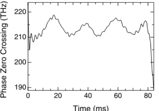
Figure 9 shows the retrieved pulse timing, corresponding to the temporal derivative of the linear fit to the spectral phase. Figure 10 shows the extrapolated zero crossing point of the spectral phase as a function of time. This point is quite sta-bly located near 215 THz, i.e., close to the center of the optical spectrum at 224 THz. (The large excursions at the start and the end of the trace are caused by the sliding intersection of the fit and the frequency axis when the slope of the spectral phase

FIGURE 9 Pulse timing fluctuations retrieved from the phase of the optical modes (see text)

FIGURE 10 Zero crossing point of a linear fit to the spectral phase as a func-tion time

FIGURE 11 Power spectral density of the pulse timing jitter

is close to zero.) This result excludes mechanical instabilities of the cavity as source of the slow timing drift because these would cause a linear phase passing the origin of the frequency axis. The 50-Hz noise modulatesνrot, indicating that the cen-ter of rotation associated with 50-Hz noise alone is located somewhere else. We also observe that optical phase fluctua-tions which remain after subtracting the contribution of timing jitter are on the order of a few milliradians only, showing that timing jitter is the main source of optical phase noise. The power spectrum of the timing jitter is plotted in Fig. 11. Com-pared with the quantum noise limit for timing jitter [13, 14], the measured noise is up to 30 dB higher at 50 Hz. Towards higher frequencies, where the influence of technical noise sources is weaker, the timing jitter approaches the quantum noise limit. Above≈ 20 kHz the power density reaches the measurement noise floor. We measure an rms pulse timing de-viation between the two lasers of 270 fs, when integrating over the spectral range from 100 Hz–100 kHz. Note that the sig-nificantly larger rms value of multiple picoseconds in Fig. 9 mostly results from noise at frequencies below 100 Hz. 6 Conclusions and outlook

In conclusion, we have demonstrated a method to measure the relative optical phase fluctuations of two lasers. The technique allows one to measure not only the average phase but simultaneously the phase fluctuations of each opti-cal line in the spectrum of the lasers separately. In this way, we obtain not only the phase noise of each mode, but also the noise on other quantities, for example pulse timing or pulse chirp. In principle, relative fluctuations of every aspect of the pulse trains are accessible from the measured data. The

method is especially suited for the characterization of pulse trains with a high duty cycle (long pulse compared to pulse distance) which is typically fulfilled for lasers with high rep-etition rates in the multi-GHz regime.

We have experimentally demonstrated the method by measuring the relative phase noise of two passively mode-locked 1.3-µm Nd:YVO4 lasers operating at a repetition rate of 5 GHz. We also obtain information on the intensity noise of the optical modes. From the simultaneously meas-ured optical phases, we have extracted the timing jitter of the lasers and found that it is the main cause of phase noise. At the same time, we could exclude mechanical instabilities as the source of timing drifts. This result we could not have obtained with a conventional method for timing jitter meas-urements [3, 4, 6, 15]. As a byproduct of the evaluation, we confirmed that the spacing of the optical modes in the spectra of the lasers is equidistant to better than 4 Hz rms over a span of optical frequencies of 140 GHz.

We believe that the presented method is an excellent tool for the identification of noise sources and noise coupling mechanisms in mode-locked lasers. A simple approach to do this would be to modulate a certain parameter (pump power, cavity length, etc.) and monitor its effect on the optical phase noise (and timing jitter, pulse chirp, etc.). This is interesting from a scientific point of view, because we can gain insight into the physics taking place inside a laser cavity. On the other hand, this knowledge may be used to eliminate noise-generating mechanisms and ultimately to the construction of lasers with lower noise.

ACKNOWLEDGEMENTSWe acknowledge the invaluable sup-port by S. Pawlik and B. Schmidt from Bookham Z ¨urich who contributed commercially unavailable but crucial pump diodes for the lasers used in the experiments. This work was supported in part by the European Commis-sion through the CRAFT project MULTIWAVE (018074) and the Hasler Foundation in Switzerland.

REFERENCES

1 H.R. Telle, G. Steinmeyer, A.E. Dunlop, J. Stenger, D.H. Sutter, U. Keller, Appl. Phys. B 69, 327 (1999)

2 R. Paschotta, A. Schlatter, S.C. Zeller, H.R. Telle, U. Keller, Appl. Phys. B 82, 265 (2006)

3 D. v.d. Linde, Appl. Phys. B 39, 201 (1986)

4 M.J.W. Rodwell, D.M. Bloom, K.J. Weingarten, IEEE J. Quantum Elec-tron. QE-25, 817 (1989)

5 R.K. Shelton, S.M. Foreman, L.-S. Ma, J.L. Hall, H.C. Kapteyn, M.M. Murnane, M. Notcutt, J. Ye, Opt. Lett. 27, 312 (2002)

6 R. Paschotta, B. Rudin, A. Schlatter, G.J. Spühler, L. Krainer, N. Haverkamp, H.R. Telle, U. Keller, Appl. Phys. B 80, 185 (2005) 7 T. Okoshi, K. Kikuchi, A. Nakayama, Electron. Lett. 16, 630 (1980) 8 H. Ludvigsen, M. Tossavainen, M. Kaivola, Opt. Commun. 155, 180

(1998)

9 E. Benkler, N. Haverkamp, H.R. Telle, R. Paschotta, B. Rudin, A. Schlat-ter, S.C. Zeller, G.J. Spühler, L. Krainer, U. Keller, presented at Confer-ence on Lasers and Electro-Optics (Baltimore, 2005)

10 K. Haneda, M. Yoshida, M. Nakazawa, H. Yokoyama, Y. Ogawa, Opt. Lett. 30, 1000 (2005)

11 H.R. Telle, B. Lipphardt, J. Stenger, Appl. Phys. B 74, 1 (2002) 12 H.K. Tsang, R.V. Penty, I.H. White, R.S. Grant, W. Sibbett, J.D. Soole,

H.P. LeBlanc, N.C. Andreadakis, R. Bhat, M.A. Koza, J. Appl. Phys. 70, 3992 (1991)

13 H.A. Haus, A. Mecozzi, IEEE J. Quantum Electron. QE-29, 983 (1993) 14 R. Paschotta, Appl. Phys. B 79, 163 (2004)

15 T.R. Schibli, J. Kim, O. Kuzucu, J.T. Gopinath, S.N. Tandon, G.S. Pet-rich, L.A. Kolodziejski, J.G. Fujimoto, E.P. Ippen, F.X. Kärtner, Opt. Lett. 28, 947 (2003)