Calibration graphs in isotope dilution mass spectrometry

(1)

Publisher’s version / Version de l'éditeur:

Analytica Chimica Acta, 896, pp. 63-67, 2015-10-08

READ THESE TERMS AND CONDITIONS CAREFULLY BEFORE USING THIS WEBSITE.

https://nrc-publications.canada.ca/eng/copyright

Vous avez des questions? Nous pouvons vous aider. Pour communiquer directement avec un auteur, consultez la

première page de la revue dans laquelle son article a été publié afin de trouver ses coordonnées. Si vous n’arrivez pas à les repérer, communiquez avec nous à PublicationsArchive-ArchivesPublications@nrc-cnrc.gc.ca.

Questions? Contact the NRC Publications Archive team at

PublicationsArchive-ArchivesPublications@nrc-cnrc.gc.ca. If you wish to email the authors directly, please see the first page of the publication for their contact information.

NRC Publications Archive

Archives des publications du CNRC

This publication could be one of several versions: author’s original, accepted manuscript or the publisher’s version. / La version de cette publication peut être l’une des suivantes : la version prépublication de l’auteur, la version acceptée du manuscrit ou la version de l’éditeur.

For the publisher’s version, please access the DOI link below./ Pour consulter la version de l’éditeur, utilisez le lien DOI ci-dessous.

https://doi.org/10.1016/j.aca.2015.09.020

Access and use of this website and the material on it are subject to the Terms and Conditions set forth at

Calibration graphs in isotope dilution mass spectrometry

Pagliano, Enea; Mester, Zoltán; Meija, Juris

https://publications-cnrc.canada.ca/fra/droits

L’accès à ce site Web et l’utilisation de son contenu sont assujettis aux conditions présentées dans le site LISEZ CES CONDITIONS ATTENTIVEMENT AVANT D’UTILISER CE SITE WEB.

NRC Publications Record / Notice d'Archives des publications de CNRC:

https://nrc-publications.canada.ca/eng/view/object/?id=c963874f-036a-4da0-9def-eead416e46d9

https://publications-cnrc.canada.ca/fra/voir/objet/?id=c963874f-036a-4da0-9def-eead416e46d9

(2)

Calibration graphs in isotope dilution mass

spectrometry

Enea Pagliano, Zoltan Mester and Juris Meija

Measurement Science and Standards, National Research Council Canada, 1200 Montreal Road, Ottawa ON K1A 0R6, Canada

E-mail: juris.meija@nrc-cnrc.gc.ca

Abstract. Isotope-based quantitation is routinely employed in chemical measurements. Whereas most analysts seek for methods with linear theoretical response functions, a unique feature that distinguishes isotope dilution from many other analytical methods is the inherent possibility for a nonlinear theoretical response curve. Most implementations of isotope dilution calibration today either eliminate the nonlinearity by employing internal standards with markedly different molecular weight or they employ empirical polynomial fits. Here we show that the exact curvature of any isotope dilution curve can be obtained from three-parameter rational function, y = f (q) = (a0 + a1q)/(1 + a2q), known as the

Pad´e[1,1] approximant. The use of this function allows eliminating an unnecessary source of error in isotope dilution analysis when faced with nonlinear calibration curves. In addition, fitting with Pad´e model can be done using linear least squares.

Keywords: isotope dilution, stable isotope labeled internal standards, calibration graphs, nonlinearity

Publication record

Analytica Chimica Acta (2015) 896, 63-67. doi: 10.1016/j.aca.2015.09.020

Copyright c

(3)

Calibration graphs in IDMS 2 1. Introduction

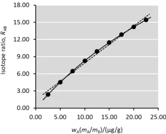
In isotope dilution, a sample is mixed with isotopic internal standard and the isotope amount ratio of the resulting blend is measured. In biomedical sciences this method is often known as the calibration with isotope-labeled internal standard normalization. Frequently, in order to calculate the amount of the analyte in the sample, a graphical approach is employed whereby the resulting isotope ratios are plotted against the mixtures of the isotopic standard with known amounts of natural standard (Figure 1). In situations when the resulting curve is not sufficiently linear due to the significant spectral overlap between the analyte and isotopic standard [1], polynomial empirical functions have been proposed to approximate the curvature of the isotope dilution function.

The adversity to nonlinear calibration plots has led to a variety of arbitrary calibration practices in isotope dilution. Perhaps true a decade ago, performing a nonlinear fitting is no longer an arduous task in the era of abundant supply of software. Despite this, many linearization methods have been proposed. Most notably, in 1981 Bush and Trager proposed plotting nB/(nA+ znB) against RAB instead of the traditional approach where RAB is plotted against amount ratios of the analyte (A) and isotopic internal standard (B), nA/nB [2]. In this linearization procedure the auxiliary parameter z is the denominator-isotope abundance ratio of the spike and the analyte, z = xref,B/xref,A, and therein lies a key assumption of the Bush-Trager approach: linear least squares fitting is possible only when the exact value of z is known. In practice, however, the value of z is often unknown and needs to be measured. Likewise, Colby and McCaman proposed to plot [(RB − RAB)/(RAB− RA)] × [(1 + RA)/(1 + RB)] against nA/nB (for two-isotope systems) [3]. A common feature to such linearization methods is to incorporate the isotopic composition of the analyte and the spike into the dependent variable of the regression but the uncertainty of the obtained fitting parameters that is due to these correction factors (z, RA, RB) remains ignored.

Other attempts have been taken to avoid the nonlinear calibration graphs in isotope-based quantitation: omission of the nonlinear portion of data, use of inverse ratios [4], use of statistical weighing schemes to counter the effects of nonlinearity [4], or logarithmic coordinate transformations [5]. As early as in 1983, a suggestion was made that “the eventual curvature of IDMS calibration curves can be described very accurately by means of higher order polynomials”[6]. Indeed, the use of quadratic [7] or cubic [8] polynomials remains popular to this day [9, 10]. In mixtures of the analyte and its

Figure 1. Nonlinear response in isotope dilution. The application of isotope dilution in life sciences commonly employs a calibration curve whereby the isotope ratios of the analyte and isotopic internal standard peak areas are plotted against their mass ratios. Here, the analyte (A) is cholesterol, the internal isotopic standard (B) is [13_C

3]-cholesterol (containing three 99

%-enriched carbon-13 atoms), and the isotope ratio represents the ratio of the major isotope signals from A and B. Numerical details of this plot are given in the Supporting Information.

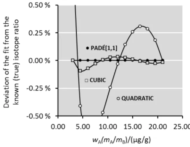
isotopically labeled internal standard, the general functional relationship between the isotope ratio and the mass ratio of these two substances is neither linear nor polynomial. Rather, it is a ratio of two linear functions. In fact, if the curve shown in Figure 1 were to be described (fitted) with a quadratic polynomial, one obtains a half-percent average deviation from the true curvature as shown in Figure 2. Albeit half-percent may indeed be an acceptable error to many, analysts should be aware that there are better functions available for isotope-based calibration when dealing with nonlinear calibration plots. This note brings attention to the fact that the use of polynomial curves in isotope dilution introduces unnecessary errors which can be avoided by using rational Pad´e[1,1] equation and linear least squares fitting.

2. Theory 2.1. The equation

The use of rational functions to describe the isotope dilution curves becomes evident from the rearrangement of the isotope dilution equation. In particular, the isotope dilution equation [11]

wA= wBRB− RAB RAB− RA mB(AB) mA(AB) MAP RA MBP RB (1)

(4)

Figure 2.Higher order polynomials do not describe the isotope dilution curves “very accurately”as it is commonly believed. Here, the theoretical isotope ratios from Figure 1 are fitted with quadratic and cubic polynomials, and the deviations of the fitted results from the true values are shown here. Pad´e[1,1] fit is also given for comparison. Numerical details of this plot are given in the Supporting Information.

inverts with respect to RAB into a first-order Pad´e function, RAB-i = (a0+ a1qi)/(1 + a2qi), where qi = wAmA(AB)-i/mB(AB)-i: RAB-i= a0+ a1(wAmA(AB)-i/mB(AB)-i) 1 + a2(wAmA(AB)-i/mB(AB)-i) (2) where a0= RB (3) a1= RAa2 (4) a2= w−1 B MBP RB MAP RA (5)

The notation used in the above equations is explained in Table 1. In addition, Eq. (2) will also be denoted as y = f (q) = (a0+ a1q)/(1 + a2q) where y and q represent dependent and independent regression variables, respectively. Hence, the general isotope dilution curve is described using the Padé[1,1] function (Eq. (2)) with three fitting parameters. It is important to reiterate that, unlike the polynomial equations which are empirical approximations of the isotope dilution curve, Padé[1,1] function provides an exact description of the curve. Consequently, the use of Padé equation for isotope dilution will not incur additional errors due to the arbitrary choice of the model equation. In addition, one does not have to resort to a larger number of fitting parameters in order to describe more pronounced curvatures as it is practiced with polynomials. Last, but not least, Padé[1,1] is a monotonous function and does not have inflection points in contrast to polynomials. All of

these properties make Pad´e[1,1] reliable not only for interpolation but also for extrapolation which is useful in the method of standard addition [12].

2.2. The fitting

It has been long known that the curvature of isotope dilution curves is described by rational function [13], and early isolated attempts to employ this function using non-linear fitting procedures appear as early as in 1977 [14]. The non-linear fitting of the rational functions in isotope dilution, however, has not found widespread acceptance likely due to its complexity. In this vein, we draw attention to the fact that, similar to linear and polynomial models, fitting with Pad´e[1,1] equation, y = (a0+ a1q)/(1 + a2q), can also be performed using the linear least squares method whereby the fitting parameters (a0, a1, a2) are given by the familiar matrix expression [15].

a= (QTQ)−1_QT_Y ₍₆₎ Here Q is the regression design matrix and Y is the vector of predictor values (typically, the measured isotope ratios). Design matrix Q in Eq. (6) is N × k matrix containing the input variables where N is the number of measurements and k is the number of fitting parameters. For the Pad´e[1,1] model, one can use

Q= {1, q, −qy} (7) which follows from the rearrangement of y = (a0+ a1q)/(1 + a2q) into y = a0 + a1q − a2qy. Fitting parameters can be obtained using the Microsoft Excel’s LINEST function [12] and one can also obtain explicit solution of Eq. (6): a=   N P q −P qy P q P q2 ₋_{P q}2_y P qy P q2_y ₋_{P q}2_y2   −1  P y P qy P qy2   (8) The linear least squares fitting with Padé[1,1] [16, 17] involves both dependent and independent variables (y and q) and, strictly speaking, it does not satisfy the least squares condition for a minimum value of P [yi− f (qi)]2_. _{However, despite the fact that the} above least squares approach for Padé[1,1] does not yield the lowest residual regression variance possible, it nevertheless outperforms polynomial functions (see Figure 2). Consequently, the approximate nature of linear fitting with Padé[1,1] does not impede its usefulness. Needless to say, rigorous nonlinear fitting algorithms are readily available if necessary.

2.3. Calculation of the result

When polynomial expressions are employed in the standard fashion whereby the y-axis is established

(5)

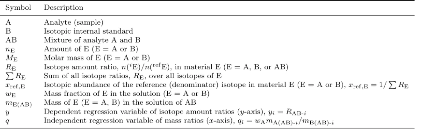
Calibration graphs in IDMS 4 Table 1. Standard symbols employed in this work.

Symbol Description A Analyte (sample) B Isotopic internal standard AB Mixture of analyte A and B nE Amount of E (E = A or B)

ME Molar mass of E (E = A or B)

RE Isotope amount ratio, n(iE)/n(refE), in material E (E = A, B, or AB)

P

RE Sum of all isotope ratios, RE, over all isotopes of E

xref,E Isotopic abundance of the reference (denominator) isotope in material E (E = A or B), xref,E= 1/PRE

wE Mass fraction of E in the solution (E = A or B)

mE(AB) Mass of E (E = A, B) in the solution of AB

y Dependent regression variable of isotope amount ratios (y-axis), yi= RAB-i

q Independent regression variable of mass ratios (x-axis), qi= wAmA(AB)-i/mB(AB)-i

from the measured isotope ratios and the x-axis is formed from the mass of the analyte in the standard solutions (normalized to the mass of the internal standard), one needs to perform polynomial inversion in order to obtain the mass of the analyte in the analyzed sample. This is an unnecessary complication (especially for the cubic polynomial). Coordinate swapping obviates the problem of polynomial inversion, but another complication arises polynomial functions do not give stable results with coordinate swapping of isotope dilution plots. Unlike polynomial expressions, however, Padé[1,1] function is readily invertible, a feature which arises from the fact that the inverse of Padé[1,1] function is also a Padé[1,1] function: y = (a0+a1q)/(1+a2q) inverts into q = (a0−y)/(a2y −a1). The complexity of this inversion is comparable to the linear regression where y = a0 + a1q leads to q = (y − a0)/a1.

3. Experimental

Mass fraction of bromide was determined in synthetic water samples using negative chemical ionization gas chromatography mass spectrometry after aqueous derivatization of bromide ions with triethyloxonium salt at ambient temperature. Analytical procedures, such as the sample aliquoting or the addition of isotopic internal standard, were performed gravimetrically. All 5 g aliquots of the calibration standards or samples (ranging in the mass fraction of bromide from 0.0 to 9.6 µg/g) were spiked with ca. 5 g of isotopic internal standard containing w(79_Br−_{) = 2.3 µg/g. Calibration} plots were obtained by plotting the observed isotope ratio of81Br to79Br versus the variable wA(mA/mA) where wAis the mass fraction of bromide in the natural standard, mA is the mass of the natural standard aliquot, and mB is the mass of the isotopic internal standard (bromine-79 labeled bromide) added to the sample aliquot. More detailed account of this method are not pertinent to this manuscript and these can be

consulted elsewhere, if necessary [11, 18]. Supporting Information provides all measurement results employed in this manuscript.

4. Discussion

When sufficient linearity of the calibration curve cannot be achieved, analysts may resort to nonlinear fitting. In isotope-based quantitation, however, one does not have to use empirical polynomial functions because the true nonlinear model is given by the Pad´e[1,1] equation. The Pad´e[1,1] equation involves three parameters. Hence, an isotope dilution calibration can be performed with the minimum of three standard/spike mixtures, and measurement of the sample requires the subsequent fourth mixture that of the sample and the isotopic spike. This procedure is called the quadruple isotope dilution. One can also employ less exhaustive isotope dilution strategies whereby some of the coefficients in Eq. (3) are established from other sources. For example, if all variables in Eq. (3) are given, one can establish the calibration plot (Eq. (2)) without any recourse to experiment. Albeit rarely used, this corresponds to the single isotope dilution. A common single-point calibration strategy establishes the calibration plot by analyzing a single calibration blend in order to obtain wB (double isotope dilution).

The performance of Pad´e[1,1] model (Eq. (2)) can also be demonstrated with experimental data. For this purpose, determination of bromide was performed in synthetic samples with known levels of bromide. Five-level calibration curve with 0.00, 0.51, 1.02, 1.60 and 2.08 µg/g of bromide was constructed with all isotope ratio measurements done in triplicate, and the obtained curve was fitted with linear, quadratic, cubic and Pad´e[1,1] functions as per Eqs. (6) and (7) (Figure 2). Four samples with known levels of bromide (0.10, 0.70, 1.31, and 1.73 µg/g) were then analyzed in triplicate and the results were obtained by using

(6)

Table 2. Errors (biases) due to the choice of model equation as exemplified in the determination of bromide using isotope dilution GCMS methoda_. Calibration molde Sample 1 wBr= 0.10 µg/g Sample 2 wBr= 0.70 µg/g Sample 3 wBr= 1.31 µg/g Sample 4 wBr= 1.73 µg/g Average absolute bias Linear –66.1 % +14.7 % +6.3 % +0.5 % 21.9 % Quadratic +3.2 % +1.8 % –1.4 % –0.8 % 1.8 % Cubic +2.5 % +0.8 % –0.7 % 0.0 % 1.0 % Pad´e[1,1] +1.4 % +0.6 % –0.5 % +0.1 % 0.6 %

a_{Consult the Supporting Information for detailed results and calculations.}

linear, quadratic, cubic and Pad´e[1,1] models for the calibration plot (see Table 2).

From the results presented in Figure 2 and Table 2, it is clear that quadratic model can give significant errors in isotope-based quantitation. Although the cubic model provides reasonable performance, its use should be discouraged for several reasons; it is empirical model of high mathematical complexity and requires more fitting parameters than necessary. In this regard, Pad´e[1,1] model satisfies all the theoretical and practical requirements which polynomial models fail to do. Additional advantage of applying the Pad´e[1,1] model over the existing linearization approaches (Bush-Trager or Colby-McCaman) is that isotopic composition of pure components (RA, RB) is no longer required in order to construct the calibration plot. In particular, this means that one does not have to perform assay of pure isotopic internal standard.

An important consequence of the fact that Pad´e[1,1] model is not an empirical choice is its predictive power. To illustrate this, two additional samples were measured for which the isotope ratios fall well outside the calibration interval: sample 5 (wBr = 2.77 µg/g) and sample 6 (wBr = 9.63 µg/g). The results are shown in Figure 3. Although it is not a common practice in analytical chemistry to extrapolate calibration curves, the predictive power of Pad´e[1,1] offers the ability to obtain results with reasonable accuracy when extrapolation is performed in isotope-based quantitation. One can clearly not say the same when empirical polynomial models are used.

5. Conclusion

There are two reasons why non-linear calibration plots are usually avoided: it is not trivial to postulate an appropriate model from physical point-of-view and the fitting parameters usually have to be estimated iteratively. Both of these shortcomings are addressed in isotope-based quantitation with the use of three-parameter Pad´e[1,1] function. Fitting with both Pad´e[1,1] and quadratic polynomial require a minimum of three data points, and both curves can be obtained using almost identical least square design

Figure 3. The predictive power of the various regression models in isotope-based quantitation. The five black points with bromide levels from 0.00 to 2.08 µg/g are used to construct the calibration curve using linear, quadratic, cubic, and Pad´e[1,1] models (same as in Table 2) whereas the two white points at 2.77 and 9.63 µg/g show the measured isotope ratios in two additional samples which fall well outside the calibration range. The superior predictive power of the Pad´e[1,1] model shows the advantages of selecting a model based on first principles. Numerical details of this plot are given in the Supporting Information.

matrices. Unlike the Pad´e[1,1] function, however, the quadratic function is an arbitrary model which can give additional errors. In this vein, it is hoped that mass spectrometers will soon enable fitting with Pad´e[1,1] instead of the polynomial functions in their software. Appendix

Supplementary data related to this article can be found at http://dx.doi.org/10.1016/j.aca.2015.09.020. References

[1] Tan A, Lévesque I A, Lévesque I M, Viel F, Boudreau N and Lévesque A 2011 Journal of Chromatography B 8791954–1960 URL http://dx.doi.org/10.1016/j. jchromb.2011.05.027

(7)

Spec-Calibration graphs in IDMS 6 trom. 8211–218 URL http://dx.doi.org/10.1002/bms.

1200080505

[3] Colby B N and McCaman M W 1979 Biol. Mass Spectrom. 6225–230 URL http://dx.doi.org/10.1002/ bms.1200060602

[4] Schoeller D A 1976 Biol. Mass Spectrom. 3 265–271 URL http://dx.doi.org/10.1002/bms.1200030603

[5] Klein P D, Haumann J R and Eisler W J 1972 Analytical Chemistry 44 490–493 URL http://dx.doi.org/10. 1021/ac60311a020

[6] Jonckheere J A, Leenheer A P D and Steyaert H L 1983 Analytical Chemistry 55153–155 URL http://dx.doi. org/10.1021/ac00252a042

[7] Duncan M W, Gale P J and yergey A L 2006 The principles of quantitative mass spectrometry (Denver, Colo: Rockpool Productions) ISBN 978-0978605803 [8] Olson E S, Diehl J W and Froehlich M L 1988 Analytical

Chemistry 60 1920–1924 URL http://dx.doi.org/10. 1021/ac00169a016

[9] Alonso J I G and Rodriguez-Gonzalez P 2013 Isotope dilution mass spectrometry (Cambridge: Royal Society of Chemistry) ISBN 1849733333

[10] 8000B M Determinative chromatographic separations [11] Pagliano E, Mester Z and Meija J 2013 Anal Bioanal

Chem 405 2879–2887 URL http://dx.doi.org/10. 1007/s00216-013-6724-5

[12] Meija J, Pagliano E and Mester Z 2014 Analytical Chemistry 86 8563–8567 URL http://dx.doi.org/10. 1021/ac5014749

[13] Pickup J F and McPherson K 1976 Analytical Chem-istry 48 1885–1890 URL http://dx.doi.org/10.1021/ ac50007a019

[14] Min B and Garland W 1977 Journal of Chromatography A 139 121–133 URL http://dx.doi.org/10.1016/ S0021-9673(01)84132-7

[15] Taavitsainen V M 2013 Chemometrics and Intelligent Laboratory Systems 120136–141 URL http://dx.doi. org/10.1016/j.chemolab.2012.11.001

[16] Ratkowsky D A 1987 Can. J. Chem. Eng. 65 845–851 URL http://dx.doi.org/10.1002/cjce.5450650519

[17] Bartkovjak J and Karovicova M 2001 Measurement Science Review 1 63–65 URL www.measurement.sk/PAPERS/ Bartkov.pdf

[18] Pagliano E, Meija J, Sturgeon R E, Mester Z and D’Ulivo A 2012 Analytical Chemistry 84 2592–2596 URL http: //dx.doi.org/10.1021/ac2030128