An analysis of nine-ending pricing

An Analysis of Nine-ending Pricing

Wei Wu

B.A., Tsinghua University (1997) M.A., Simon Fraser University (1999) Submitted to the Sloan School of Management in partial fulfillment of the requirements for the degree of

Master of Science

at the

MASSACHUSETTS INSTITUTE OF TECHNOLOGY June 2004

®

The author hereby grants to Massachusetts Institute of Technology permission to reproduce and distribute publicly paper and electronic copies of this thesis document in whole or in part, and to grant others

the right to do so.

Signature of Author ...

...

Sloan School of Management

28 2004

Certified by .

...

...

...

John D.C. Little

Institute Professor

Accepted

by ...

MASSACHUSETTS INST 'lE

OF TECHNOLOGY DEC 0 6 2004 LIBRARIES I i i

An Analysis of Nine-ending Pricing

by

Wei Wu

Submitted to the Sloan School of Management on 28 May 2004, in partial fulfillment of the

requirements for the degree of Master of Management Science

Abstract

Prices ending in 9 are ubiquitous. In this paper I first develop a theoretical model of the effect of such prices on sales and review the empirical literature on the topic. Then I use a data set from an online experiment run by Lau (2000) to conduct an empirical study of the effect. Analysis with a logit model indicates that products with 9-ending prices are more likely to be chosen than others but a high fraction of 9-endings decreases the effect.

Thesis Supervisor: John D.C. Little Title: Institute Professor

Acknowlegements

I greatly appreciate Professor John D.C. Little for his guidance, encouragement and enormous help throughout my study at MIT. I learned from him how to conduct serious research and think critically, and most importantly, the necessary character to be a real scholar. It is a privilege for me to have the opportunity to work with and learn from him, an outstanding academic leader and great mentor, as well as a master of humor.

I thank Professor Dan Ariely, for his encouragement and suggestions for my aca-demic career and Professors Duncan Simester and Jin Gyo Kim for their help during my study period at MIT. I also appreciate the teaching and interaction of Professors Shane Frederick, John Hauser, Drazen Prelec, Glen Urban and Birger Wernerfelt.

I thank my colleague students at MIT, On Amir, Leonard Lee, Kristina Sham-pan'er, Jiwoong Shin, Peng Sun, Olivier Toubia, Ray Weaver and Rober Zeithammer.

I want express my thanks to my classmates and friends who gave me encourage-ment, help and shared the happiness with me: David Li, Li He, Mahesh Kumar, Wei Peng, Ludan Liu and Jenny Vickers.

The secretaries in the MIT Marketing Group, Rosa Blackwood and Sandra Crawford-Jenkins offered me a lot of help, which I appreciate very much.

Finally, I would like to thank my wife, Kun Zhang, who gave up her starting career of lawyer in China and joined me, for her support and companion, my daughter Elaine, who brings us great joy, and my parents, who always support me unconditionally.

Contents

1 Introduction 7

2 Literature Review 10

2.1 Empirical Evidence for the Existence of Price-Ending Meanings . . . 15 2.2 Empirical Analysis of Price Endings with Scanner Data ... 17 2.3 The Change of 9-ending Effect due to the Fraction of 9-endings . . . 18

3 A Theoretical Model of 9-ending 19

4 The Design of Lau's Experiment

28

5 Empirical Analysis 31

5.1 Dependent and Explanatory Variables . . . ... 32

5.2 Modelling 9-ending Effects on Purchase Decisions ... 33 5.2.1 Interaction between 9-endings and 9-counts in the within

cate-gory effect . . . ... . 34 5.2.2 Purchase Stimulation Effect . . . ... 34

5.3 Functional Form ... 35

6.1 Estimates of coefficients not related with 9-endings ... 40 6.2 Estimates for 9-ending effects ... 41

7 Extension and Discussion

43

7.1 Linear 9-ending within-category effect ... 43 7.2 Effect of budget on the effectiveness of 9-endings ... 45

8 Conclusion 51

Chapter

1

Introduction

Prices with nine-endings are almost everywhere, from grocery stores to electronics shops, from new products to items on sale. The popularity of nine-endings raises an interesting research question: what are their effects on customer purchasing behavior, including whether or not to purchase from a category, which brand to choose and the purchase quantities. The prices that end in nine have attracted many researchers' attention because of their popularity with retailers.

Previous studies found that nine-endings have a positive effect on customers' choice. (For example, Schindler and Kibarian, 1996 [14] showed evidence of this effect.) However, recent studies suggested that a high fraction of nine-ending prices will decrease the positive effects of nine-endings. (See Ouyang, 1998 [11]; Anderson

and Simester, 2003 [1]; Lau, 2000 [6]).

In this paper, we will continue the line of research that examines these two effects. Nine-endings can possibly make people perceive a lower price by taking cents off from the price. For example, an item of price $2.99 might seem much cheaper than an item with price $3.02 although the latter one costs only 3 cents more. Nine-endings may also signal a "bargain", which will increase customers' likelihood to purchase.

On the other hand, a saturation of nine-endings might lower their positive effects on customers' purchases. The reason is that nine-endings on various items in differ-ent categories compete for the limited dollars in customers' pockets. Consequdiffer-ently, positive and negative effects are interwoven.

In this paper, we exploit data from an on-line grocery purchase experiment de-signed to study nine-ending effects. The experiment is well controlled and gives us a very clean data set about people's purchase behavior. Not surprisingly, a poten-tial criticism of the data is that the experiment is different from the real purchase environment. However, as we describe in a later section, the experiment was thought-fully designed to mimic key features of real shopping. For example, the categories, items, prices are all real and people doing the experiment have the right motivation to purchase as if they were doing their weekly shopping in a grocery store. There-fore, we believe that the nine-ending effects are neither appreciably weakened nor

strengthened with respect to the variables being manipulated.

The rest of the paper is organized as follows. Section 2 reviews empirical literature about nine-endings. Section 3 develops a theoretic model of price-endings. Then Section 4 described briefly the experimental design and the data. Section 5 and 6 show the estimation results. Section 7 continues with some extension and discussion. Section 8 concludes.

Chapter 2

Literature Review

Researchers have documented a great amount of evidence that the digit 9 occurs among the rightmost digits of retail prices far more than chance would predict. It has been suggested by some scholars (e.g. McCarthy and Perreault 1993, p.547, [8]) that the overrepresentation of 9 digits in retail price endings is merely the persistence of a retailing practice that originated in attempts by early retailers to lessen dishonesty of clerks. Nine-ending prices make them use the cash register to make change to customers and thus prevent them from pocketing the payments. However, electronic devices are now widely used in almost all retail stores and yet 9 endings are still used everywhere. Researchers propose different explanations. The one with the most intuitive appeal is underestimation of actual prices, that is, a tendency of consumers

to perceive a 9-ending price as a round-number price by cutting the rightmost digit to 0.

Schindler and Kirby (1997, [15]) applied the concept of cognitive "accessibility" to describe consumers' psychological process to price endings.' Simple and easy rep-resentation tends to be much more accessible than complicated (though complete) representation. In the price endings context, prices with round number endings are easy to remember and processed by consumers. Because consumers favor the use of round numbers in their cognitive processing of price information, they may translate a price into a round-numbered mental representation. Two strategies could be used for this encoding: rounding and truncation. Rounding starts with attending sequen-tially to each digit of the price. Then the customer uses a rounding rule to arrive at a round number provided the original ending is not a round number. A commonly used rounding rule is to round down to the next lower O-ending if the original ending is less than 4, or to round up to the next higher O-ending if the rightmost number is greater than 5. Truncation means simply cut the rightmost digit to 0 to achieve a round number. Clearly, truncation requires much less mental effort than rounding: fewer digits need to be processed and no complex rounding rule needs to be imple-mented. Schindler and Wiman (1989 [16]) also found empirical evidence supporting

1

Accessibility is often termed as "availability" (Tversky and Kahneman, 1973 [22]), which is characterized as easy to be used in thought.

the idea that customers use the truncation strategy. The underestimation effect that truncation generates, therefore, benefits retailers using 9-endings. They also surveyed the real price-endings and found that the most popular price endings are 9 (30.7%), 0 (27.2%) and 5 (18.5%). More than 3 quarters of price endings consist of these three digits. The overrepresentation of 0 and 5 can be accounted by the high cognitive accessibility of 0- and 5-endings. The overrepresentation of 9-endings can be partly explained by the underestimation effect.

There is also a general awareness in marketing research that price can serve as informational cues other than the cost of purchase. Shindler (1991 [17]) discussed the symbolic meanings of price endings. For example, the endings of $39.99 may connote a discount (or consumers interpret it as a discount). The rounding endings like $300 might connote high quality and an "odd" ending like $10.47 might connote a carefully determined price. Because the price endings can be manipulated without substantial changes of the price levels, they can possibly be used strategically. Schindler argued that the symbolic meaning of a price ending can be distinguished from the effects due to consumers' perception of the price levels (i.e., underestimation effect). In other words, $39.88, $39.95, $39.99 are basically all prices just below $40 and should be perceived by consumers as the same price level; but their different endings can convey or create different information or impression to customers.

Schindler (1991 [17]) argued that the symbolic meaning can be distinguished from the perception effect. Suppose there are two segments of customers: Segment one simply does a truncation for price endings and the other segment carefully examines each digit of prices (e.g. the two segments of customers in my model to be presented in the next section). Then an item with price $39.99 would not have an underestimation effect for customers in the second segment but the connotation of "sales price" might still come to their minds.

Schindler (1991 [17]) also compiled possible meanings connoted by price-endings. For example, 9-endings might mean that the price is low, the price has been reduced, the price has not been increased recently or it is on sale. A natural question people raise is why a 9-ending is interpreted by customers as low price? Why other

end-ings, like 8, are not interpreted by customers as low prices? Schindler also gave his

explanation (Schindler, 1991 [17], P.799).

Retailers' beliefs (whether true or not) that consumers will underestimate the levels of just-below prices2 _{caused them to choose these endings in}

situations where a low price or a discount was an important selling point. In this sense, the possibility that consumers may underestimate just-below prices can be said to be a cause of just-below price endings connoting low or discount prices. And this interrelation would explain why both meaning and underestimation explanations of hypothesized price-ending effects often predict similar effects.

In recent years people did some interesting studies on non-nine price endings. Simmons and Schindler (2003 [19]) studied the impact of cultural superstitions and customs on the price endings used in Chinese advertising. The digit 8 in Chinese (pronounced as "bar") is similar in pronunciation to fa (pronounced as "far"), which means to get rich and to fu (pronounced as "foo") which means good fortune. Thus the digit 8 is associated with both prosperity and good luck, which are desirable for most people, especially people in commercial industry. On the other hand, digit 4 is pronounced exactly the same as "to die", except for the tone, and thus is associated with unhappy things. These meanings associated with digits influenced people's atti-tudes toward price-endings and consequently directs managers price setting. Because people love 8, it is very common to use a price like 3.88 instead of 3.99. Simmons and Schindler surveyed the market prices in China and found that the digit 8 is overrepre-sented with respect to chance among the rightmost salient ending digits of advertised prices and the digit 4 is underrepresented with respect to chance even among those rightmost salient ending digits that are not overrepresented.3 _{Their study showed}

that seemingly unrelated factors like superstitions can become the most important determinant for price-endings.

Stiving (2000 [20]) provided a theoretical explanation for why firms use round 3_{The distribution of rightmost salient ending digits in sampled prices is: 0, 9.2%; 1, 1.6%, 2,}

prices to signal quality. His model shows that firms that are using high prices to signal quality are more likely to set those prices at round numbers and low-quality

firms will use prices that end in 9. Recently, Shoemaker et al (2003 [18]) found that Stiving missed the constraint of non-negative demands. They also argued that by eliminating one of Stiving's assumptions, round prices are used much less often and 9-endings still prevail. Their comment on Stiving's work reveals opportunities for more robust explanations for quality signalling by round price endings.

2.1 Empirical Evidence for the Existence of

Price-Ending Meanings

One of the first detailed reports of empirical evidence that 9-endings can have mean-ings to customers is Schindler (1984 [13]). He studied whether price endmean-ings affect the ability of consumers to recognize whether a price has recently been increased and found that consumers are inclined to judge that the prices with just-below endings were ones which had not been increased. This study suggested that when memory failed to provide the needed information, the subjects responses were guided by an impression that prices with 9-endings are the ones which are less likely to have been recently increased.

Recently, Anderson and Simester (2003 [1]) conducted a field experiment which offered strong empirical support to the discount meaning of 9-endings. They worked with some catalog companies and designed the experiment by manipulating the price endings of their products. First they ran a small pilot study, in which four dresses were selected as "control condition", that is their prices are $39, $49, $59 and $79, respectively. They modified the price endings of these four items by adding and subtracting 5 dollars for each of them to create Test condition A and B (i.e., $34 and $44 for item 1, $44 and $54 for item 2, $54 and $64 for item 3 and $74 and $84 for item 4). A total of 66 dresses were sold in the $9 ending conditions, compared to 46 units in the $5 lower conditions and 45 units in the $5 higher conditions. Therefore, the 9-endings yielded a demand increase of approximately 40% for these four items, while the $10 price difference between the two Treatment conditions resulted in effectively no difference in demand. This study shows that the 9-endings indeed serve as "Sale" cues, at least when customers are not very familiar with the market prices of these

fashion products.

Anderson and Simester also did three other field studies in which price endings were experimentally manipulated. They found that the $9 price endings increased demand in all three studies. Furthermore, the new items have stronger increase of demand due to 9 endings than items which had been sold in previous years. They also found that the 9-endings were less effective when the catalog companies explicitly

use "Sale" cues. From these results they conclude that $9-endings are more effective when customers have limited information on the items they purchase.

Anderson and Simester's work show that 9-endings are effective cues for products unfamiliar to consumers. However, we can see that 9-endings are still commonplace for items people buy every week like groceries. Here we will conduct an empirical analysis based on groceries people buy in their daily lives.

2.2 Empirical Analysis of Price Endings with

Scan-ner Data

A big chunk of empirical studies of 9-endings use scanner data and logit model, which were pioneered by Guadagni and Little (1983, [4]). Little and Ginese (1987, [7]) used scanner data on pancake syrup and a logit model to study nine-ending effects. They included a variable for price and a dummy for each of the digits 0 through 8. Then 9-ending effects would be shown by negative and significant coefficients of each of the dummy variables. If this is true, then it supports the 9-ending does promote sales. They found that ending digit 9 is significantly preferred over the digits 0, 1, 2, 3, and 5 but not significantly different from endings with other digits.

the logit model to tuna and yogurt data. They found that the dummy variable for 9-ending was negative and significant for the tuna data and positive and insignificant for yogurt data. They offered some conjecture about the puzzling results but basically conclusions are difficult to draw.

2.3 The Change of 9-ending Effect due to the

Frac-tion of 9-endings

In recent years, more and more stores set almost all their prices with 9-endings. However, recent studies suggest that a high fraction of nine-ending-priced products reduces the positive effects of nine-endings (Ouyang, 1998 [11] and Anderson and Simester, 2003 [1]). In this paper, we will continue this line of research.

Chapter 3

A Theoretical Model of 9-ending

The ubiquity of price endings in 9 or 99 has been noticed and well documented. One explanation is that 9 endings convey the information that the firm contemplates carefully its prices and make every effort to set them as low as possible. However, it is not clear why 8- or 7-endings cannot serve the same purpose.

The explanation which has the most intuitive appeal is that consumers ignore the right digit(s) (i.e. $48.9 is processed as $48). Therefore the retailers can sell more without lowering prices too much. This cognitive explanation says that consumers are busy and the their brains have limited storage capacity; so they do not process the right digit(s) (Nagle, 1987, [10]). However, it is not very clear why consumers do not round the price by recalling $48.9 as $49.

Basu (1997 [2]) offered an economic equilibrium explanation for why there are so many 9 endings. In his paper, he chose to discuss 99-endings. The rationale is the same as 9-endings. Assume that there are thousands of goods in a retailer's store. Each product has a demand curve xi = xi((Di, Ci)), where (Di, Ci) represents the price of good i decomposed into Di dollars and Ci cents. Hence Di E N U {0} and

Ci E {0,1,...,99}.

Customers do not process Ci when they decide their purchases because of the high cognition and calculation costs of doing so. Instead they treat Ci as the expected value

EC, which they obtained by browsing and unwitting collection of information.

Given the consumers' strategy, the retailer's best strategy is to set Ci as 99 and price i as (i, 99) such that ri(bi, 99) > 7ri(Di, 99) for all non-negative inters Di.

Given the retailer's strategy, consumers' choice is also optimal because the expec-tation EC is not only the right one, but also identical to the real value. Therefore, the unique Nash equilibrium price profile that prevails in the market is given by

{(Di, 99)}i=1,2,....

Basu's model gives a Nash equilibrium explanation about why 99-endings are ubiquitous in the retailing market. His explanation receives support from some ex-perimental work by Ruffle and Shtudiner (2003 [12]). They offered an exex-perimental test for Basu's model and find ample support for it. They find that convergence to the

99-ending equilibrium is faster and more widespread when firms are able to observe the previous pricing decision of others.

Basu's model is unique in 9-ending literature because it offers a theoretical expla-nation of 99-endings in marketplace. Of course, Basu's story about why 99-endings are ubiquitous can be applied to 9-endings. However, the existence of non-9-endings (and non-99-endings) are non-neglectable (Schindler and Kirby, 1997, [15]). The co-existence of 9- and non-9-endings merits more research. What factors make retailers choose using non-9-endings? Which kinds of products should have 9-endings and which should not? Is there any optimal fraction of 9-endings? If yes, by which fac-tors is this optimal fraction determined? Recent empirical literature has documented evidence that overusing 9-ending will actually hurts demand (Ouyang, 1998 [11]; An-derson and Simester, 2003 [1] and Lau, 2000 [6]). I will study this issue in a theoretical model in this section.

The basic setup of my model is the following. A retailer sells many products to its customers. There are two segments of customers. Customers in segment 1 have high cognitive and calculation cost so they replace the last digit with the rational expectation of the price endings. Customers in segment 2 process the prices (including the last digits) as what they are. We can think the second segment consists of people who have more time or better calculation capacity. Alternatively, we can think of

this as two states of a typical consumer: with some probability s/he does not care the price-endings (when s/he is busy) and otherwise s/he really checks them.

The total number of customers is normalized to 1 and a fraction of IL belongs to Segment 1. For simplicity, we assume linear demand function: for a typical product

i, the demand is q(p) = c- kp, where q is the demand for that product, p is its price

and c, k are constants pertaining to that product. We draw a typical demand curves in Figure 3-1.

We decompose the price into the main price d, which is the price formed by replacing the ending by zero and dividing it by 10, and the price-ending, e. That is

p = 1Od + e. It is clear that the retailer's strategic space is So = N x {0, 1,..., 9).

Of course the retailer can set the price extremely high and nobody will buy but that is meaningless. Therefore, we only consider the strategy which makes the demand positive, that is, we only consider the strategic space such that d is bounded from the above. That is (d,e) E S - 0,

1,...,

A 0. ij) 110 ,PI N ~jp&,xN I 1. -01~CC el Bp%\N

The retailer's problem is,

max 7r(d,e) = ap. q(1Od + m) + (1 - )p q(1Od + e) (3.1)

s.t.

p = lOd+e,

q(x) = c- kx, for

Vx,

(d,e) E S.

where m is the expected price endings by consumers in Segment 1.

First let us look at two special cases first.

(i) I- = 1. That is, all customers are in Segment 1, then max r e = 9. We

replicated Basu's model.

(ii) = 0. That is, all customers are in Segment 2, then max 7r = e should be set as if it is just part of the price (i.e., no price ending effects).

(i) and (ii) are trivial. In addition to them, we know that if is very small (i.e. Segment 1 can be neglected), price endings should be set as if price ending effects do not exist. The interesting case is, how would the price endings be determined if is non-neglectable? We have the following proposition.

Proposition 1 As big enough, d*(k) is (weakly) decreasing in k and e*(k) is (weakly) increasing in k, where d*(k) and e*(k) are solution to problem (3.1) .

We defer the proof to the end of the chapter.

The above proposition says that, as price sensitivity (k) becomes large, the major part of the price (d) should be lowered (or at least not increased) and the price ending

(e) should be increased (or at least not decreased). Notice, however, that price endings have a ceiling of 9. Therefore, once the price ending reaches 9, it stays there as k is further increased.

The model offers a setting that encompasses several phenomena and permits trade-offs among them. If segment 2, with customers who see prices clearly without trunca-tion, is dominant ( is small), the retailer will maximize profit with prices that may take on any endings. As increases, segment 1 and truncation become dominant and so the retailer will switch to 9 endings.

Proposition 1 adds insight to this. For any y, increasing price sensitivity (k) leads to lower prices that eventually use all 9 endings.

However, any large retailer such as a grocery supermarket or a department store will have thousands of products and therefore will face a whole distribution of price sensitivities. This means that there will be conditions under which some products will have optimal prices that may end in any digit and a potentially large block of others, all of which end in 9. Thus the model comes up with insights that seem consistent with the pricing policies found in many supermarkets as well as rather different ones

in some department stores.

Because Problem (3.1) is an integer programming problem, it is almost hopeless to find closed form solution. Neither can we use implicit function theorem to prove because the discrete nature of the domain. To prove this proposition, we need the following extension of Topkis Theorem.

Theorem 2 (Monotonicity Theorem. Milgrom and Shannon 1994 [9]) Let f:

X x T -+ IR, where X is a lattice, T is a partially ordered set and Y C X. Then

arg maxEy f (x, t) is monotone nondecreasing in (t, Y) if and only if f is

quasisuper-modular in x and satisfies the single crossing property in (x; t).

We sketch the proof for Proposition 1.

Proof. Let's rewrite Problem (3.1) by substituting (2)-(4) into it and write 7r as a

function of (-d, e) instead of (d, e)

max

(-d,e)ES' r(-d, e; k) =

u[-10(-d)

+ (1 -/ )[-10(-d) + e] . [c- k(-1O(-d) + e)],

where S' = {-1,-2,...,-)} x {1,...,9}.

of I. Now let (-d', e') > (-d, e) and k' > k. To show 7r(-d, e; k) satisfies the

single crossing property in (-d, e; k), we need to show that 7r(-d', e'; k) > r(-d, e; k)

implies that 7r(-d', e'; k') > r(-d, e; k') and r(-d', e'; k) > r(-d, e; k) implies that

7r(-d', e'; k') > r(-d, e; k'). (-d', e') > (-d, e) implies d' < d, e' > e or d' = d, e' > e.

For the first case, it is easy to check by computation; for the second case, we need the condition that p is big enough, which is assumed. Therefore, 7r(-d, e; k) satisfies the single crossing property in (-d, e; k).

Because

,97r

= 10k + (1 -) 10k > 0,

7r(-d, e; k) is supermodular in (-d, e), hence quasisupermodular in (-d, e).

Therefore, by Monotonicity Theorem, (-d*(k),e*(k)) (weakly) increases in k. That is, d*(k) (weakly) decreases in k and e*(k) weakly increases in k.

The above model offers an economic equilibrium model for 9-endings. It tries to explain the popularity of 9-endings and which factors affect the price-endings. How-ever, by no means I argue that this is a complete explanation. The main purpose of this paper is an empirical analysis based on a nice experimental data set. Be-fore we discuss our empirical study, we first review briefly the design of Lau (2000) experiment.

Chapter 4

The Design of Lau's Experiment

The data used in this paper comes from an on-line grocery shopping experiment run by Minnie Lau (Lau, 2000 [6]). The motivation for her experiment is to study the 9-ending effect on purchases, especially the change of the effects as the fraction of nine-ending products increases.

The basic task of a subject is to buy at most one product from each of 30 categories, each of which contains five products and an option of not choosing anything. Since one of the purposes of this experiment is to find if the fraction of nine-endings changes the magnitude of the nine-ending effect, the fractions of nine-endings in all categories are systematically manipulated. The 30 categories are described as 30 different "aisles" in the experiment. Each subject ("shopper") is assigned the aisles in a random order.

The shopper can choose to buy any one of the five products or not purchase any of them.

The subjects were recruited by posters throughout the MIT campus and by send-ing emails to several mailsend-ing lists. Potential subjects were offered the reward of a movie ticket for participation. The categories and products are selected according to their popularity among the MIT community, that is, they have high volume of sales at laVerdes, the only grocery store on the MIT campus. For the brands in each category, none of them are dominating brands. The prices are real (from Star Mar-ket, LaVerdes and HomeRuns) with small adjustments to achieve the nine or other endings desired in the experiment.

For each category, one of the five products was randomly assigned as Product A. Product A in each category has either an 8 or a 9 ending. The prices of the other products are constant throughout the experiment. For each subject and each Product A, the 8 or 9 ending is assigned at random with equal probability.

Each subject is given a budget of either $40 or $80, assigned at random. The subjects then proceed through the 30 categories, selecting products or not as they see fit.

After finishing the shopping subjects are asked to fill out a questionnaire that inquires about which brands they would choose if prices were not a concern. As in

the shopping, they can elect to buy nothing. Again, the order of the 30 categories and of the 5 products in each category are randomly generated for every participant. (For further details of the experimental design, see Lau 2000, [6]).

In the shopping experiment, subjects can choose to skip any category. This is different from visiting a category and then choosing not to buy. Since price-endings in a skipped category are not viewed, they do not affect the decision to skip and are

Chapter 5

Empirical Analysis

We use a multinomial logit model to analyze the data. The logit model, as a tech-nique for analyzing customer choice among grocery products, was first introduced by Guadagni and Little (1983, [4]). Subsequently a huge literature has developed examin-ing various methodological and substantive issues in consumer choice. In recent years, researchers have also started to tackle the multicategory choice problem and multiple

choices within one category (e.g., variety seeking). Chib et al (2003 [3]) studied the purchase incidence of multi-categories. Kim, Allenby and Rossi (2002 [5]) studied

the multiple brand purchases within one category (variety seeking in Yogurt). Wu (2003, [23]) frther proposed a way of estimating multicategory choice allowing the selection of multiple brands and the quantity purchased in each category by

specif-ically modelling the choice process from an economics view. These multicategory choice models all employ multinomial probit models in a Bayesian framework. The major difficulty of multicategory choice problem is the interaction between choices of different categories. Our problem in this paper is also a multicategory choice prob-lem. However, we do not need a complicated multinomial probit model because the interaction between different categories is made small by the experimental design: an important feature of the experiment is that people shop in one aisle (category) before they see the next one on the screen. Also the preference variable, which comes from the answer to the questionnaire at the end of the experiment, is a strong predictor of category choice. Therefore, the interaction between categories can be neglected and

a parsimonious description of choice can be constructed using a logit model.

5.1 Dependent and Explanatory Variables

The dependent variable, Yik, is the choice made by subject i for category k. That

is, Yik E {j = 1,2,3,4,5, 6}, where i is the index for subjects, k E {1,... , 30} is the

index for the 30 categories and j is an option in a category. If her choice is "not buying", then Yik = 6; otherwise, Yik = the ID of the chosen product, which ranges

We have eight explanatory variables: Dummies for Product j in Category k (dkj), i.e., intercepts, Preference (zikj), Price Index (Piki), 9-endings (eikj),

High-ninety-endings (hikj), Number of 9-High-ninety-endings in each category (which can be called 9-counts,

rik), Dummy for no preference (Sik), Average price within a category (Pik), Budget

(qi). The first five variables are for random utilities derived from "buying something"

(i.e. Yik = 1, 2, 3, 4, 5) and the last four are for "not buy" (i.e. Yik = 6). We will

explain these variables in detail later in this section.

5.2 Modelling 9-ending Effects on Purchase

Deci-sions

Nine-ending effects on purchase can be broken into two parts. One is within category

effect, which would help the item(s) with 9-ending stand out. Our hypothesis is that this effect would decrease as the fraction of 9-endings grows. The other is a purchase

stimulation effect, which means 9-endings can increase the likelihood of "purchase",

equivalently, lower the likelihood of "not buying" (option 6). Our hypothesis is that this effect would increase as the fraction of 9-endings in a category goes up.

5.2.1 Interaction between 9-endings and 9-counts in the within

category effect

I did not use eikj rk, i.e. dummy of 9-ending times the number of 9s, to represent the impact of 9-ending fraction on the within category 9-ending effect to avoiding exerting a linear structure a priori on the impact of 9-counts on 9-ending effects. Therefore I introduced 4 dummies, dnnl, ..., dnn4, to capture the impact of the 9-ending fraction on 9-ending effects. "dnn" stands for Dummy for the Number of Nine-endings. If

dnn3ik = 1, it means that the number of 9-endings in that category is 3. We do not have dnn5 here since if all prices in one category are of 9-endings, the within category

9-ending effect should be equal across the five products and for identification reason, we set it to be zero.

5.2.2

Purchase Stimulation Effect

The purchase stimulation effect of 9-endings is captured by introducing the fraction of 9-endings as explanatory variables for the random utility of "not buy", uik6. To avoid a priori structural restriction, we also use five dummies, dnnl,...,dnn5, as explanatory variables for Uik6.

5.3 Functional Form

The explanatory variables are summarized as follows.

dkj: Dummies for Product j in Category k

dkj = 1 for Product j in Category k and 0 otherwise; that is, the random utility

for Product j in Category k has its own intercept.

Zikj Preference if price is not a concern.

Zikj = 1 if in the survey item j in category k is chosen by subject i when price

is not a concern and 0 otherwise.

Pikj: Price index for item j in category k seen by subject i.

We have 30 categories and prices are not comparable from category to category. Therefore, we transform the prices into relative indices, that is, we divide each price by the average price for its category. Therefore all prices are relative and comparable across categories.

hikj: Dummy for high 90-ending.

High 90-endings are defined as prices that end with 99, 98, 97, 96 and 95. We think that high 90-endings may have a strong truncation effects (i.e., $2.98 is perceived as two dollars something instead of almost three dollars).

eik = 1 if Product j in category k has a 9-ending price for customer i; and

otherwise, 0. (Recall that different customers see different price endings since the price endings are randomly manipulated for each customers.)

dnnlik: Dummy for the case that Category k has only one 9-ending-priced

prod-uct. dnnlik = 1 if there is only one 9-ending-priced product in Category k for Customer i; and 0 otherwise. (Recall again that the price-ending are randomly manipulated for customers.)

dnn2ik: Dummy for the case that Category k has two 9-ending-priced products.

dnn3ik: Dummy for the case that Category k has three 9-ending-priced products.

dnn4ik: Dummy for the case that Category k has four 9-ending-priced products.

dnn5ik: Dummy for the case that Category k has five 9-ending-priced products.

Sik: Dummy for the case that subject i has "no preference" in category k.

sik = 1 if Subject i does not choose any product in Category k when price is not a concern; 0 otherwise.

Pk: The average price in Category k.

qi: Budget of subject i.

The random utilities uikj have the following form.

Uikj = Pokjdkj + PIldnnlik eikj + 2dnn2ik eikj + 3dnn3ik eikj +

P4dnn4ik eikj + P5Zikj + P6Pikj + P7hik + ikj

if j

Uik6

if j

(5.1)

= 1,2,3,4,5;

= ldnnlik + oa2dnn2ik +

a

a5dnn5ik

a6Sik + a?7Pk + a8qi + eik6

= 6.

(5.2)

Notice that there is no intercept for the utility of no purchase (ik6) because the utility of this choice (Yik = 6) is treated as the base.

Chapter 6

Estimation Results

The likelihood function is:

euiklj

= n (I e' (6.1)

where l{yik=j} is the indicator function for the event that Customer i chose Product

j in Category k.

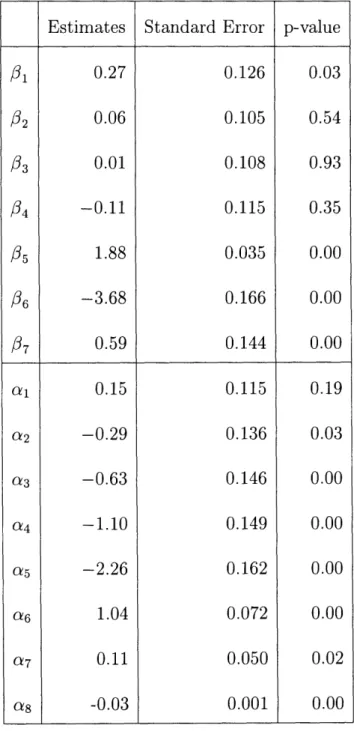
We use Maximum likelihood estimation and the results are reported in the follow-ing table.

Table 6.1: Estimates of 1,.. ., P7 and al,... , 8 Estimates 0.27 0.06 0.01

-0.11

-3.68

-0.29

-0.63

-1.10

-2.26

/3

---

6.1 Estimates of coefficients not related with

9-endings

The sign of coefficients are listed below.

35 > 0: People tend to buy products which they prefer;

p6 < 0: People tend to buy products which are relatively cheaper in that category;

p7

> 0: High-90-endings

attract customers;

a6 > 0: If a person has no personal preference for any items within a category, she

would tend to "not buy";

a7 > 0: If the general prices in a category are high, people tend to choose to "not

buy";

as < 0: People with high budget tend to "purchase" instead of "not buy".

6.2

Estimates for 9-ending effects

As we have known, the within category 9-ending effect is shown in /l, 2,/03 and P4

and the categorical-purchase-stimulation effect is shown in al, a2, a3, a04 and a5.

We can see that

/1

estimate becomes from significant to insignificant. The results show that 9-ending has positive effect on helping an item to stand out or be chosen but this effect decreases when more items have it.

We also see that

cal

the estimates

< 0 and

significant; and al > 0 but insignificant. It implies that 9-ending does have a purchase

stimulation effect1 and this effect grows as more items in a category have 9-endings. We plotted P, ..., P4 and al, ..., a5 as Box plots (Figure 6-1 and Figure 6-2). The

centers of the boxes are the estimates and the bounds are estimates i the standard errors and twices of them.

42 03 .0.0

rIUI,--goP

t

PI,-. I P4P

Chapter 7

Extension and Discussion

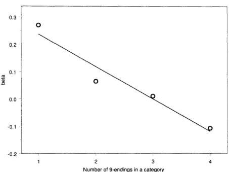
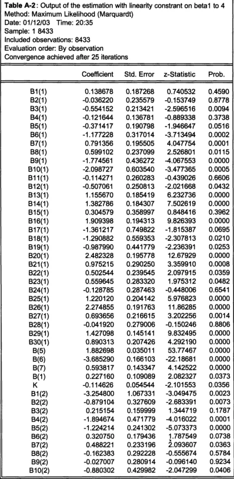
7.1 Linear 9-ending within-category effect

In our previous specification, we use one dummy for each number of 9-counts. So we have four coefficients for the 9-ending within-category effect: P/, P2, P3, P4 to capture

the (decreasing) effect of 9-endings on items with them. Now we are interested to see if the effect decreases linearly. First we draw a picture of linear fit for these Oi's (Figure 7-1).

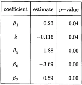
It looks like the change of effects is linear. So we let /2 = 1 + k, 3 = 1 + 2k,

0.3

O

1 2 3 4

Number of 9-endings in a category

Figure 7-1: Linear Fit for , /2, 3 and 34

a, .0 0.2 0.1 0.0 -0.1 O "" -U.,

Table 7.1: Estimates of s and

k

We did an LR test.

-2(log

- log XA) = -2(-10248.30 + 10248.04)

= 0.52

Since X2, 5% = 5.99, We accept the hypothesis of linearity. This result means that as the number of 9-endings in a category increases, its effect on making an item conspicuous drops down linearly.

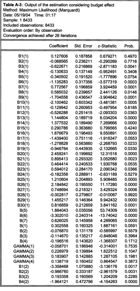
7.2 Effect of budget on the effectiveness of 9-endings

coefficient estimate p-value

f1 0.23 0.04

k -0.115 0.04

/5 1.88 0.00

/6 -3.69 0.00

less careful about prices and they would be more likely to truncate them and un-derestimate price. Consequently they are more likely to buy when more items have 9-endings. However, on the other hand, people with high budget are less bargain prone. Consequently, they are less susceptible to the perception of low prices and image of bargains. So items with endings and categories with high fraction of 9-ending items are less attractive for them. Therefore, we cannot a priori figure out the impact of budget on 9-ending effects without resort to data.

To study this issue, we introduced the dummy for low and high budgets, dummyb, which is 0 if the budget is $40 and 1 if it is $80. The random utility specification now becomes:

= / okjdkj

+

+

if j

and

Uik6

/ 5Zikj /36Pikj + 7hikj +

fyldummyb.

?

%y

?y

= 1,2,3,4,5;

- oldnnlik + a2dnn2ik + ao3dnn3ik + a4dnn4ik + ao5dnn5ik +

ao6ik +- C7Pk +

asqi +

6ldummyb.

dnnlik

dummyb

(7.1)

(7.2)

63dummyb dnn3ik + 64dummyb dnn4ik + 65dummyb dnn5ik + Eik6

ifj

= 6.

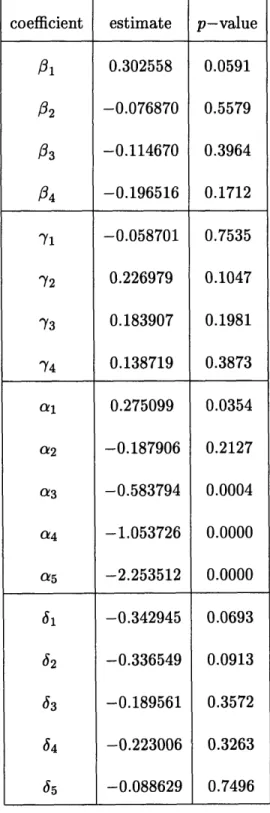
The estimates and p-values are as follows.

Now we are testing whether the higher budget has any impact on 9-endings' within

category effect.

Ho : Y1 = 72 = 73 = 74 = 0

H1 At least one y is not 0.

We still employ an LR test. Because -2(log AR - log Au) = 5.26 < 9.49 = X2

It shows that 9-endings' within category effect is not significantly stronger/weaker for people with higher budget.

We can also test whether higher budget has positive impact on 9-endings'

categorical-purchase-stimulation effect.

Ho: 61 = 2 = 3 = 64 = 65 = 0

H1: At least one 6 is not 0.

The likelihood ratio statistic is 6.32 < 11.07 = X . Therefore 9-endings do

not have significantly stronger or weaker categorical-purchase-stimulation effect for customers with higher budget either.

We can also do a joint test:

The LR statistic, LR = 2(10248.04 - 10242.25) = 11.58 < 16.92 = X2 . There-fore we keep our earlier specification for ikj, j = 1, ..., _{6 (i.e. drop all y's and 's).}

Table 7.2: Estimates of P is considered

,..,

f4

and al,...,a5

coefficient estimate p-value

01 0.302558 0.0591 I82 -0.076870 0.5579 03 -0.114670 0.3964 /34 -0.196516 0.1712 Y1 -0.058701 0.7535 Y2 0.226979 0.1047 Y3 0.183907 0.1981 Y4 0.138719 0.3873 al 0.275099 0.0354 a2 -0.187906 0.2127 a3 -0.583794 0.0004 a4 -1.053726 0.0000 a5 -2.253512 0.0000 61 -0.342945 0.0693 62 -0.336549 0.0913 63 -0.189561 0.3572 64 -0.223006 0.3263 65 -0.088629 0.7496

Chapter 8

Conclusion

The study of price endings, especially nine-endings, has gained increasing attention because of the high fraction of prices which end with nine in the market. For example,

grocery stores now set almost all prices with nine-endings. In other department stores like Walmart, a large number of products have nine-endings but not all. Previous studies have shown that products with nine-ending prices have higher likelihood of purchase than ones with non-nine-ending prices. At the same time, past studies also suggested that a high fraction of nine-ending products decreases the positive effects of nine-endings.

In this paper we developed a theoretical model for prices with 9-ending. It suggests that, in equilibrium, 9 should be set as the price-ending for products with high price

sensitivity.

Our empirical analysis is based on a unique experimental data set developed by Lau (2000). This is in contrast to a scanner data set that might be collected in a typical grocery store today. Many supermarkets have almost all of their prices ending in 9. Such lack of variation makes econometric estimation of 9 effects very difficult.

The experimental results show that a product with a 9-ending is more likely to be chosen than the same product without, but the effect becomes less as more products in the category have 9s. This is consistent with previous research.

Furthermore the experiment finds that increasing the fraction of 9-endings in the category increases the sales in the category. This lends support to the current practice in many stores of using almost all 9-endings.

Appendix A

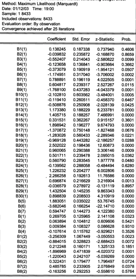
Output of Estimations

The estimation is implemented by EVIEWS codes. In the output, "B" means /, "A" means ca, "GAMMA" means y and "DELTA" means . Particularly, B15(2) means the intercept for Product 2 in Category 15, that is, 0,15,2; B(2) means 02; A(3) means

a3; GAMMA(4) means 74; and DELTA(5) means 65.

The first table is the output of the estimation without considering the effect of different budget, the second is the output of the estimation with the linearity con-straint on p1,. .. 4, and the third is the output of the estimation considering the budget effect.

Table A-I: Output of the estimation without considering budget effect

Method: Maximum Likelihood (Marquardt) Date: 01/12/03 Time: 19:00

Sample: 1 8433

Included observations: 8433

Evaluation order: By observation

Convergence achieved after 25 iterations

Coefficient Std. Error z-Statistic Prob.

B1(1) 0.138245 0.187338 0.737940 0.4606 B2(1) -0.039832 0.235872 -0.168870 0.8659 B3(1) -0.552407 0.214043 -2.580822 0.0099 B4(1) -0.123658 0.136841 -0.903664 0.3662 B5(1) -0.373079 0.190919 -1.954121 0.0507 B6(1) -1.174951 0.317040 -3.706002 0.0002 B7(1) 0.788891 0.196119 4.022505 0.0001 B8(1) 0.604817 0.239317 2.527267 0.0115 B9(1) -1.768100 0.437283 -4.043379 0.0001 B10(1) -2.102810 0.603562 -3.484001 0.0005 B11(1) -0.119410 0.260511 -0.458370 0.6467 B12(1) -0.508876 0.250908 -2.028139 0.0425 B13(1) 1.173380 0.188229 6.233781 0.0000 B14(1) 1.405715 0.188257 7.466991 0.0000 B15(1) 0.331531 0.362267 0.915157 0.3601 B16(1) 1.898942 0.196277 9.674793 0.0000 B17(1) -1.370872 0.750148 -1.827468 0.0676 B18(1) -1.283026 0.560433 -2.289346 0.0221 B19(1) -0.969128 0.443282 -2.186257 0.0288 B20(1) 2.502022 0.198436 12.60873 0.0000 B21(1) 0.960065 0.290388 3.306146 0.0009 B22(1) 0.501711 0.239478 2.095015 0.0362 B23(1) 0.560790 0.283545 1.977778 0.0480 B24(1) -0.139562 0.288058 -0.484494 0.6280 B25(1) 1.226232 0.204277 6.002806 0.0000 B26(1) 2.266258 0.192613 11.76586 0.0000 B27(1) 0.696874 0.216629 3.216904 0.0013 B28(1) -0.036579 0.278972 -0.131119 0.8957 B29(1) 1.432504 0.145235 9.863343 0.0000 B30(1) 0.898839 0.208503 4.310919 0.0000 B(5) 1.883051 0.035022 53.76745 0.0000 B(6) -3.682046 0.166254 -22.14710 0.0000 B(7) 0.594747 0.144273 4.122380 0.0000 B(1) 0.269705 0.125965 2.141108 0.0323 B(2) 0.063894 0.104812 0.609606 0.5421 B(3) 0.009384 0.108327 0.086628 0.9310 B(4) -0.107614 0.115762 -0.929621 0.3526 B1 (2) -3.256309 1.067449 -3.050553 0.0023 B2(2) -0.884015 0.328823 -2.688423 0.0072 B3(2) 0.212248 0.160171 1.325133 0.1851 B4(2) -1.896969 0.471839 -4.020372 0.0001 B5(2) -1.220043 0.242107 -5.039269 0.0000 B6(2) 0.322431 0.179477 1.796497 0.0724

B9(2) B10(2) B11(2) B12(2) B13(2) B14(2) B15(2) B16(2) B17(2) B18(2) B19(2) B20(2) B21(2) B22(2) B23(2) B24(2) B25(2) B26(2) B27(2) B28(2) B29(2) B30(2) B1(3) B2(3) B3(3) B4(3) B5(3) B6(3) B7(3) B8(3) B9(3) B10(3) B11(3) B12(3) B13(3) B14(3) B15(3) B16(3) B17(3) B18(3) B19(3) B20(3) B21(3) B22(3) B23(3) B24(3) B25(3) B26(3) B27(3) B28(3) B29(3) B30(3) B1(4) -0.030154 -0.884627 0.327447 -0.514647 0.900850 -2.008235 -0.134681 0.489612 -2.355672 0.285785 0.298641 1.316245 2.289949 -0.598086 0.654967 0.926771 1.070459 1.382370 0.169393 0.797047 -0.314917 0.200102 -1.001954 0.030892 -0.847512 -0.660563 -0.836561 -2.522353 0.181627 0.872211 -1.218219 0.878033 0.987513 -2.002804 -0.173484 2.426729 -0.762446 0.267816 1.088347 0.258037 1.722451 0.506141 0.155267 1.119581 1.261676 2.050735 0.490287 -0.651651 -1.210893 1.568319 0.153616 -0.680979 -1.873465 0.365514 0.281454 0.429978 0.274394 0.256353 0.224204 0.603350 0.383140 0.289330 1.009061 0.213430 0.283762 0.204891 0.169119 0.391651 0.223100 0.231013 0.208634 0.292209 0.318453 0.252398 0.310139 0.325673 0.297684 0.211533 0.233625 0.292729 0.273302 1.014303 0.255157 0.187224 0.451695 0.195585 0.193383 0.533295 0.250065 0.247512 0.325707 0.172704 0.184158 0.181830 0.204521 0.212498 0.377245 0.184533 0.222717 0.185110 0.295634 0.323814 0.558443 0.152853 0.282724 0.386158 0.646486 0.164417 -0.107137 -2.057376 1.193345 -2.007570 4.017992 -3.328475 -0.351519 1.692228 -2.334520 1.339010 1.052436 6.424121 13.54049 -1.527089 2.935753 4.011765 5.130806 4.730753 0.531925 3.157897 -1.015407 0.614427 -3.365830 0.146038 -3.627667 -2.256568 -3.060937 -2.486785 0.711823 4.658660 -2.696996 4.489273 5.106524 -3.755530 -0.693757 9.804491 -2.340899 1.550723 5.909859 1.419115 8.421861 2.381868 0.411582 6.067097 5.664927 11.07847 1.658427 -2.012422 -2.168337 10.26029 0.543344 -1.763472 -2.897919 2.223089 0.9147 0.0397 0.2327 0.0447 0.0001 0.0009 0.7252 0.0906 0.0196 0.1806 0.2926 0.0000 0.0000 0.1267 0.0033 0.0001 0.0000 0.0000 0.5948 0.0016 0.3099 0.5389 0.0008 0.8839 0.0003 0.0240 0.0022 0.0129 0.4766 0.0000 0.0070 0.0000 0.0000 0.0002 0.4878 0.0000 0.0192 0.1210 0.0000 0.1559 0.0000 0.0172 0.6806 0.0000 0.0000 0.0000 0.0972 0.0442 0.0301 0.0000 0.5869 0.0778 0.0038 0.0262

B4(4) B5(4) B6(4) B7(4) B8(4) B9(4) B10(4) B11(4) B12(4) B13(4) B14(4) B15(4) B16(4) B17(4) B18(4) B19(4) B20(4) B21(4) B22(4) B23(4) B24(4) B25(4) B26(4) B27(4) B28(4) B29(4) B30(4) A(6) A(7) A(8) A(1) A(2) A(3) A(4) A(5) -1.401880 -1.559495 0.751891 -0.749017 1.265246 -1.345509 -1.487371 0.713014 0.056947 -0.032617 0.023811 1.925940 -1.096371 -0.687668 1.473179 1.353060 -1.099285 0.110184 2.699346 0.600877 -0.341007 0.774771 0.607490 0.645069 -0.046038 -0.467009 0.364776 1.035877 0.112922 -0.029344 0.151677 -0.287077 -0.626223 -1.100726 -2.264701 0.287408 0.378890 0.219235 0.256229 0.184557 0.455051 0.424512 0.196915 0.205886 0.259585 0.209478 0.174022 0.448354 0.255725 0.225122 0.159459 1.014380 0.259237 0.213745 0.275123 0.395287 0.237657 0.183544 0.267271 0.331975 0.440959 0.218121 0.071731 0.050085 0.001359 0.114991 0.135727 0.145801 0.149491 0.161590 -4.877663 -4.115959 3.429609 -2.923230 6.855577 -2.956830 -3.503716 3.620925 0.276597 -0.125651 0.113667 11.06724 -2.445322 -2.689089 6.543930 8.485316 -1.083701 0.425031 12.62883 2.184031 -0.862682 3.260033 3.309777 2.413541 -0.138680 -1.059076 1.672357 14.44111 2.254596 -21.58691 1.319035 -2.115110 -4.295053 -7.363165 -14.01511 0.0000 0.0000 0.0006 0.0035 0.0000 0.0031 0.0005 0.0003 0.7821 0.9000 0.9095 0.0000 0.0145 0.0072 0.0000 0.0000 0.2785 0.6708 0.0000 0.0290 0.3883 0.0011 0.0009 0.0158 0.8897 0.2896 0.0945 0.0000 0.0242 0.0000 0.1872 0.0344 0.0000 0.0000 0.0000

Log likelihood -10248.04 Akaike info criterion 2.462478 Avg. log likelihood -1.215230 Schwarz criterion 2.575176

Table A-2: Output of the estimation with linearity constrant on beta1 to 4

Method: Maximum Likelihood (Marquardt) Date: 01/12/03 Time: 20:35

Sample: 1 8433

Included observations: 8433 Evaluation order: By observation

Convergence achieved after 25 iterations

Coefficient Std. Error z-Statistic Prob.

B1(1) 0.138678 0.187268 0.740532 0.4590 B2(1) -0.036220 0.235579 -0.153749 0.8778 B3(1) -0.554152 0.213421 -2.596516 0.0094 B4(1) -0.121644 0.136781 -0.889338 0.3738 B5(1) -0.371417 0.190798 -1.946647 0.0516 B6(1) -1.177228 0.317014 -3.713494 0.0002 B7(1) 0.791356 0.195505 4.047754 0.0001 B8(1) 0.599102 0.237099 2.526801 0.0115 B9(1) -1.774561 0.436272 -4.067553 0.0000 B10(1) -2.098727 0.603540 -3.477365 0.0005 B1(1) -0.114271 0.260283 -0.439026 0.6606 B12(1) -0.507061 0.250813 -2.021668 0.0432 B13(1) 1.155670 0.185419 6.232736 0.0000 B14(1) 1.382786 0.184307 7.502619 0.0000 B15(1) 0.304579 0.358997 0.848416 0.3962 B16(1) 1.909398 0.194313 9.826393 0.0000 B17(1) -1.361217 0.749822 -1.815387 0.0695 B18(1) -1.290882 0.559353 -2.307813 0.0210 B19(1) -0.987990 0.441779 -2.236391 0.0253 B20(1) 2.482328 0.195778 12.67929 0.0000 B21(1) 0.975215 0.290250 3.359910 0.0008 B22(1) 0.502544 0.239545 2.097915 0.0359 B23(1) 0.559645 0.283320 1.975312 0.0482 B24(1) -0.128785 0.287463 -0.448006 0.6541 B25(1) 1.220120 0.204142 5.976823 0.0000 B26(1) 2.274855 0.191763 11.86285 0.0000 B27(1) 0.693656 0.216615 3.202256 0.0014 B28(1) -0.041920 0.279006 -0.150246 0.8806 B29(1) 1.427098 0.145141 9.832495 0.0000 B30(1) 0.890313 0.207426 4.292190 0.0000 B(5) 1.882698 0.035011 53.77467 0.0000 B(6) -3.685290 0.166103 -22.18681 0.0000 B(7) 0.593817 0.143347 4.142522 0.0000 B(1) 0.227160 0.109089 2.082327 0.0373 K -0.114626 0.054544 -2.101553 0.0356 1B1(2) -3.254800 1.067331 -3.049475 0.0023 B2(2) -0.879104 0.327609 -2.683391 0.0073 B3(2) 0.215154 0.159999 1.344719 0.1787 B4(2) -1.894674 0.471779 -4.016022 0.0001 B5(2) -1.224214 0.241302 -5.073373 0.0000 B6(2) 0.320750 0.179436 1.787549 0.0738 B7(2) 0.488221 0.233196 2.093607 0.0363 B8(2) -0.162383 0.292228 -0.555674 0.5784

B11(2) B12(2) B13(2) B14(2) B15(2) B16(2) B17(2) B18(2) B19(2) B20(2) B21(2) B22(2) B23(2) B24(2) B25(2) B26(2) B27(2) B28(2) B29(2) B30(2) B1(3) B2(3) B3(3) B4(3) B5(3) B6(3) B7(3) B8(3) B9(3) B10(3) B11(3) B12(3) B13(3) B14(3) B15(3) B16(3) B17(3) B18(3) B19(3) B20(3) B21(3) B22(3) B23(3) B24(3) B25(3) B26(3) B27(3) B28(3) B29(3) B30(3) B1(4) B2(4) B3(4) 0.326528 -0.522863 0.883398 -2.008783 -0.135523 0.480959 -2.378163 0.302758 0.296913 1.316202 2.291109 -0.596828 0.633651 0.928517 1.064376 1.392210 0.166372 0.812911 -0.303220 0.190997 -1.007322 0.034881 -0.845340 -0.661864 -0.833244 -2.523965 0.183903 0.862548 -1.226161 0.882571 0.981919 -2.006552 -0.169576 2.404558 -0.765447 0.283958 1.093036 0.269068 1.704080 0.506636 0.157723 1.120156 1.262022 2.030800 0.504231 -0.642545 -1.213969 1.562461 0.148693 -0.690547 -1.872912 0.368527 -1.586382 0.272161 0.255567 0.221620 0.602163 0.382957 0.288457 1.007739 0.211147 0.282888 0.204858 0.168984 0.391562 0.220763 0.230387 0.208503 0.291350 0.318593 0.250381 0.310186 0.324610 0.297207 0.211152 0.233571 0.292566 0.272275 1.014300 0.254153 0.186480 0.451538 0.194699 0.192953 0.532532 0.248780 0.245353 0.324740 0.171431 0.183726 0.179870 0.201829 0.212129 0.377315 0.184227 0.222068 0.183347 0.293802 0.323085 0.558489 0.152722 0.282710 0.385693 0.646428 0.163959 0.495356 1.199762 -2.045894 3.986104 -3.335948 -0.353886 1.667353 -2.359900 1.433874 1.049577 6.424950 13.55813 -1.524223 2.870282 4.030256 5.104847 4.778478 0.522208 3.246703 -0.977543 0.588390 -3.389298 0.165193 -3.619201 -2.262272 -3.060305 -2.488381 0.723590 4.625423 -2.715522 4.533006 5.088895 -3.767946 -0.681631 9.800387 -2.357111 1.656398 5.949284 1.495903 8.443187 2.388340 0.418013 6.080312 5.683048 11.07624 1.716228 -1.988778 -2.173666 10.23075 0.525956 -1.790404 -2.897325 2.247682 -3.202513 0.2302 0.0408 0.0001 0.0009 0.7234 0.0954 0.0183 0.1516 0.2939 0.0000 0.0000 0.1275 0.0041 0.0001 0.0000 0.0000 0.6015 0.0012 0.3283 0.5563 0.0007 0.8688 0.0003 0.0237 0.0022 0.0128 0.4693 0.0000 0.0066 0.0000 0.0000 0.0002 0.4955 0.0000 0.0184 0.0976 0.0000 0.1347 0.0000 0.0169 0.6759 0.0000 0.0000 0.0000 0.0861 0.0467 0.0297 0.0000 0.5989 0.0734 0.0038 0.0246 0.0014

B6(4) 0.745009 0.218501 3.409628 0.0007 B7(4) -0.757166 0.255929 -2.958495 0.0031 B8(4) 1.266572 0.184203 6.875977 0.0000 B9(4) -1.342448 0.454431 -2.954131 0.0031 B10(4) -1.486769 0.423226 -3.512942 0.0004 B11(4) 0.718200 0.196741 3.650488 0.0003 B12(4) 0.058702 0.205292 0.285945 0.7749 B13(4) -0.021627 0.259353 -0.083388 0.9335 B14(4) 0.023314 0.208622 0.111751 0.9110 B15(4) 1.924164 0.173801 11.07108 0.0000 B16(4) -1.086222 0.447767 -2.425863 0.0153 B17(4) -0.713566 0.251800 -2.833855 0.0046 B18(4) 1.486088 0.221115 6.720892 0.0000 B19(4) 1.351537 0.157119 8.601973 0.0000 B20(4) -1.089015 1.012726 -1.075330 0.2822 B21(4) 0.093009 0.257674 0.360955 0.7181 B22(4) 2.678062 0.211180 12.68140 0.0000 B23(4) 0.601032 0.275021 2.185403 0.0289 B24(4) -0.342103 0.395156 -0.865743 0.3866 B25(4) 0.768545 0.237617 3.234378 0.0012 B26(4) 0.621942 0.183266 3.393651 0.0007 B27(4) 0.659612 0.266210 2.477785 0.0132 B28(4) -0.051186 0.331954 -0.154197 0.8775 B29(4) -0.471797 0.440952 -1.069952 0.2846 B30(4) 0.357080 0.217136 1.644496 0.1001 A(6) 1.036442 0.071696 14.45598 0.0000 A(7) 0.110427 0.049959 2.210342 0.0271 A(8) -0.029352 0.001359 -21.59705 0.0000 A(1) 0.144745 0.114338 1.265944 0.2055 A(2) -0.268379 0.133617 -2.008571 0.0446 A(3) -0.629716 0.139636 -4.509697 0.0000 A(4) -1.104965 0.146378 -7.548694 0.0000 A(5) -2.262424 0.161551 -14.00442 0.0000

Log likelihood -10248.30 Akaike info criterion 2.462065 Avg. log likelihood -1.215261 Schwarz criterion 2.573094 Number of Coefs. 133 Hannan-Quinn criter. 2.499968

Table A-3: Output of the estimation considering budget effect

Method: Maximum Likelihood (Marquardt) Date: 05/19/04 Time: 01:17

Sample: 1 8433

Included observations: 8433 Evaluation order: By observation

Convergence achieved after 26 iterations

Coefficient Std. Error z-Statistic Prob.

B1(1) 0.127606 0.187858 0.679271 0.4970 B2(1) -0.068565 0.236211 -0.290269 0.7716 B3(1) -0.622671 0.216869 -2.871183 0.0041 B4(1) -0.130633 0.137149 -0.952491 0.3408 B5(1) -0.340502 0.191520 -1.777896 0.0754 B6(1) -1.135283 0.317356 -3.577319 0.0003 B7(1) 0.772567 0.196859 3.924459 0.0001 B8(1) 0.585032 0.239657 2.441126 0.0146 B9(1) -1.704558 0.436547 -3.904642 0.0001 B10(1) -2.100462 0.603342 -3.481381 0.0005 B11(1) -0.129942 0.260953 -0.497954 0.6185 B12(1) -0.526288 0.251415 -2.093303 0.0363 B13(1) 1.144804 0.189719 6.034204 0.0000 B14(1) 1.377532 0.189490 7.269666 0.0000 B15(1) 0.290786 0.363680 0.799565 0.4240 B16(1) 1.876679 0.196493 9.550891 0.0000 B17(1) -1.439400 0.751116 -1.916347 0.0553 B18(1) -1.278828 0.563660 -2.268793 0.0233 B19(1) -0.946764 0.443935 -2.132665 0.0330 B20(1) 2.459241 0.199692 12.31518 0.0000 B21 (1) 0.895413 0.293320 3.052680 0.0023 B22(1) 0.464414 0.240533 1.930768 0.0535 B23(1) 0.594012 0.284170 2.090342 0.0366 B24(1) -0.182358 0.288911 -0.631189 0.5279 B25(1) 1.210604 0.204893 5.908485 0.0000 B26(1) 2.184842 0.195550 11.17280 0.0000 B27(1) 0.748694 0.218321 3.429324 0.0006 B28(1) -0.002817 0.279807 -0.010067 0.9920 B29(1) 1.455217 0.146364 9.942432 0.0000 B30(1) 0.816859 0.212659 3.841162 0.0001 B(5) 1.884043 0.035056 53.74309 0.0000 B(6) -3.302010 0.240314 -13.74042 0.0000 B(7) 0.626025 0.145958 4.289065 0.0000 B(1) 0.302558 0.160325 1.887161 0.0591 B(2) -0.076870 0.131178 -0.585997 0.5579 B(3) -0.114670 0.135217 -0.848046 0.3964 B(4) -0.196516 0.143620 -1.368307 0.1712 GAMMA(1) -0.058701 0.186946 -0.314001 0.7535 GAMMA(2) 0.226979 0.139894 1.622512 0.1047 GAMMA(3) 0.183907 0.142885 1.287105 0.1981 GAMMA(4) 0.138719 0.160452 0.864547 0.3873 B1(2) -3.358468 1.070880 -3.136176 0.0017 B2(2) -0.986760 0.333187 -2.961579 0.0031 B3(2) 0.193358 0.160569 1.204209 0.2285 B4(2) -1.964121 0.472796 -4.154263 0.0000