Publisher’s version / Version de l'éditeur:
International Journal of Prognostics and Health Management, 5, 2, pp. 1-11,
2015-01-28
READ THESE TERMS AND CONDITIONS CAREFULLY BEFORE USING THIS WEBSITE.
https://nrc-publications.canada.ca/eng/copyright
Vous avez des questions? Nous pouvons vous aider. Pour communiquer directement avec un auteur, consultez la première page de la revue dans laquelle son article a été publié afin de trouver ses coordonnées. Si vous n’arrivez pas à les repérer, communiquez avec nous à [email protected].
Questions? Contact the NRC Publications Archive team at
[email protected]. If you wish to email the authors directly, please see the first page of the publication for their contact information.
Archives des publications du CNRC
This publication could be one of several versions: author’s original, accepted manuscript or the publisher’s version. / La version de cette publication peut être l’une des suivantes : la version prépublication de l’auteur, la version acceptée du manuscrit ou la version de l’éditeur.
Access and use of this website and the material on it are subject to the Terms and Conditions set forth at
Predictive model evaluation for PHM
Yang, Chunsheng; Zou, Yanni; Liu, Jie; Mulligan, Kyle R.
https://publications-cnrc.canada.ca/fra/droits
L’accès à ce site Web et l’utilisation de son contenu sont assujettis aux conditions présentées dans le site
LISEZ CES CONDITIONS ATTENTIVEMENT AVANT D’UTILISER CE SITE WEB.
NRC Publications Record / Notice d'Archives des publications de CNRC:
https://nrc-publications.canada.ca/eng/view/object/?id=dce076fe-03db-4d8c-b097-5ca015aa414d
https://publications-cnrc.canada.ca/fra/voir/objet/?id=dce076fe-03db-4d8c-b097-5ca015aa414d
Chunsheng Yang1, Yanni Zou2, Jie Liu3 , Kyle R Mulligan4
1National Research Council Canada, Ottawa, Ontario K1A 0R6, Canada
2
Jiujiang University, Jiangxi, China [email protected]
3
Dept. of Mechanical and Aerospace Eng., Carleton University, Ottawa, ON, K1S 5B6, Canada [email protected]
4GAUS, Dept. of Mechanical Engineering, Universit´e de Sherbrooke, Sherbrooke, QC, J1K 2R1, Canada
ABSTRACT
In the past decades, machine learning techniques or algorithms, particularly, classifiers have been widely applied to various real-world applications such as PHM. In developing high-performance classifiers, or machine learning-based models, i.e. predictive model for PHM, the predictive model evaluation remains a challenge. Generic methods such as accuracy may not fully meet the needs of models evaluation for prognostic applications. This paper addresses this issue from the point of view of PHM systems. Generic methods are first reviewed while outlining their limitations or deficiencies with respect to PHM. Then, two approaches developed for evaluating predictive models are presented with emphasis on specificities and requirements of PHM. A case of real prognostic application is studies to demonstrate the usefulness of two proposed methods for predictive model evaluation. We argue that predictive models for PHM must be evaluated not only using generic methods, but also domain-oriented approaches in order to deploy the models in real-world applications.
Keyword: Machine Learning Algorithms, Predictive Models Evaluation, Generic Methods, Binary Classifier, Prognostics and Health Management (PHM), Prognostics, Time to Failure
1. INTRODUCTION
One of the objectives of Prognostics and Health Management (PHM) systems is to help reduce the number of unexpected failures by continuously monitoring the components of interest and predicting their failures
sufficiently in advance to allow for proper planning of maintenance. The core of PHM is prognostics, which is defined as an emerging technique being able to predict failure before it happened and to precisely estimate remaining useful life (RUL) or time to failure (TTF) (Jardine 2006, Schwabacher 2007). For the failure prediction, one effective way is to develop predictive models to predict failures. Recently, a data-driven predictive modeling attracts much attention from researchers in machine learning community. This modeling technique is to develop classifiers using classification algorithms, such a classifier is able to classify the system operation statues into “normal (negative)” or “abnormal (positive)”. Usually, the positive status is used as an alert for failure predictions. For example, Yang (2005) developed predictive models (binary classifiers) from the historical operation and maintenance data to predict train wheel failure. The ultimate goal of prognostics is to predict the probability of a failure and precisely estimate its TTF for a monitored component/subsystem in complex systems. This can be done by developing numeric prognostic models, either data-drive models or knowledge-based models. Due to specificities of prognostics, evaluation of prognostic methods/models is much more challenge. Recently, some researchers started to look into the performance evaluation of prognostic methods. Saxena et al (2014, 2009) investigated the evaluation metrics for comparing the performance of prognostic methods by focusing on the RUL estimation-based prognostics models. In their work, they proposed to evaluate prognostic methods/algorithms in online and offline running environments, and suggested some metrics such as respond time, prediction horizon and accuracy. Such metrics are useful for computing regression-based RUL estimation models. However, it is still difficult to compute the performance of predictive models because those metrics are designed for numeric models, not for discrete classification-based models. Our paper addresses this issue by focusing on performance evaluation of predictive models in offline running environment. In ____________________
Chunsheng Yang, et.al. This is an open-access article distributed under the terms of the Creative Commons Attribution 3.0 United States License, which permits unrestricted use, distribution, and reproduction in any medium, provided the original author and source are credited.
general, the offline environment can provide the ground truth for evaluation. We believe that the evaluation of predictive models can be treated as classifier evaluation from the point of view of machine learning (we will use term “model” and “classifier” alternatively later in this paper). It is desirable that such a model evaluation not only helps practitioners compute the performance of a model, but also assists them assess business value of a predictive model. The ideal way to evaluate predictive models is to perform field trials in real-world environments. This is, however, unrealistic and costly. Existing methods are to compute the performance of models using generic methods available from the machine learning community.
However, these generic evaluation approaches sometimes fail to take specificities of PHM applications into consideration, and thus may not satisfy the needs of predictive model evaluation for PHM. To evaluate effectively predictive models, the metrics have to take the TTF and failure coverage into consideration (detailed in Section 4). Unfortunately, to our best knowledge, none of the existing generic methods do so. In order to improve generic methods for evaluating prognostic models, domain-oriented approaches, which incorporate the specific requirements of domain problems into evaluation metrics by tailoring existing generic methods, are proposed. Prior to this, generic methods are reviewed, and its deficiencies are discussed when applying them to classifier evaluation for fielded applications. Then new approaches developed for prognostic applications are presented. These approaches help developers not only evaluating the model performance, but also identifying the usefulness and business value, which could be achieved once a model is deployed in application. The objective is to emphasize that a predictive model should be carefully evaluated by incorporating PHM specific requirements into evaluation metrics.
The paper is structured to include the following sections: Section 2 reviews generic methods; Section 3 discusses the limitations of generic methods from the point of view of PHM applications; Section 4 presents the approaches developed for evaluating predictive models; Section 5 presents a case study for comparing the evaluation for different methods; and the final Section concludes the paper.
2. OVERVIEW OF GENERIC METHODS
2.1. Preliminaries
One of the most important tasks in classification research is to build classifiers from a given dataset,
}) ... 3 , 2 , 1 { ( } ,
{xk yk nk1 yk m , where m is the number of classes and n is a total number of samples (or instances). The developed classifier
f
(
)
classifies a new datax
k as}) 3 , 2 , 1 { ˆ ( ) ( ˆ f x y m
yk k k . The ultimate goal is to make
k k
y
y
ˆ
by incorporating all kinds of notions of costs, errors, and losses into modeling. To evaluate generalization performance of a classifierf
(
)
, a testing dataset, which is unseen or new data for the classifier, is used. As a result, a confusion matrix can be obtained by running the classifier on the testing dataset. We note this confusion matrix asC
, expressed as Equation 1In Equation 1,
c
ij is the number of misclassified instances, i.e., the number of the instances classified as the ithclass which are really in the jth class. Predicted classes are represented by the rows of the matrix whereas true classes are represented by the columns.An ideal classifier should ultimately generate a confusion matrix in which
c
ij ,
0
i
j
by incorporating noise and errors in classification. Using this confusion matrix, the performance of a classifier can be computed. Over the past decades, generic methods have been developed from the confusion matrix. Generally speaking, generic methods can be grouped into scoring methods and graphical methods. In the following subsections, these generic methods are reviewed.2.2. Scoring methods
The scoring metrics includes Accuracy (or Error Rate), True Positive Rate(TPR), False Positive Rate(FNR), True Negative Rate (TNR), False Negative Rate (FNR), Sensitivity, Specificity, Recall, Precision, and F-Score. These metrics (Japkowicz and Shah 2011) provide a simple and effective way to measure the performance of a classifier. To simplify the definitions and notations, these metrics are illustrated using binary classification, i.e., m = 2, and
y
k
{
1
,
1
}
. For binary classification, the confusion matrix in Equation 1 is simplified as a 2x2 matrix shown in Equation 2.)
1
(
2 1 1 2 22 21 1 12 11
mm m m im ii i m mc
c
c
c
c
c
c
c
c
c
c
c
C
)
2
(
22 21 12 11
c
c
c
c
C
where:
c11 is the number of true positives;
c12 is the number of false positives;
c21 is the number of false negatives; and
c22 is the number of true negatives.
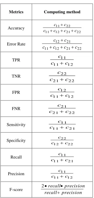
Table 1. The scoring metrics
Metrics Computing method
Accuracy 22 21 12 11 22 11 c c c c c c Error Rate 22 21 12 11 21 12
c
c
c
c
c
c
TPR 12 11 11c
c
c
TNR 22 21 22c
c
c
FPR 1 2 1 1 1 2 c c c FNR 2 2 2 1 2 1 c c c Sensitivity 2 1 1 1 1 1 c c c Specificity 2 2 1 2 2 2 c c c Recall 2 1 1 1 1 1 c c c Precision 1 2 1 1 1 1 c c c F-score precision recall precision recall 2From this confusion matrix, scoring metrics are computed as shown in Table 1. These scoring metrics are widely used in comparing or ranking the performance of classifiers because they are simple, compute, and
easy-to-understand. Such an evaluation typically examines unbiased estimates of predictive accuracy of different classifiers (Srinivasan 1999). The assumption is that the estimates of performance are subject to sampling errors only and that the classifier with the highest accuracy would be the “best” choice of the classifiers for a given problem. These metrics overlook two important practical concerns: class distribution and the cost of misclassification. For example, the accuracy metric assumes that the class distribution is known in the training dataset and testing dataset and that the misclassification costs for false positive and false negative error are equal (Provost 1998). In real-world application, the cost of misclassification for different errors may not be the same. It is sometimes desirable to minimize the misclassification cost rather than the error-rate in classification task.
2.3. Graphical methods
To overcome the limitations of scoring metrics and incorporate the consideration of prior class distributions and the misclassification costs, several graphical methods had been developed. These graphic methods are ROC (Receiver Operating Characteristics) Space, ROCCH (ROC Convex Hull), Isometrics, AUC (Area under ROC curve), Cost Curve, DEA (Data Envelopment Analysis), and Lift curve. They are also useful for visualizing performance of a classifier. Here is an overview for each method.
2.3.1. ROC Space
The ROC analysis was initially developed to express the tradeoffs between hit rate and false alert rate in signal detection theory (Egan 1975). It is now also used for evaluating classifier performance (Bradley 1997, Provost and Fawcett 2001, 1997). In particular, ROC is a powerful way for performance evaluation of binary classifiers, and it has become a popular method due to its simple graphical representation of overall performance.
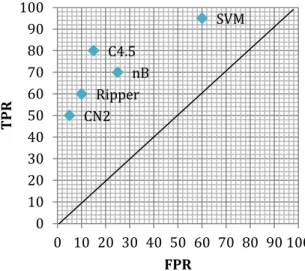
Using TPR and FPR from Table 1 as the Y-axis and X-axis respectively, a ROC space can be plotted. In this ROC space, each point (FPR, TPR) represents a classifier (Fawcett 2003, Flach 2004, 2003). Figure 1 shows an example of a basic ROC graph for five discrete classifiers. Based on the position of a classifier in ROC space, we can evaluate or rank the performance of classifiers. In ROC space, the point (0, 1) represents a perfect classifier which has 100% accuracy and zero error rates. The upper left points indicated that a classifier has a higher TPR and a lower FPR. For instance, C4.5 has a better TPR and a lower FPR than nB. The classifier on the upper right-hand side of an ROC space makes positive classification with relative weak evidence and has a higher TPR and a higher FPR. Therefore, the performance of a classifier is determined by a trade-off between TPR and FPR. However, it is hard to decide which classifier is best from ROC space. For
example, it is difficult to tell which classifier is better for CN2 and nB in Figure 1 (The unit of FPR/TPR axils is %).
2.3.2. ROCCH
As mentioned, ROC space is useful for visualizing the performance of classifiers regardless of class distribution and misclassification costs. In order to further use ROC space to select the optimal classifiers, a useful way is to generate ROCCH (Provost et al. 2003, Bradley 1997). This ROC convex hull represents the best performance that can be achieved by a set of classifiers. The classifiers on ROCCH usually achieve the best accuracy.
Figure 1. A ROC graph for 5 classifiers (Flach 2004)
2.3.3. Isometrics
To further use ROCCH to rank the performance of classifiers, we can add isometrics to ROCCH (Flach 2004, 2003). Isometrics are collections of points with the same value for a given metric (Flach 2003). In ROC space, isometrics are lines. To draw the isometrics for a given metric such as accuracy, the accuracy isometrics can be added to ROCCH using the approach proposed by Flach (2003). In the same way, other metrics isometrics such as precision could also be added to ROCCH in order to decide the optimal classifiers based on precision metric and a given class distribution.
2.3.4. AUC
In ROC space, a ROC curve is plotted for a given classifier by sampling different class proportions of positive and negative samples in the training dataset. A ROC curve is a segment line connecting points in ROC space from left-hand side to right-hand side. Such a ROC curve illustrates the error tradeoffs. It describes the predictive behavior of a classifier independent of class distribution and error costs, so it decouples generalization performance of a classifier from these factors. The area under the ROC curve is
denoted as AUC (Bradley 1997, Huang and Ling 2005). AUC can be used to rank or compare the performance of classifiers. It is more appropriate whenever the class distribution and error costs are unknown because it corresponds to the shape of the entire ROC curve rather than any single point in ROC space (Swets et al. 2003). AUC has been proven more powerful than Accuracy in experimental comparisons of several popular learning algorithms (Huang and Ling 2005).
To compute the AUC for binary classifiers, Hand and Till (2001) proposed a simple formula:
where n0 and n1 are the number of positive and negative
examples respectively, and ri is the rank of the ith positive
example in the ranked list for all examples in the test dataset.
2.3.5. Cost curve
The cost curve is a graphical representation for visualizing binary classifier performance over a full range of possible CN2 Ripper nB C4.5 SVM 0 10 20 30 40 50 60 70 80 90 100 0 10 20 30 40 50 60 70 80 90 100 TPR FPR ) 3 ( ) ( 1 0 1 0 n n i r AUC n i i
1 0.5 False Positive RateFigure 2. A ROC curve with 10 points
Probability of Positive
Figure 3. Cost lines and their lower envelope
E x p ec te d C o st
class distributions and misclassification costs. It transforms a ROC curve or a ROCCH into another two dimensional space using normalized expected costs and probabilities instead of the TPR and FPR. In the cost curve, the y-axis is the expected cost, which is the normalized value of the total misclassification cost, and the x-axis is a probability function, which combines with the cost of a false positive and a false negative. A point (TPR, FPR) in the ROC space can be projected into the cost curve space as a cost line. By projecting a set of points onto the ROC curve into the cost curve space, a set of cost lines can be obtained. The lower envelope of these cost lines forms a cost curve. For example, a ROC curve containing 10 points for a given classifier is shown in Figure 2. The corresponding set of cost lines to 10 points in ROC space is shown in Figure 3 where the lower envelope forms a cost curve for a given classifier. Further details on cost curve construction are described in (Drummond and Holte 2004, 2000A).
2.3.6. DEA
The DEA method is a more effective way for multi-class classifier evaluation. It is widely used in decision-making support and management science. It addresses the key issues in determining the efficiencies of various producers or DMUs (Decision Making Units) by converting a set of inputs into a set of outputs (Banker et al. 1984, Zheng et al. 2004). DEA is a linear programming based approach, which constructs an efficient frontier (envelopment) over the data and computes each data point’s efficiency related to this frontier. Each data point corresponds to a DMU or a producer in applications. Zheng, et al.(2004) has attempted to apply DEA to classifier evaluation. They have proven that DEA and ROCCH have the same convex hull for binary classifications. In other words, DEA is equivalent to ROCCH for binary classification tasks.
2.3.7. Lift curve
The Lift is often used in marketing analysis. It is also useful for classifier evaluation. Lift measures how much better a classifier is at predicting positive than a baseline classifier that randomly predicts positives (Caruana et al. 2006, 2004, Giudici 2003, Prechelt 1996). It is defined as follows:
% %
/ APT
PT
Left
. Here PT% is % of true positives above the given threshold and APT% is % of samples in dataset above the threshold. For example, an agent intends to send advertising to the potential customers but only afford to send ads to 10% of the population and wish these customers will response. How the agent chooses these samples from the populations is a classification problem. A classifier should be trained for predicting positive response customers. A classifier with the maximum Lift will help the agent to get the maximum numbers of the customers who will respond to the advertisement in this dataset.3. ISSUES WITH GENERIC METHODS
Generic approaches, either scoring methods or graphic methods, have played an important role in classifier evaluation. However, there are some limitations. As Salzberg (1997) pointed out, good classifier evaluations are not done nearly enough using datasets from real world problems. For example, in 200 surveyed papers on neural network learning algorithms (Flexer 1996), 29% of these algorithms are not evaluated with any real problem data, and only 8% of these algorithms can be compared with real problem data. Flexer did another survey on 43 neural network papers from leading journals and found that only 3 out of 43 papers used real problem data to test their algorithms or tune the parameters for the algorithms. It is desirable that a classifier should be evaluated carefully not only using right metric but also the right data from real world problems, or so-called fielded applications. However, existing generic methods may not able to validate the performance of classifiers for some real-world problems due to some ingrained deficiencies. The deficiencies with generic evaluation methods can be summarized as follows. First, generic methods request i.i.d. sampling in evaluation. In practice many data from real-world problems may not meet this requirement of instance independency. For example, instances in time-series from prognostic applications are not independent. They are time dependent. The i.i.d. based random sampling may separate dependent data into different groups such as training and testing dataset. In fact, the instances associated with a time series should stay in the same group.
Secondly, generic metrics have some deficiencies themselves. The scoring metrics do not account the cost of misclassification or error rates for evaluation. This is a serious problem because some errors may cost more than others in different problems. For example, in the medical diagnostic application, the false negative for a cancer could cost much more than a false positive.
1
t0
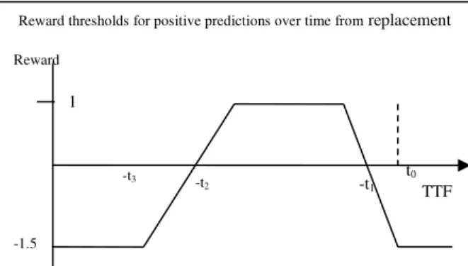
Reward thresholds for positive predictions over time from replacement
Figure 5. A reward function for positivepredictions -1.5 Reward -t1 -t2 -t3 TTF
Thirdly, interpretation of evaluation results from generic metrics may be difficult to tell practitioners meaningful information. In other words, interpretation of evaluating results is hard to understand, even misleading. For example, AUC, a normalized value between 0 and 1, is supposed to address the deficiencies of ROC curve. Theoretically, the higher the AUC value, the better the performance of a classifier. Therefore, a classifier with 0.8 of AUC value should be better than one with 0.75 of AUC value. However, such interpretation may be meaningless or useless for an end user. From the point of view of business value, the interpretation may be totally different. The classifier with 0.8 of AUC value may save $50,000, and the classifier with 0.75 of AUC value may save $60,000 after they are deployed in a real-world application.
Finally, generic methods do not take the specificities or settings of real-world applications into consideration, in particularly, for prognostic applications. As an emerging application of classification to real-world problems, prognostics (Schwabacher and Goebel 2007, Yang and Létourneau 2005)] is to develop the predictive models (classifiers) from large-sized operation and maintenance data by using techniques from machine learning. Such a prognostic model is able to predict the likelihood of a failure with a relatively accurate TTF estimation. Existing generic methods failed to incorporate these specific factors into classifier evaluation.
4. MODEL EVALUATION FOR PROGNOSTICS
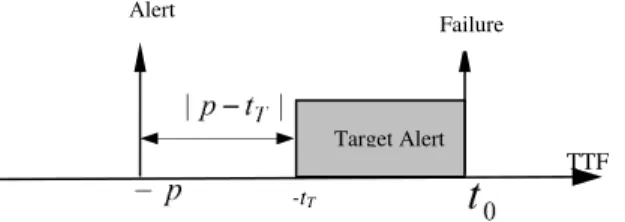
As emphasized above, predictive models evaluation needs to take domain specificities into account. Such specificities cover two aspects: capability of failure prediction and TTF estimation. From the point of view of TTF, it is desirable that a predictive model can generate alerts in a “targeted” time window prior to a failure. A model that predicts a failure too early leads to non-optimal component use. On
the other hand, if the failure prediction is too close to the actual failure then it becomes difficult to schedule an effective maintenance. Figure 4 shows the requirement for prognostic models in the relationship between alert time and TTF. We use tT and t0 to denote the beginning and then end of this target window. The time at which the predictive model predicts a failure (and alert is raised) is noted p.
When p < tT there is a potential for replacing a component before the end of its useful life and therefore losing some component usage. From the point of view of failure predictions, it is expected that a predictive model should be able to predict all potential failures with reasonable number of alerts (positive predictions) instead of few failures within many alerts.
4.1. Score-based approach
To address the specificities of prognostic application and evaluate the performance of predictive models effectively, a score-based approach is proposed by which the problem coverage and TTF is incorporated into classifier evaluation. The score-based method is briefly reviewed in the following.
In the score-based method, a reward function is first defined for predicting the correct instance outcome. The reward for predicting a positive instance is based on time to failure between alert generation and the actual failure, i.e. the determined target window. Figure 5 shows a graph of this function. The time target window is formed as [-t2, -t1]. The
parameters t1 and t2 are determined based on the
requirement of prognostic application. The maximum gain is obtained when the model predicts the failure in the target window prior to a component failure. Outside this target window, predicting a failure can lead to a negative reward threshold. As such a prediction corresponds to misleading advice. Accordingly, false positive predictions (predictions of a failure when there is no failure) are penalized by a reward of -1.5 in comparison to a 1.0 reward for true positive predictions (predictions of failure when there is a failure).
The reward function accounts for TTF prediction for each alert; to evaluate model coverage, alert distribution over the different failure cases must be taken into account. This is achieved by the following formula or overall performance evaluation presented in Equation 4.
where:
p is the number of positive predictions in the testing dataset;
NrDetected is the number of failures, which contain at least one alert in the target interval; NrofCase is the total number of failures in a given
testing dataset; TTF
-tT
Failure Alert
Figure 4. Time relation between alert time and failure time Target Alert ) 4 ( 1
p i i sign sc NrOfCase NrDetected Score Sign is the sign of
p i i sc 1. When Sign <0 and brDetected=0, score is set to zero; and
sci is calculated with the reward function above for
each alert.
From Equation 4, we can find that the total score for all positive prediction is customized from accuracy and the first part (Nrdetected/NrOfcase) is relevant to the recall metric. In terms of process, the threshold of the reward function is determined based on the requirements of the prognostic application at hand (rewards, target period for predictions). Then, all models are run using test dataset(s) and their respective scores are calculated using Equation 4. The model with the highest score is considered the best model for the application. This score-based method has been used to successfully evaluate the performance of classifiers for train wheel prognostics (Yang and Létourneau 2005) and aircraft component prognostics (Létourneau et al 1999).
4.2. Cost-based approach
Although the score-based approach takes TTF prediction and problem detection coverage into account in evaluating predictive classifiers, the scores computed do not inform end users on the expected cost savings of predictive models. In practice, the best way is to estimate cost savings that will be achieved if a predictive classifier is deployed. To this end, a cost-saving method (Drummond and Yang 2008 , Yang and Létourneau 2007) has been developed for predictive classifier evaluation.
Estimating cost saving is a challenging task. It fully depends on the real cost information from applications. In particular the cost may be changed with changes of time and deployment environments. Therefore, two different metrics for estimating cost savings are proposed: one for accurate cost information, and one for uncertain or missed cost information.
When accurate cost information is available, a cost-saving metric can be used (Yang and Létourneau 2007) to estimate the business value for end users. By using this metric, four kinds of cost information are requested: the cost of a false alert (an inspection without component replacement), a pro rated cost for early replacement, the cost for fixing a faulty component, and the cost of an undetected failure (i.e., a functional failure during operation without any prior prediction from the prognostic model). The first three costs are generally easy to obtain while the last one is difficult to approximate accurately. This is because failures during operations may incur various on other costs that are themselves difficult to estimate. The following are the details of the cost saving estimation.
To estimate the cost saving (CS) for a model, the difference between the cost of operation without the model (Cnm) and
the cost with the prognostic model (Cpm) are computed using Equations 5 and 6:
) ( ) (N M d M N c Cnm (5) ) (M N d N c F b T a Cpm e (6) where:
a is a pro rata cost for early replacement. For example, $10 for each lost day of usage; b is the cost for a false alert;
c is the cost for an undetected failure (direct cost for a failure during operation);
d is the cost for replacing the component (either after a failure or following an alert);
N is the number of undetected failures; M is the number of detected failures;
Te is the sum of | ptT | for all predicted
failures, i.e.,
M i T i e p t T 1 | | (see Figure 3) where pi is the time of the ith prediction; and F is the number of false alerts
The cost parameters,a,b,cand d are provided by the end user, Te,F,M , and N are computed after applying the given model to a testing dataset.
5. CASE STUDY
The WILDMiner project targets the development of data-mining-based models for train wheel failures predictions (Yang and Létourneau 2005). The objective is to reduce train wheel failures during operation which disrupt operation and could lead to catastrophes such as train derailments. The data used to build the predictive models come from the WILD (Wheel Impact Load Detectors) data acquisition system. This system measures the dynamic impact of each wheel at strategic locations on the rail network. When the measured impact exceeds a pre-determined threshold, the wheels on the corresponding axle are considered faulty. A train with faulty wheels needs to immediately reduce speed and then stop at the nearest siding so that the car with faulty wheels can be decoupled and repaired. A successful predictive model would be able to predict high impacts ahead of time so that problematic wheels are replaced before they disrupt operation.
For this study, we used WILD data collected over a period of 17 months from a fleet of 804 large cars with 12 axles each. After data pre-processing, we ended up with a dataset containing 2,409,696 instances grouped in 9906 time-series
(one time-series for each axle used in operation during the study). We used 6400 time-series for training (roughly the equivalent of the first 11 months) and kept the remaining 3506 time-series for testing (roughly the equivalent of the last 6 months). Since there are only 129 occurrences of wheel failures in the training dataset, we selected the corresponding 129 series out of the initial 6400 time-series in the training dataset. We created a relevant dataset for modeling which contains 214364 instances from the selected 129 time-series.
Using the obtained dataset and the WEKA package, we built the predictive models. The modeling process consists of three steps. First, we labeled all instances in the dataset by configuring the automated labeling step. Second, we augmented the representation with new features such as the moving average for a key attribute. Finally, we used WEKA’s implementation of decision trees (J48) and naïve Bayes (SimpleNaiveBayes) to build four predictive models referred to as A, B, C and D. Model A and B were obtained with default parameters from J48 and SimpleNaiveBayes, respectively. In a second experiment, we modified the misclassification costs to compensate for the imbalanced between positive and negative instances and then re-run J48 and SimpleNaiveBayes to generate model C and D.
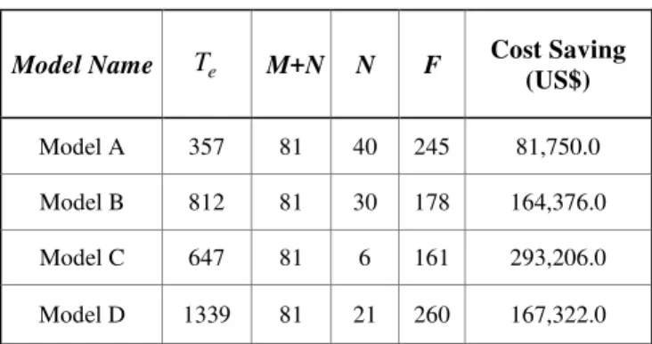
For evaluation purpose, we ran these four models on the test dataset. The test dataset has 1,609,215 instances. Out of the 3506 time-series contained in the test dataset, 81 comprise a validated wheel failure. We applied the proposed evaluation method to estimate the cost saving from these four models. Since we assumed that the operators will act as soon as they receive an alert, we only kept the first alert (prediction of failure) from each time-series. We then extracted the performance parameters N, M, and F by counting the number of time-series for which we did not get any predictions, the number of series for which we did get a prediction followed by an actual failure (true positive), and the number of time-series for which we got a false alert, respectively. To compute, we added the differences between the time of the prediction and the beginning of the target window (i.e., |ptT| ) for each of the M time-series for which the model correctly predicted a failure. In this application, the time unit for the difference |ptT | is “day” and tT is set as 20 days prior to failure. For example,
when the time-to-failure prediction (p) of an alert is 40 days to an actual failure, its difference, |ptT |, is 20 days (
|
|ptT = |-40 – (- 20)| = 20).
The cost information (noted a,b,c, and d in Equations (5) and (6) was provided by an independent expert in the railway industry. These are as follows: a= $2/per day for loss of usage, b=$500/per false alert, c=$5000/per undetected failure and d=$2100/per component replacement. All costs are in US dollars. Using these
values and the results for the performance parameters, we obtained the results shown in Table 2.
Table 2. The results of 4 predictive models on test data
Model Name M+N N F Cost Saving
(US$)
Model A 357 81 40 245 81,750.0 Model B 812 81 30 178 164,376.0 Model C 647 81 6 161 293,206.0 Model D 1339 81 21 260 167,322.0
To compare the evaluation results from different metrics, we also compute accuracy and false alert rate by using generic methods and the scores by using score-based approach by running models on the same test dataset as we computed cost-saving for Table 2. The results are shown in Table 3.
Table 3. The evaluation results from different methods
Model Name Accuracy AUC Score
Cost Saving
(US$)
Model A 75% 0.56 60.5 81,750.0 Model B 89% 0.68 120.5 164,376.0 Model C 93% 0.76 132.8 293,206.0 Model D 86% 0.60 125.0 167,322.0
The case study illustrates the simplicity and usefulness of the cost-based evaluation approach. With this approach, the end user gets a quick understanding of the potential cost savings to be expected from each of the model. Key factors such as timeliness of the alerts and coverage of failures are taken into account, which is not the case with other methods typically used in data mining research. As shown in Table 2, it is obvious that Model C outperformed other models in terms of the cost saving.
From the evaluation results shown in Table 3, it is interesting to note that, for the case study considered, the results obtained from the cast-based method is consistent with the score-based approach. In terms of the AUC and Accuracy results, Model B should be better than Model D. However, the cost-based approach and score-based method
e
show different results. These results support our argument that predictive models deserve specific evaluation methods for its performance evaluation.
6. CONCLUSIONS
In this paper generic methods which are widely used in classifier evaluation are first surveyed. The limitations for existing classifier evaluation, particularly for predictive models evaluation have also been discussed. To address the issues two useful and effectively methods for prognostic model evaluation have been proposed which account for prognostic application specificities. These methods have been used to evaluate the predictive models for several PHM applications such as train wheel prognostics and aircraft component prognostics. In terms of the results obtained from the cast study, it is obvious that the proposed domain-oriented evaluation methods for predictive models are useful and able to provide a direct business value for practitioners.
We believed that more and more feasible and effective domain-oriented approaches will be developed to meet the needs of predictive model evaluation for real-world applications. This is a right way to promote machine learning techniques in solving real-world problems. Domain-oriented approaches may incorporate specificities of domain problems into the performance assessments; therefore, they are helpful and useful in evaluating classifier for applications. At the same time, they are also welcomed by end users because of the feasibility to identify the business values such as cost savings. We strongly argue that a predictive model has to be carefully evaluated not only using generic methods but also domain-oriented approaches before deploying it in PHM applications. Generic methods could help developers in investigating overall performance of a model from the statistical viewpoint at the initial stage of model development. Domain-oriented approaches should be further used to evaluate the usefulness and business value.
ACKNOWLEDGEMENT
This work is supported in part by the National Natural Science Foundation of China (Grant Nos. 61463031).
REFERENCES
Banker R, Chanes A, Cooper W, et al. (1984). Some Models for Estimating Technical and Scale Inefficiencies in Data Envelopment Analysis, Management Science, Vol. 30 No. 9, 1078-1092 Bradley A (1997). The Use of the Area under the ROC
Curve in the Evaluation of Machine Learning Algorithms, Pattern Recognition, Vol. 30, 1145-1159 Caruana R and Niculescu-Mizil A (2006). An Empirical
Comparison of Supervised Learning Algorithms.
Proceedings of the 23rd International Conference on Machine Learning (ICML2006)
Caruana R and Niculescu-Mizil A (2004). Data Mining in Metric Space: An empirical Analysis of Supervised Learning Performance Criteria, Proceedings of the 10th ACM SIGKDD International Conference on Knowledge Discovery and Data Mining (KDD2004), Seattle, Washington, USA, 69-78
Drummond C and Yang C (2008). Reverse-Engineering Costs: How much will a Prognostic Algorithm save?, Proceedings of the 1st International Conference on Prognostics and Health Management. Denver, USA Drummond C and Holte R (2004). What ROC Curve Can’t
Do (and Cost Curve Can), ECAI Workshop on ROC Analysis in Artificial Intelligence
Drummond C and Holte R (2000). Explicitly Representing Expected Cost: An Alternative to ROC Representation, Proceedings of the 6th ACM SIGKDD International Conference on Knowledge Discovery and Data Mining (KDD2000), New York, USA, 155-164
Egan J (1975). Signal Detection Theory and ROC Analysis, New York Academic Press
Fawcett T (2003). ROC Graphs: Notes and Practical Considerations for Data Mining Researchers, Technical report, Intelligent Enterprise Technologies Laboratory, HP
Flach P, (2004). The Many Faces of ROC Analysis in Machine Learning, ICML’04 tutorial, http://www.cs.bris.ac.uk/~flach/ICML04tutorial/ Flach P, (2003). The Geometry of ROC Space:
Understanding Machine Learning Metrics through ROC Isometrics. Proceedings of the 20th International Conference on Machine Learning (ICML03), Washington, DC, USA
Flexer A (1996). Statistical Evaluation of Neural Network Experiments: Minimum Requirement and Current Practice. Proceedings of the 13rd European Meeting on Cybernetics and Systems Research. Austrian Society for Cybernetic Studies, 1005-1008
Giudici P (2003). Applied Data Mining, John Wiley and Sons, New York
Hand D and Till R (2001). A Simple Generalization of the Area Under the ROC Curve for Multiple Class Classification Problems, Machine Learning, Vol.45, 171-186
Huang J and Ling C (2005). Using AUC and Accuracy in Evaluating Learning Algorithms, IEEE Transactions on Knowledge and Data Engineering, Vol. 17, No. 3, 299-310
Japkowicz N. and Shah Mohak (2011). Evaluation of Learning Algorithms, A Classification Perspective, Cambridge University Press
Jardine A., Lin D., and Banjevic D. (2006). A review on machinery diagnostics and prognostics implementing condition-based maintenance. Mechanical Systems and Signal Processing Vol.20, 1483-1510.
Létourneau S, Famili F, et al. (1999). Data Mining for Prediction of Aircraft Component Replacement, IEEE Intelligent Systems Journal, Special Issue on Data Mining. 59-6
Prechelt L (1996). A Quantative Study of Experimental Evaluations of Neural Network Algorithms: Current Research Practice, Neural Networks, Vol. 9
Provost F, Fawcett T and Kohavi R (1998). The case Against Accuracy Estimation for Comparing Induction Algorithms, Proceedings of the 15th International Conference on Machine Learning, 445 – 453
Provost F and Fawcett T (2001). Robust Classification for Imprecise Environment, Machine Learning, Vol.42, No.3, 203-231
Provost F and Fawcett T (1997). Analysis and Visualization of Classifier Performance: Combination under Imprecise Class and Cost Distributions, Proceedings of International Conference on Knowledge Discovery and Data Mining (KDD1997)
Provost F, Fawcett T, and Kohavi R (1998). The case Against Accuracy Estimation for Comparing Induction Algorithms, Proceedings of the 15th International Conference on Machine Learning, 445 – 453
Salzberg S (1997). On Comparing Classifiers: Pitfalls to Avoid and a Recommended Approach. Data Mining & Knowledge Discovery, Vol. 1, 317-328
Saxena A, Sankararaman S, and Goebel K,, (2014). Performance Evaluation for Fleet-based and Unit-based Prognostic Methods, European Conference of the Prognostics and Health Management Society
Saxena A, Celaya J., Saha B, Saha S, and Goebel K. (2009). On Applying the Prognostic Performance Metrics, Proceedings of International Conference on Prognostics and Health Management
Schwabacher M and Goebel K (2007). A Survey of Artificial Intelligence for Prognostics, The 2007 AAAI Fall Symposium, Arlington, Virginal, USA
Srinivasan A (1999). Note on the location of optimal classifiers in n-dimensional ROC space. Technical Report PRG-TR-2-99, Oxford University Computing Laboratory
Swets J, Dwaes R, et al. (2000). Psychological Science Can Improve Diagnostic decisions, Psychological Science in the Public Interest, Vol. 1, 1-26
Yang C and Létourneau S (2007). Model Evaluation for Prognostics: Estimating Cost Saving for the End Users, The Proceedings of the 6th International Conference on Machine Learning and Applications (ICMLA 2007), Cincinnati, OH, USA
Yang C and Létourneau S (2005). Learning to Predict Train Wheel Failures, Proceedings of the 11th ACM SIGKDD International Conference on Knowledge Discovery and Data Mining (KDD2005), 516-525
Zheng Z, Padmanabhan B, et al. (2004). A DEA Approach for Model Combination, Proceedings of the 10th ACM SIGKDD International Conference on Knowledge
Discovery and Data Mining (KDD2004), Seattle, Washington, USA, 755-758
BIOGRAPHIES
Chunsheng Yang is a Senior Research Officer at the
National Research Council Canada. He is interested in data mining, machine learning, prognostic health management(PHM), reasoning technologies such as case-based reasoning, rule-case-based reasoning and hybrid reasoning, multi-agent systems, and distributed computing. He received an Hons. B.Sc. in Electronic Engineering from Harbin Engineering University, China, an M.Sc. in computer science from Shanghai Jiao Tong University, China, and a Ph.D. from National Hiroshima University, Japan. He worked with Fujitsu Inc., Japan, as a Senior Engineer and engaged on the development of ATM Network Management Systems. He was an Assistant Professor at Shanghai Jiao Tong University from 1986 to 1990 working on Hypercube Distributed Computer Systems. He was a Program Co-Chair for the 17th International Conference on Industry and Engineering Applications of Artificial Intelligence and Expert Systems. Dr. Yang is a guest editor for the International Journal of Applied Intelligence. He has served Program Committees for many conferences and institutions, and has been a reviewer for many conferences, journals, and organizations, including Applied Intelligence, NSERC, IEEE Trans., ACM KDD, PAKDD, AAMAS, IEA/AIE. Dr. Yang is a Senior IEEE member.
Yanni Zou is an Assistant Professor with Jiujiang
University, Jiangxi, China. She is also a Ph.D. Candidate at School of Information Technology, Nanchang University. She is interested in image processing, process control, robotics, intelligent systems, and machine learning. She received an Hons. B.Sc. in Electronic Engineering from Nanchang University China, an M.Sc. in System Engineering, Anhui University of Science and Technology, Anhui, China.
Jie Liu is currently an Assistant Professor in the
Department of Mechanical & Aerospace Engineering at Carleton University, Ottawa, Canada. He received his B.Eng. in Electronics and Precision Engineering from Tianjin University, China, his M.Sc. in Control Engineering from Lakehead University, Canada, and his Ph.D. in Mechanical Engineering from the University of Waterloo, Canada. He is leading research efforts in the areas of prognostics and health management, intelligent mechatronic systems, power generation and storage. He has published over 25 papers in peer-reviewed journals. He is also a registered professional engineer in Ontario, Canada.
Kyle R Mulligan obtained his Bachelor’s degree in
Systems and Computer Engineering at Carleton University in Ottawa in 2007. He then continued to obtain his Master’s degree in Biomedical Engineering in 2009 at Carleton
University. In 2014 he completed a Doctorate degree in Mechanical Engineering at the Université de Sherbrooke with a specialization in data-driven prognostics for assessing structural failures. He is an active volunteer at local high schools to promote the awareness and importance of Engineering in today’s society. His research interests include: medical imaging techniques, biomechanics, nanorobotics, and structural/prognostic health management.