Sentiment analysis of short informal texts

Publisher’s version / Version de l'éditeur:

Journal of Artifcial Intelligence Research, 50, pp. 723-762, 2014-08-01

READ THESE TERMS AND CONDITIONS CAREFULLY BEFORE USING THIS WEBSITE. https://nrc-publications.canada.ca/eng/copyright

Vous avez des questions? Nous pouvons vous aider. Pour communiquer directement avec un auteur, consultez la

première page de la revue dans laquelle son article a été publié afin de trouver ses coordonnées. Si vous n’arrivez

Questions? Contact the NRC Publications Archive team at

[email protected]. If you wish to email the authors directly, please see the first page of the publication for their contact information.

This publication could be one of several versions: author’s original, accepted manuscript or the publisher’s version. / La version de cette publication peut être l’une des suivantes : la version prépublication de l’auteur, la version acceptée du manuscrit ou la version de l’éditeur.

For the publisher’s version, please access the DOI link below./ Pour consulter la version de l’éditeur, utilisez le lien DOI ci-dessous.

https://doi.org/10.1613/jair.4272

Access and use of this website and the material on it are subject to the Terms and Conditions set forth at

Sentiment analysis of short informal texts

Kiritchenko, Svetlana; Zhu, Xiaodan; Mohammad, Saif M.

https://publications-cnrc.canada.ca/fra/droits

L’accès à ce site Web et l’utilisation de son contenu sont assujettis aux conditions présentées dans le site LISEZ CES CONDITIONS ATTENTIVEMENT AVANT D’UTILISER CE SITE WEB.

NRC Publications Record / Notice d'Archives des publications de CNRC:

Sentiment Analysis of Short Informal Texts

Svetlana Kiritchenko [email protected]

Xiaodan Zhu [email protected]

Saif M. Mohammad [email protected]

National Research Council Canada 1200 Montreal Rd., Ottawa, ON, Canada

Abstract

We describe a state-of-the-art sentiment analysis system that detects (a) the sentiment of short informal textual messages such as tweets and SMS (message-level task) and (b) the sentiment of a word or a phrase within a message (term-level task). The system is based on a supervised statistical text classification approach leveraging a variety of surface-form, semantic, and sentiment features. The sentiment features are primarily derived from novel high-coverage tweet-specific sentiment lexicons. These lexicons are automatically generated from tweets with sentiment-word hashtags and from tweets with emoticons. To adequately capture the sentiment of words in negated contexts, a separate sentiment lexicon is generated for negated words.

The system ranked first in the SemEval-2013 shared task ‘Sentiment Analysis in Twit-ter’ (Task 2), obtaining an F-score of 69.02 in the message-level task and 88.93 in the term-level task. Post-competition improvements boost the performance to an F-score of 70.45 (message-level task) and 89.50 (term-level task). The system also obtains state-of-the-art performance on two additional datasets: the SemEval-2013 SMS test set and a corpus of movie review excerpts. The ablation experiments demonstrate that the use of the automatically generated lexicons results in performance gains of up to 6.5 absolute percentage points.

1. Introduction

Sentiment Analysis involves determining the evaluative nature of a piece of text. For ex-ample, a product review can express a positive, negative, or neutral sentiment (or polarity). Automatically identifying sentiment expressed in text has a number of applications, in-cluding tracking sentiment towards products, movies, politicians, etc., improving customer relation models, detecting happiness and well-being, and improving automatic dialogue sys-tems. Over the past decade, there has been a substantial growth in the use of microblogging services such as Twitter and access to mobile phones world-wide. Thus, there is tremendous interest in sentiment analysis of short informal texts, such as tweets and SMS messages, across a variety of domains (e.g., commerce, health, military intelligence, and disaster man-agement).

Short informal textual messages bring in new challenges to sentiment analysis. They are limited in length, usually spanning one sentence or less. They tend to have many misspellings, slang terms, and shortened forms of words. They also have special markers such as hashtags that are used to facilitate search, but can also indicate a topic or sentiment. This paper describes a state-of-the-art sentiment analysis system addressing two tasks: (a) detecting the sentiment of short informal textual messages (message-level task) and

(b) detecting the sentiment of a word or a phrase within a message (term-level task). The system is based on a supervised statistical text classification approach leveraging a variety of surface-form, semantic, and sentiment features. Given only limited amounts of training data, statistical sentiment analysis systems often benefit from the use of manually or automatically built sentiment lexicons. Sentiment lexicons are lists of words (and phrases) with prior associations to positive and negative sentiments. Some lexicons can additionally provide a sentiment score for a term to indicate its strength of evaluative intensity. Higher scores indicate greater intensity. For example, an entry great (positive, 1.2) states that the word great has positive polarity with the sentiment score of 1.2. An entry acceptable (positive, 0.1) specifies that the word acceptable has positive polarity and its intensity is lower than that of the word great.

In our sentiment analysis system, we utilize three freely available, manually created, general-purpose sentiment lexicons. In addition, we generated two high-coverage tweet-specific sentiment lexicons from about 2.5 million tweets using sentiment markers within them. These lexicons automatically capture many peculiarities of the social media language such as common intentional and unintentional misspellings (e.g., gr8, lovin, coul, holys**t), elongations (e.g., yesssss, mmmmmmm, uugghh), and abbreviations (e.g., lmao, wtf ). They also include words that are not usually considered to be expressing sentiment, but that are often associated with positive/negative feelings (e.g., party, birthday, homework ).

Sentiment lexicons provide knowledge on prior polarity (positive, negative, or neutral) of a word, i.e., its polarity in most contexts. However, in a particular context this prior polarity can change. One such obvious contextual sentiment modifier is negation. In a negated context, many words change their polarity or at least the evaluative intensity. For example, the word good is often used to express positive attitude whereas the phrase not good is clearly negative. A conventional way of addressing negation in sentiment analysis is to reverse the polarity of a word, i.e. change a word’s sentiment score from s to −s (Kennedy & Inkpen, 2005; Choi & Cardie, 2008). However, several studies have pointed out the inadequacy of this solution (Kennedy & Inkpen, 2006; Taboada, Brooke, Tofiloski, Voll, & Stede, 2011). We will show through experiments in Section 4.3 that many positive terms, though not all, tend to reverse their polarity when negated, whereas most negative terms remain negative and only change their evaluative intensity. For example, the word terrible conveys a strong negative sentiment whereas the phrase wasn’t terrible is mildly negative. Also, the degree of the intensity shift varies from term to term for both posi-tive and negaposi-tive terms. To adequately capture the effects of negation on different terms, we propose a corpus-based statistical approach to estimate sentiment scores of individual terms in the presence of negation. We build two lexicons: one for words in negated contexts (Negated Context Lexicon) and one for words in affirmative (non-negated) contexts (Affir-mative Context Lexicon). Each word (or phrase) now has two scores, one in the Negated Context Lexicon and one in the Affirmative Context Lexicon. When analyzing the sen-timent of a textual message, we use scores from the Negated Context Lexicon for words appearing in a negated context and scores from the Affirmative Context Lexicon for words appearing in an affirmative context.

Experiments are carried out to asses both, the performance of the overall sentiment analysis system as well as the quality and value of the automatically created tweet-specific lexicons. In the intrinsic evaluation of the lexicons, their entries are compared with the

entries of the manually created lexicons. Also, human annotators were asked to rank a subset of lexicon entries by the degree of their association with positive or negative sentiment and this ranking is compared with the ranking produced by an automatic lexicon. In both experiments we observe high agreement between the automatic and manual sentiment annotations.

The extrinsic evaluation is performed on two tasks: unsupervised and supervised sen-timent analysis. On the supervised task, we assess the performance of the full sensen-timent analysis system and examine the impact of the features derived from the automatic lexicons on the overall performance. As a testbed, we use the datasets provided for the SemEval-2013 competition on Sentiment Analysis in Twitter (Wilson, Kozareva, Nakov, Rosenthal,

Stoyanov, & Ritter, 2013).1 There were datasets provided for two tasks, message-level task

and term-level task, and two domains, tweets and SMS. However, the training data were available only for tweets. Among 77 submissions from 44 teams, our system placed first in the competition in both tasks on the tweet test set, obtaining a macro-averaged F-score of 69.02 in the message-level task and 88.93 in the term-level task. Post-competition im-provements to the system boost the performance to an F-score of 70.45 (message-level task) and 89.50 (term-level task). We also applied our classifier on the SMS test set without any further tuning. The classifier obtained the first position in identifying sentiment of SMS messages (F-score of 68.46) and the second position in detecting the sentiment of terms within SMS messages (F-score of 88.00; only 0.39 points behind the first-ranked sys-tem). With post-competition improvements, the system achieves an F-score of 69.77 in the message-level task and an F-score of 88.20 in the term-level task on that test set.

In addition, we evaluate the performance of our sentiment analysis system on the domain of movie review excerpts (message-level task only). The system is re-trained on a collection of about 7,800 positive and negative sentences extracted from movie reviews. When applied on the test set of unseen sentences, the system is able to correctly classify 85.5% of the test set. This result exceeds the best result obtained on this dataset by a recursive deep learning approach that requires access to sentiment labels of all syntactic phrases in the training-data sentences (Socher, Perelygin, Wu, Chuang, Manning, Ng, & Potts, 2013). For the message-level task, we do not make use of sentiment labels of phrases in the training data, as that is often unavailable in real-world applications.

The ablation experiments reveal that the automatically built lexicons gave our system the competitive advantage in SemEval-2013. The use of the new lexicons results in gains of up to 6.5 percentage points over the gains obtained through the use of other features. Furthermore, we show that the lexicons built specifically for negated contexts better model negation than the reversing polarity approach.

The main contributions of this paper are three-fold. First, we present a sentiment analysis system that achieves state-of-the-art performance on three domains: tweets, SMS, and movie review excerpts. The system can be replicated using freely available resources. Second, we describe the process of creating the automatic, tweet-specific lexicons and demonstrate their superior predictive power over several manually and automatically cre-ated general-purpose lexicons. Third, we analyze the impact of negation on sentiment and propose an empirical method to estimate the sentiment of words in negated contexts by

1. SemEval is an international forum for natural-language shared tasks. The competition we refer to is SemEval-2013 Task 2 (http://www.cs.york.ac.uk/semeval-2013/task2).

creating a separate sentiment lexicon for negated words. All automatic lexicons described

in the paper are made available to the research community.2

The paper is organized as follows. We begin with a description of related work in Sec-tion 2. Next, we describe the sentiment analysis task and the data used in this research (Section 3). Section 4 presents the sentiment lexicons used in our system: existing manually created, general-purpose lexicons (Section 4.1) and our automatic, tweet-specific lexicons (Section 4.2). The lexicons built for affirmative and negated contexts are described in Sec-tion 4.3. The detailed descripSec-tion of our supervised sentiment analysis system, including the classification method and the feature sets, is presented in Section 5. Section 6 provides the results of the evaluation experiments. First, we compare the automatically created lexi-cons with human annotations derived from the manual lexilexi-cons as well as collected through

Amazon’s Mechanical Turk service3 _{(Section 6.1). Next, we evaluate the new lexicons on}

the extrinsic task of unsupervised sentiment analysis (Section 6.2.1). The purpose of these experiments is to compare the predictive capacity of the individual lexicons without in-fluence of other factors. Then, in Section 6.2.2 we assess the performance of the entire supervised sentiment analysis system and examine the contribution of the features derived from our lexicons to the overall performance. Finally, we conclude and present directions for future work in Section 7.

2. Related Work

Over the last decade, there has been an explosion of work exploring various aspects of sentiment analysis: detecting subjective and objective sentences; classifying sentences as positive, negative, or neutral; detecting the person expressing the sentiment and the target of the sentiment; detecting emotions such as joy, fear, and anger; visualizing sentiment in text; and applying sentiment analysis in health, commerce, and disaster management. Surveys by Pang and Lee (2008) and Liu and Zhang (2012) give a summary of many of these approaches.

Sentiment analysis systems have been applied to many different kinds of texts including customer reviews, news paper headlines (Bellegarda, 2010), novels (Boucouvalas, 2002; John, Boucouvalas, & Xu, 2006; Francisco & Gerv´as, 2006; Mohammad & Yang, 2011), emails (Liu, Lieberman, & Selker, 2003; Mohammad & Yang, 2011), blogs (Neviarouskaya, Prendinger, & Ishizuka, 2011; Genereux & Evans, 2006; Mihalcea & Liu, 2006), and tweets (Mohammad, 2012). Often these systems have to cater to the specific needs of the text such as formality versus informality, length of utterances, etc. Sentiment analysis systems developed specifically for tweets include those by Pak and Paroubek (2010), Agarwal, Xie, Vovsha, Rambow, and Passonneau (2011), Thelwall, Buckley, and Paltoglou (2011), Brody and Diakopoulos (2011), Aisopos, Papadakis, Tserpes, and Varvarigou (2012), Bakliwal,

Arora, Madhappan, Kapre, Singh, and Varma (2012). A recent survey by Mart´ınez-C´amara,

Mart´ın-Valdivia, Ure˜nal´opez, and Montejor´aez (2012) provides an overview of the research

on sentiment analysis of tweets.

Several manually created sentiment resources have been successfully applied in sentiment analysis. The General Inquirer has sentiment labels for about 3,600 terms (Stone, Dunphy,

2. www.purl.com/net/sentimentoftweets 3. https://www.mturk.com/mturk/welcome

Smith, Ogilvie, & associates, 1966). Hu and Liu (2004) manually labeled about 6,800 words and used them for detecting sentiment of customer reviews. The MPQA Subjectivity Lexicon, which draws from the General Inquirer and other sources, has sentiment labels for about 8,000 words (Wilson, Wiebe, & Hoffmann, 2005). The NRC Emotion Lexicon has sentiment and emotion labels for about 14,000 words (Mohammad & Turney, 2010). These labels were compiled through Mechanical Turk annotations.

Semi-supervised and automatic methods have also been proposed to detect the polarity of words. Hatzivassiloglou and McKeown (1997) proposed an algorithm to determine the polarity of adjectives. SentiWordNet (SWN) was created using supervised classifiers as well as manual annotation (Esuli & Sebastiani, 2006). Turney and Littman (2003) proposed a minimally supervised algorithm to calculate the polarity of a word by determining if its tendency to co-occur with a small set of positive seed words is greater than its tendency to co-occur with a small set of negative seed words. Mohammad, Dunne, and Dorr (2009) automatically generated a sentiment lexicon of more than 60,000 words from a thesaurus. We use several of these lexicons in our system. In addition, we create two new sentiment lexicons from tweets using hashtags and emoticons. In Section 6, we show that these tweet-specific lexicons have a higher coverage and a better predictive power than the lexicons mentioned earlier.

Since manual annotation of data is costly, distant supervision techniques have been ac-tively applied in the domain of short informal texts. User-provided indications of emotional content, such as emoticons, emoji, and hashtags, have been used as noisy sentiment labels. For example, Go, Bhayani, and Huang (2009) use tweets with emoticons as labeled data for supervised training. Emoticons such as :) are considered positive labels of the tweets and emoticons such as :( are used as negative labels. Davidov, Tsur, and Rappoport (2010) and Kouloumpis, Wilson, and Moore (2011) use certain seed hashtag words such as #cute and #sucks as labels of positive and negative sentiment. Mohammad (2012) developed a classi-fier to detect emotions using tweets with emotion word hashtags (e.g., #anger, #surprise) as labeled data.

In our system too, we make use of the emoticons and hashtag words as signals of positive and negative sentiment. We collected 775,000 sentiment-word hashtagged tweets and used 1.6 million emoticon tweets collected by Go et al. (2009). However, unlike previous research, we generate sentiment lexicons from these datasets and use them (along with a relatively small hand-labeled training dataset) to train a supervised classifier. This approach has the following benefits. First, it allows us to incorporate large amounts of noisily labeled data quickly and efficiently. Second, the classification system is robust to the introduced noise because the noisy data are incorporated not directly as training instances but indirectly as features. Third, the generated sentiment lexicons can be easily distributed among the research community and employed in other applications and on other domains (Kiritchenko, Zhu, Cherry, & Mohammad, 2014).

Negation plays an important role in determining sentiment. Automatic negation han-dling involves identifying a negation word such as not, determining the scope of negation (which words are affected by the negation word), and finally appropriately capturing the impact of the negation. (See work by Jia, Yu, and Meng (2009), Wiegand, Balahur, Roth, Klakow, and Montoyo (2010), Lapponi, Read, and Ovrelid (2012) for detailed analyses of negation handling.) Traditionally, the negation word is determined from a small

hand-crafted list (Taboada et al., 2011). The scope of negation is often assumed to begin from the word following the negation word until the next punctuation mark or the end of the sentence (Polanyi & Zaenen, 2004; Kennedy & Inkpen, 2005). More sophisticated methods to detect the scope of negation through semantic parsing have also been proposed (Li, Zhou, Wang, & Zhu, 2010).

A common way to capture the impact of negation is to reverse the polarities of the sentiment words in the scope of negation. Taboada et al. (2011) proposed to shift the sentiment score of a term in a negated context towards the opposite polarity by a fixed amount. However, in their experiments the shift-score model did not agree with human judgment in many cases, especially for negated negative terms. More complex approaches, such as recursive deep models, address negation through semantic composition (Socher, Huval, Manning, & Ng, 2012; Socher et al., 2013). The recursive deep models work in a bottom-top fashion over a parse-tree structure of a sentence to infer the sentiment label of the sentence as a composition of the sentiment expressed by its constituting parts: words and phrases. These models do not require any hand-crafted features or semantic knowledge, such as a list of negation words. However, they are computationally intensive and need substantial additional annotations (word and phrase-level sentiment labeling) to produce competitive results (Socher et al., 2013). In this paper, we propose a simple corpus-based statistical method to estimate the sentiment scores of negated words. As will be shown in Section 6.2.2, this simple method is able to achieve the same level of accuracy as the recursive deep learning approach. Additionally, we analyze the impact of negation on sentiment scores of common sentiment terms.

To promote research in sentiment analysis of short informal texts and to establish a common ground for comparison of different approaches, an international competition was organized by the Conference on Semantic Evaluation Exercises (SemEval-2013) (Wilson et al., 2013). The organizers created and shared tweets for training, development, and testing. They also provided a second test set consisting of SMS messages. The purpose of having this out-of-domain test set was to assess the ability of the systems trained on tweets to generalize to other types of short informal texts. The competition attracted 44 teams; there were 48 submissions from 34 teams in the message-level task and 29 submissions from 23 teams in the term-level task. Most participants (including the top 3 systems in each task) chose a supervised machine learning approach exploiting a variety of features derived from ngrams, stems, punctuation, POS tags, and Twitter-specific encodings (e.g., emoticons, hashtags, abbreviations). Only one of the top-performing systems was entirely rule-based with hand-written rules (Reckman, Baird, Crawford, Crowell, Micciulla, Sethi, & Veress, 2013). Twitter-specific pre-processing (e.g., tokenization, normalization) as well as negation handling were commonly applied. Almost all systems benefited from sentiment lexicons: MPQA Subjectivity Lexicon, SentiWordNet, and others. Existing, low-coverage lexicons were sometimes extended with distributionally similar words (Proisl, Greiner, Evert, & Kabashi, 2013) or sentiment-associated words collected from noisily labeled data (Becker, Erhart, Skiba, & Matula, 2013). Those extended lexicons, however, were still an order of magnitude smaller than the tweet-specific lexicons we created. For the full results of the competition and further details we refer the reader to Wilson et al. (2013).

Some research approaches sentiment analysis as a two-tier problem: first a piece of text is marked as either objective or subjective, and then only the subjective text is assessed

to determine whether it is positive, negative, or neutral (Wiebe, Wilson, & Cardie, 2005; Choi & Cardie, 2010; Johansson & Moschitti, 2013; Yang & Cardie, 2013). However, this can lead to a propagation of errors (for example, the system may mark a subjective text as objective). Further, one can argue that even objective statements can express sentiment (for example, “the sales of Blackberries are 0.002% of what they used to be 5 years back”). We model sentiment directly as a three-class problem: positive, negative, or neutral.

Also, this paper focuses on sentiment analysis alone and does not consider the task of associating the sentiment with its targets. There has been interesting work studying the latter problem (e.g., Jiang, Yu, Zhou, Liu, & Zhao, 2011; Sauper & Barzilay, 2013). In (Kiritchenko et al., 2014) we show how our approach can be adapted to identify the sentiment for a specified target. The system ranked first in the SemEval-2014 shared task ‘Aspect Based Sentiment Analysis’.

3. Task and Data Description

In this work, we follow the definition of the task and use the data provided for the SemEval-2013 competition: Sentiment Analysis in Twitter (Wilson et al., SemEval-2013). This competition had two tasks: a level task and a term-level task. The objective of the message-level task is to detect whether the whole message conveys a positive, negative, or neutral sentiment. The objective of the term-level task is to detect whether a given target term (a single word or a multi-word expression) conveys a positive, negative, or neutral sentiment in the context of a message. Note that the same term may express different sentiments in different contexts. For example, the word unpredictable expresses positive sentiment in sentence “The movie has an unpredictable ending”; whereas, it expresses negative sentiment in sentence “The car has unpredictable steering”.

Two test sets – one with tweets and one with SMS messages – were provided to the participants for each task. Training and development data were available only for tweets. Here we briefly describe how the data were collected and annotated (for more details see the task description paper (Wilson et al., 2013)). Tweets were collected through the public streaming Twitter API during a period of one year: from January 2012 to January 2013. To reduce the data skew towards the neutral class, messages that did not contain any polarity word listed in SentiWordNet 3.0 were discarded. The remaining messages were annotated for

sentiment through Mechanical Turk.4 _{Each annotator had to mark the positive, negative,}

and neutral parts of a message as well as to provide the overall polarity label for the message. Later, the annotations were combined through intersection for the term-level task and by majority voting for the message-level task. The details on data collection and annotation were released to the participants after the competition.

The data characteristics for both tasks are shown in Table 1. The training set was distributed through tweet ids and a download script. However, not all tweets were accessible. For example, a Twitter user could have deleted her messages, and thus these messages would not be available. Table 1 shows the number of the training examples we were able to download. The development and test sets were provided in full by FTP.

Table 1: Data statistics for the SemEval-2013 training set, development set and two testing sets. “# of tokens per mess.” denotes the average number of tokens per message in the dataset. “Vocab. size” represents the number of unique tokens excluding punctuation and numerals.

Number of instances # tokens Vocab. Dataset Positive Negative Neutral Total per mess. size Message-level task:

Training set 3,045 (37%) 1,209 (15%) 4,004 (48%) 8,258 22.09 21,848 Development set 575 (35%) 340 (20%) 739 (45%) 1,654 22.19 6,543 Tweet test set 1,572 (41%) 601 (16%) 1,640 (43%) 3,813 22.15 12,977 SMS test set 492 (23%) 394 (19%) 1,208 (58%) 2,094 18.05 3,513 Term-level task:

Training set 4,831 (62%) 2,540 (33%) 385 (5%) 7,756 22.55 15,238 Development set 648 (57%) 430 (38%) 57 (5%) 1,135 22.93 3,909 Tweet test set 2,734 (62%) 1,541 (35%) 160 (3%) 4,435 22.63 10,383 SMS test set 1,071 (46%) 1,104 (47%) 159 (7%) 2,334 19.95 2,979

The tweets are comprised of regular English-language words as well as Twitter-specific

terms, such as emoticons, URLs, and creative spellings. Using WordNet 3.05 (147,278

word types) supplemented with a large list of stop words (571 words)6 _{as a repository of}

English-language words, we found that about 45% of the vocabulary in the tweet datasets are out-of-dictionary terms. These out-of-dictionary terms fall into different categories, e.g., named entities (names of people, places, companies, etc.) not found in WordNet, hashtags, user mentions, etc. We use the Carnegie Mellon University (CMU) Twitter NLP tool to automatically identify the categories. The tool was shown to achieve 89% tagging accuracy on tweet data (Gimpel, Schneider, O’Connor, Das, Mills, Eisenstein, Heilman, Yogatama, Flanigan, & Smith, 2011). Table 2 shows the distribution of the out-of-dictionary terms by

category.7 One can observe that most of the out-of-dictionary terms are named entities as

well as user mentions, URLs, and hashtags. There is also a moderate amount of creatively spelled regular English words and slang words used as nouns, verbs, and adjectives. In the SMS test set, out-of-dictionary terms constitute a smaller proportion of the vocabulary, about 25%. These are mostly named entities, interjections, creative spellings, and slang.

The SemEval-2013 training and development data are used to train our supervised sen-timent analysis system presented in Section 5. The performance of the system is evaluated on both test sets, tweets and SMS (Section 6.2.2). The test data are also used in the experiments on comparing the performance of sentiment lexicons in unsupervised settings (Section 6.2.1).

5. http://wordnet.princeton.edu

6. The SMART stopword list built by Gerard Salton and Chris Buckley for the SMART information retrieval system at Cornell University (http://www.lextek.com/manuals/onix/stopwords2.html) is used.

7. The percentages in the columns do not sum up to 100% because some terms can be used in multiple categories (e.g., as a noun and a verb).

Table 2: The distribution of the out-of-dictionary tokens by category for the SemEval-2013 tweet and SMS test sets.

Category of tokens Tweet test set SMS test set named entities 31.84% 32.63% user mentions 21.23% 0.11% URLs 16.92% 0.84% hashtags 10.94% 0% interjections 2.56% 10.32% emoticons 1.40% 1.89% nouns 8.52% 25.47% verbs 3.05% 18.95% adjectives 1.43% 4.84% adverbs 0.70% 6.21% others 4.00% 15.69%

In addition to the SemEval-2013 datasets, we evaluate the system on a dataset of movie review excerpts (Socher et al., 2013). The task is to predict the sentiment label (positive or negative) of a given sentence, extracted from a longer movie review (message-level task). The dataset is comprised of 4,963 positive and 4,650 negative sentences split into the train-ing (6,920 sentences), development (872 sentences), and test (1,821 sentences) sets. Since detailed phrase-level annotations are not available for most real-world applications, we use only sentence-level annotations and ignore the phrase-level annotations and the parse-tree structures of the sentences provided with the data. We train our sentiment analysis system on the training and development subsets and evaluate its performance on the test subset. The results of these experiments are reported in Section 6.2.2.

4. Sentiment Lexicons Used by Our System

4.1 Existing, General-Purpose, Manually Created Sentiment Lexicons

Most of the lexicons that were created by manual annotation tend to be domain free and include a few thousand terms. The lexicons that we use include the NRC Emotion Lexicon (Mohammad & Turney, 2010), Bing Liu’s Lexicon (Hu & Liu, 2004), and the MPQA Sub-jectivity Lexicon (Wilson et al., 2005). The NRC Emotion Lexicon is comprised of frequent English nouns, verbs, adjectives, and adverbs annotated for eight emotions (joy, sadness, anger, fear, disgust, surprise, trust, and anticipation) as well as for positive and negative sentiment. Bing Liu’s Lexicon provides a list of positive and negative words manually ex-tracted from customer reviews. The MPQA Subjectivity Lexicon contains words marked with their prior polarity (positive or negative) and a discrete strength of evaluative intensity (strong or weak). Entities in these lexicons do not come with a real-valued score indicating the fine-grained evaluative intensity.

4.2 New, Tweet-Specific, Automatically Generated Sentiment Lexicons 4.2.1 Hashtag Sentiment Lexicon

Certain words in tweets are specially marked with a hashtag (#) and can indicate the topic or sentiment. Mohammad (2012) showed that hashtagged emotion words such as #joy, #sad, #angry, and #surprised are good indicators that the tweet as a whole (even without the hashtagged emotion word) is expressing the same emotion. We adapted that idea to create a large corpus of positive and negative tweets. From this corpus we then automatically generated a high-coverage, tweet-specific sentiment lexicon as described below.

We polled the Twitter API every four hours from April to December 2012 in search of tweets with either a positive-word hashtag or a negative-word hashtag. A collection of 77 seed words closely associated with positive and negative sentiment such as #good, #excellent, #bad, and #terrible were used (30 positive and 47 negative). These terms were

chosen from entries for positive and negative in Roget’s Thesaurus8. About 2 million tweets

were collected in total. We used the metadata tag “iso language code” to identify English tweets. Since this tag is not always reliable, we additionally discarded tweets that did not

have at least two valid English content words from Roget’s Thesaurus.9 This step also

helped discard very short tweets and tweets with a large proportion of misspelled words. A set of 775,000 remaining tweets, which we refer to as Hashtag Sentiment Corpus, was used to generate a large word–sentiment association lexicon. A tweet was considered positive if it had one of the 30 positive hashtagged seed words, and negative if it had one of the 47 negative hashtagged seed words. The sentiment score for a term w was calculated from these pseudo-labeled tweets as shown below:

Sentiment Score (w) = PMI (w , positive) − PMI (w , negative) (1)

PMI stands for pointwise mutual information: PMI (w , positive) = log2

freq (w , positive) ∗ N

freq (w ) ∗ freq (positive) (2)

where freq (w, positive) is the number of times a term w occurs in positive tweets, freq (w) is the total frequency of term w in the corpus, freq (positive) is the total number of tokens in positive tweets, and N is the total number of tokens in the corpus. PMI (w, negative) is calculated in a similar way. Thus, equation 1 is simplified to:

Sentiment Score (w) = log2

freq (w , positive) ∗ freq (negative)

freq (w , negative) ∗ freq (positive) (3)

Since PMI is known to be a poor estimator of association for low-frequency events, we ignore terms that occurred less than five times in each (positive and negative) group of tweets.10

8. http://www.gutenberg.org/ebooks/10681

9. Any word in the thesaurus was considered a content word with the exception of the words from the SMART stopword list.

10. The same threshold of five occurrences in at least one class (positive or negative) is applied for all automatic tweet-specific lexicons discussed in this paper. There is no thresholding on the sentiment score.

A positive sentiment score indicates a greater overall association with positive sentiment, whereas a negative score indicates a greater association with negative sentiment. The magnitude is indicative of the degree of association. Note that there exist numerous other methods to estimate the degree of association of a term with a category (e.g., cross entropy, Chi-squared, and information gain). We have chosen PMI because it is simple and robust and has been successfully applied in a number of NLP tasks (Turney, 2001; Turney & Littman, 2003).

The final lexicon, which we will refer to as Hashtag Sentiment Base Lexicon (HS Base) has entries for 39,413 unigrams and 178,851 bigrams. Entries were also generated for unigram–unigram, unigram–bigram, and bigram–bigram pairs that were not necessarily contiguous in the tweets corpus. Pairs where at least one of the terms is punctuation (e.g., “,”, “?”, “.”), a user mention, a URL, or a function word (e.g., “a”, “the”, “and”) were removed. The lexicon has entries for 308,808 non-contiguous pairs.

4.2.2 Sentiment140 Lexicon

The Sentiment140 Corpus (Go et al., 2009) is a collection of 1.6 million tweets that contain emoticons. The tweets are labeled positive or negative according to the emoticon. We generated the Sentiment140 Base Lexicon (S140 Base) from this corpus in the same manner as described above for the hashtagged tweets using Equation 1. This lexicon has entries for 65,361 unigrams, 266,510 bigrams, and 480,010 non-contiguous pairs. In the following section, we further build on the proposed approach to create separate lexicons for terms in affirmative contexts and for terms in negated contexts.

4.3 Affirmative Context and Negated Context Lexicons

A word in a negated context has a different evaluative nature than the same word in an affirmative (non-negated) context. This difference may include the change in the polarity category (positive becomes negative or vice versa), the evaluative intensity, or both. For example, highly positive words (e.g., great) when negated tend to experience both, polarity change and intensity decrease, forming mildly negative phrases (e.g., not great). On the other hand, many strong negative words (e.g., terrible) when negated keep their negative polarity and just shift their intensity. The conventional approach of reversing polarity is not able to handle these cases properly.

We propose an empirical method to determine the sentiment of words in the presence of negation. We create separate lexicons for affirmative and negated contexts. In this way, two sentiment scores for each term w are computed: one for affirmative contexts and another for negated contexts. The lexicons are created as follows. The Hashtag Sentiment Corpus is split into two parts: Affirmative Context Corpus and Negated Context Corpus. Following the work by Pang, Lee, and Vaithyanathan (2002), we define a negated context as a segment of a tweet that starts with a negation word (e.g., no, shouldn’t) and ends with one of the punctuation marks: ‘,’, ‘.’, ‘:’, ‘;’, ‘!’, ‘?’. The list of negation words was adopted from

Christopher Potts’ sentiment tutorial.11 _{Thus, part of a tweet that is marked as negated}

is included into the Negated Context Corpus while the rest of the tweet becomes part of the Affirmative Context Corpus. The sentiment label for the tweet is kept unchanged

Table 3: Example sentiment scores from the Sentiment140 Base, Affirmative Context (AffLex) and Negated Context (NegLex) Lexicons.

Term Sentiment140 Lexicons Base AffLex NegLex Positive terms great 1.177 1.273 -0.367 beautiful 1.049 1.112 0.217 nice 0.974 1.149 -0.912 good 0.825 1.167 -1.414 honest 0.391 0.431 -0.123 Negative terms terrible -1.766 -1.850 -0.890 shame -1.457 -1.548 -0.722 bad -1.297 -1.674 0.021 ugly -0.899 -0.964 -0.772 negative -0.090 -0.261 0.389

in both corpora. Then, we generate the Affirmative Context Lexicon (HS AffLex) from the Affirmative Context Corpus and the Negated Context Lexicon (HS NegLex) from the Negated Context Corpus using the technique described in Section 4.2. We will refer to

the sentiment score calculated from the Affirmative Context Corpus as scoreAffLex(w ) and

the score calculated from the Negated Context Corpus as scoreNegLex(w ). Similarly, the

Sentiment140 Affirmative Context Lexicon (S140 AffLex) and the Sentiment140 Negated Context Lexicon (S140 NegLex) are built from the Affirmative Context and the Negated Context parts of the Sentiment140 tweet corpus. To employ these lexicons on a separate dataset, we apply the same technique to split each message into affirmative and negated contexts and then match words in affirmative contexts against the Affirmative Context Lexicons and words in negated contexts against the Negated Context Lexicons.

Computing a sentiment score for a term w only from affirmative contexts makes

scoreAffLex(w ) more precise since it is no longer polluted by negation. Positive terms get

stronger positive scores and negative terms get stronger negative scores. Furthermore, for

the first time, we create lexicons for negated terms and compute scoreNegLex(w ) that

re-flects the behaviour of words in the presence of negation. Table 3 shows a few examples of positive and negative terms with their sentiment scores from the Sentiment140 Base, Affir-mative Context (AffLex) and Negated Context (NegLex) Lexicons. In Fig. 1, we visualize

the relationship between scoreAffLex(w ) and scoreNegLex(w ) for a set of words manually

an-notated for sentiment in the MPQA Subjectivity Lexicon. The x-axis is scoreAffLex(w ), the

sentiment score of a term w in the Sentiment140 Affirmative Context Lexicon; the y-axis

is scoreNegLex(w ), the sentiment score of a term w in the Sentiment140 Negated Context

Lexicon. Dots in the plot correspond to words that occur in each of the MPQA Subjectiv-ity Lexicon, the Sentiment140 Affirmative Context Lexicon, and the Sentiment140 Negated Context Lexicon. Furthermore, we discard the terms whose polarity category (positive or negative) in the Sentiment140 Affirmative Context Lexicon does not match their polarity in the MPQA Subjectivity Lexicon. We observe that when negated, 76% of the positive terms

-3 -2 -1 0 1 2 3 -4.5 -3.5 -2.5 -1.5 -0.5 0.5 1.5 2.5 3.5 4.5 score_NegLex(w) score_AffLex(w)

Figure 1: The sentiment scores from the Sentiment140 AffLex and the Sentiment140 NegLex for 480 positive and 486 negative terms from the MPQA Subjectivity Lexicon.

The x-axis is scoreAffLex(w ), the sentiment score of a term w in the Sentiment140

Affirmative Context Lexicon; the y-axis is scoreNegLex(w ), the sentiment score of

a term w in the Sentiment140 Negated Context Lexicon. Each dot corresponds to one (positive or negative) term. The graph shows that positive and negative terms when negated tend to convey a negative sentiment. Negation affects sentiment differently for each term.

reverse their polarity whereas 82% of the negative terms keep their polarity orientation and just shift their sentiment scores. (This behaviour agrees well with human judgments from the study by Taboada et al. (2011).) Changes in evaluative intensity vary from term to term. For example, scoreNegLex(good ) < −scoreAffLex(good ) whereas scoreNegLex(great) >

−scoreAffLex(great).

We also compiled a list of 596 antonym pairs from WordNet and compare the scores of terms in the Sentiment140 Affirmative Context Lexicon with the scores of the terms’ antonyms in the Sentiment140 Negated Context Lexicon. We found that 51% of negated positive terms are less negative than their corresponding antonyms (e.g.,

scoreNegLex(good ) > scoreAffLex(bad )), but 95% of negated negative terms are more negative

than their positive antonyms (e.g., scoreNegLex(ugly) < scoreAffLex(beautiful )).

These experiments reveal the tendency of positive terms when negated to convey a negative sentiment and the tendency of negative terms when negated to still convey a negative sentiment. Moreover, the degree of change in evaluative intensity appears to be term-dependent. Capturing all these different behaviours of terms in negated contexts by means of the Negated Context Lexicons empower our automatic sentiment analysis system as we demonstrate through experiments in Section 6. Furthermore, we believe that the Affirmative Context Lexicons and the Negated Context Lexicons can be valuable in other

applications such as textual entailment recognition, paraphrase detection, and machine translation. For instance in the paraphrase detection task, given two sentences “The hotel room wasn’t terrible.” and “The hotel room was excellent.” an automatic system can

correctly infer that these sentences are not paraphrases by looking up scoreNegLex(terrible)

and scoreAffLex(excellent) and seeing that the polarities and intensities of these terms do

not match (i.e., scoreAffLex(excellent) is highly positive and scoreNegLex(terrible) is slightly

negative). At the same time, a mistake can easily be made with conventional lexicons and the polarity reversing strategy, according to which the strong negative term terrible is assumed to convey a strong positive sentiment in the presence of negation and, therefore, the polarities and intensities of the two terms would match.

4.4 Negated Context (Positional) Lexicons

We propose to further improve the method of constructing the Negated Context Lexicons by splitting a negated context into two parts: the immediate context consisting of a sin-gle token that directly follows a negation word, and the distant context consisting of the rest of the tokens in the negated context. We refer to these lexicons as Negated Context (Positional) Lexicons. Each token in a Negated Context (Positional) Lexicon can have two scores: immediate-context score and distant-context score. The benefits of this approach are two-fold. Intuitively, negation affects words directly following a negation word more strongly than the words farther away. Compare, for example, immediate negation in not good and more distant negation in not very good, not as good, not such a good idea. Second, immediate-context scores are less noisy. Our simple negation scope identification algorithm can occasionally fail and include into negated context parts of a tweet that are not actually negated (e.g., if a punctuation mark is missing). These errors have less effect on immediate context. When employing these lexicons, we use an immediate-context score for a word immediately preceded by a negation word and use distant-context scores for all other words affected by a negation. As before, for non-negated parts of a message, sentiment scores from an Affirmative Context Lexicon are used. Assuming that words occur in distant contexts more often than in immediate contexts, this approach can introduce more sparseness to the lexicons. Thus, we apply a back-off strategy: if an immediate-context score is not available for a token immediately following a negation word, its distant-context score is used instead. In Section 6, we experimentally show that the Negated Context (Positional) Lexicons pro-vide additional benefits to our sentiment analysis system over the regular Negated Context Lexicons described in the previous section.

4.5 Lexicon Coverage

Table 4 shows the number of positive and negative entries in each of the sentiment lexicons discussed above. The automatically generated lexicons are an order of magnitude larger than the manually created lexicons. We can see that all manual lexicons contain more negative terms than positive terms. In the automatically generated lexicons, this imbalance is less pronounced (49% positive vs. 51% negative in the Hashtag Sentiment Base Lexicon) or even reversed (61% positive vs. 39% negative in the Sentiment140 Base Lexicon). The Sentiment140 Base Lexicon was created from an equal number of positive and negative tweets. Therefore, the prevalence of positive terms corresponds to the general trend in

Table 4: The number of positive and negative entries in the sentiment lexicons.

Lexicon Positive Negative Total NRC Emotion Lexicon 2,312 (41%) 3,324 (59%) 5,636 Bing Liu’s Lexicon 2,006 (30%) 4,783 (70%) 6,789 MPQA Subjectivity Lexicon 2,718 (36%) 4,911 (64%) 7,629 Hashtag Sentiment Lexicons (HS)

HS Base Lexicon - unigrams 19,121 (49%) 20,292 (51%) 39,413 - bigrams 69,337 (39%) 109,514 (61%) 178,851 HS AffLex - unigrams 19,344 (51%) 18,905 (49%) 38,249 - bigrams 67,070 (42%) 90,788 (58%) 157,858 HS NegLex - unigrams 936 (14%) 5,536 (86%) 6,472 - bigrams 3,954 (15%) 22,258 (85%) 26,212 Sentiment140 Lexicons (S140) S140 Base Lexicon - unigrams 39,979 (61%) 25,382 (39%) 65,361 - bigrams 135,280 (51%) 131,230 (49%) 266,510 S140 AffLex - unigrams 40,422 (63%) 23,382 (37%) 63,804 - bigrams 133,242 (55%) 107,206 (45%) 240,448 S140 NegLex - unigrams 1,038 (12%) 7,315 (88%) 8,353 - bigrams 5,913 (16%) 32,128 (84%) 38,041

language and supports the Polyanna Hypothesis (Boucher & Osgood, 1969), which states that people tend to use positive terms more frequently and diversely than negative. Note, however, that negative terms are dominant in the Negated Context Lexicons since most terms, both positive and negative, tend to convey negative sentiment in the presence of negation. The overall sizes of the Negated Context Lexicons are rather small since negation occurs only in 24% of the tweets in the Hashtag and Sentiment140 corpora and only part of a message with negation is actually negated.

Table 5 shows the differences in coverage between the lexicons. Specifically, it gives the number of additional terms a lexicon in row X has in comparison to a lexicon in column Y and the percentage of tokens in the SemEval-2013 tweet test set covered by these extra entries of lexicon X (numbers in brackets). For instance, almost half of Bing Liu’s Lexicon (3,457 terms) is not found in the Sentiment140 Base Lexicon. However, these additional terms represent only 0.05% of all the tokens from the tweet test set. These are terms that are rarely used in short informal writing (e.g., acrimoniously, bestial, nepotism). Each of the manually created lexicons covers extra 2–3% of the test data compared to other manual lexicons. On the other hand, the automatically generated lexicons cover 60% more tokens in the test data. Both automatic lexicons provide a number of terms not found in the other.

Table 5: Lexicon’s supplemental coverage: for row X and column Y, the number of Lexicon X’s entries that are not found in Lexicon Y and (in brackets) the percentage of tokens in the SemEval-2013 tweet test set covered by these extra entries of Lexi-con X. ‘NRC’ stands for NRC Emotion LexiLexi-con, ‘B.L.’ is for Bing Liu’s LexiLexi-con, ‘MPQA’ is for MPQA Subjectivity Lexicon, ‘HS’ is for Hashtag Sentiment Base Lexicon, ‘S140’ is for Sentiment140 Base Lexicon.

Lexicon NRC B.L. MPQA HS S140 NRC - 3,179 (2.25%) 3,010 (2.00%) 2,480 (0.09%) 1,973 (0.05%) B.L. 4,410 (1.72%) - 1,383 (0.70%) 4,001 (0.07%) 3,457 (0.05%) MPQA 3,905 (3.37%) 1,047 (2.60%) - 3,719 (0.07%) 3,232 (0.04%) HS 36,338 (64.23%) 36,628 (64.73%) 36,682 (62.84%) - 15,185 (0.59%) S140 61,779 (64.13%) 62,032 (64.65%) 62,143 (62.74%) 41,133 (0.53%) -5. Our System 5.1 Classifier

Our system, NRC-Canada Sentiment Analysis System, employs supervised statistical ma-chine learning. For both tasks, message-level and term-level, we train a linear-kernel Sup-port Vector Machine (SVM) (Chang & Lin, 2011) classifier on the available training data. SVM is a state-of-the-art learning algorithm proved to be effective on text categorization tasks and robust on large feature spaces. In the preliminary experiments, a linear-kernel SVM outperformed a maximum-entropy classifier. Also, a linear-kernel SVM showed bet-ter performance than an SVM with another commonly used kernel, radial basis function (RBF).

The classification model leverages a variety of surface-form, semantic, and sentiment lexicon features described below. The sentiment lexicon features are derived from three existing, general-purpose, manual lexicons (NRC Emotion Lexicon, Bing Liu’s Lexicon, and MPQA Subjectivity Lexicon), and four newly created, tweet-specific lexicons (Hashtag Sentiment Affirmative Context, Hashtag Sentiment Negated Context (Positional), Senti-ment140 Affirmative Context, and SentiSenti-ment140 Negated Context (Positional)).

5.2 Features

5.2.1 Message-Level Task

For the message-level task, the following pre-processing steps are performed. URLs and user mentions are normalized to http://someurl and @someuser, respectively. Tweets are tokenized and part-of-speech tagged with the CMU Twitter NLP tool (Gimpel et al., 2011). Then, each tweet is represented as a feature vector. We employ commonly used text classi-fication features such as ngrams and part-of-speech tag counts, as well as common Twitter-specific features such as emoticon and hashtag counts. In addition, we introduce several lexicon features that take advantage of the knowledge present in manually and automati-cally created lexicons. These features are designed to explicitly handle negation. Table 6

Table 6: Examples of features that the system would generate for message “GRRREAT show!!! Hope not to miss the next one :)”. Numeric features are presented in the format: <feature name>:<feature value>. Binary features are italicized; only features with value of 1 are shown.

Feature group Examples

word ngrams grrreat, show, grrreat show, miss NEG, miss NEG the character ngrams grr, grrr, grrre, rrr, rrre, rrrea

all-caps all-caps:1

POS POS N:1 (nouns), POS V:2 (verbs), POS E:1 (emoticons), POS ,:1 (punctuation)

automatic lexicon HS unigrams positive count:4, HS unigrams negative total score:1.51, features HS unigrams POS N combined total score:0.19,

HS bigrams positive total score:3.55, HS bigrams negative max score:1.98 manual lexicon MPQA positive affirmative score:2, MPQA negative negated score:1, features BINGLIU POS V negative negated score:1

punctuation punctuation !:1

emoticons emoticon positive:1, emoticon positive last elongated words elongation:1

clusters cluster 11111001110, cluster 10001111

provides some example features for tweet “GRRREAT show!!! Hope not to miss the next one :)”.

The features:

• word ngrams: presence or absence of contiguous sequences of 1, 2, 3, and 4 tokens; non-contiguous ngrams (ngrams with one token replaced by *);

• character ngrams: presence or absence of contiguous sequences of 3, 4, and 5 charac-ters;

• all-caps: the number of tokens with all characters in upper case; • POS: the number of occurrences of each part-of-speech tag; • hashtags: the number of hashtags;

• negation: the number of negated contexts. Negation also affects the ngram features: a word w becomes w NEG in a negated context;

• sentiment lexicons:

– Automatic lexicons The following sets of features are generated separately for the Hashtag Sentiment Lexicons (HS AffLex and HS NegLex (Positional)) and the Sentiment140 Lexicons (S140 AffLex and S140 NegLex (Positional)). For each token w occurring in a tweet and present in the lexicons, we use its sentiment score (scoreAffLex(w ) if w occurs in an affirmative context and scoreNegLex(w ) if

w occurs in a negated context) to compute:

∗ the number of tokens with score(w) 6= 0;

∗ the total score = Pw∈tweetscore(w);

∗ the score of the last token in the tweet.

These features are calculated for all positive tokens (tokens with sentiment scores greater than zero), for all negative tokens (tokens with sentiment scores less than zero), and for all tokens in a tweet. Similar feature sets are also created for each part-of-speech tag and for hashtags. Separate feature sets are produced for unigrams, bigrams, and non-contiguous pairs.

– Manual lexicons For each of the three manual sentiment lexicons (NRC Emo-tion Lexicon, Bing Liu’s Lexicon, and MPQA Subjectivity Lexicon), we compute the following four features:

∗ the sum of positive scores for tweet tokens in affirmative contexts; ∗ the sum of negative scores for tweet tokens in affirmative contexts; ∗ the sum of positive scores for tweet tokens in negated contexts; ∗ the sum of negative scores for tweet tokens in negated contexts.

Negated contexts are identified exactly as described earlier in Section 4.3 (the method for creating the Negated Context Corpora). The remaining parts of the messages are treated as affirmative contexts. We use the score of +1 for positive entries and the score of -1 for negative entries for the NRC Emotion Lexicon and Bing Liu’s Lexicon. For MPQA Subjectivity Lexicon, which provides two grades of the association strength (strong and weak), we use scores +1/-1 for weak associations and +2/-2 for strong associations. The same feature sets are also created for each part-of-speech tag, for hashtags, and for all-caps tokens. • punctuation:

– the number of contiguous sequences of exclamation marks, question marks, and both exclamation and question marks;

– whether the last token contains an exclamation or question mark;

• emoticons: The polarity of an emoticon is determined with a regular expression

adopted from Christopher Potts’ tokenizing script:12

– presence or absence of positive and negative emoticons at any position in the tweet;

– whether the last token is a positive or negative emoticon;

• elongated words: the number of words with one character repeated more than two times, for example, soooo;

• clusters: The CMU Twitter NLP tool provides token clusters produced with the Brown clustering algorithm on 56 million English-language tweets. These 1,000 clus-ters serve as alternative representation of tweet content, reducing the sparcity of the token space.

– the presence or absence of tokens from each of the 1000 clusters.

5.2.2 Term-level Task

The pre-processing steps for the term-level task include tokenization and stemming with

Porter stemmer (Porter, 1980).13 Then, each tweet is represented as a feature vector with

the following groups of features: • word ngrams:

– presence or absence of unigrams, bigrams, and the full word string of a target term;

– leading and ending unigrams and bigrams;

• character ngrams: presence or absence of two- and three-character prefixes and suffixes of all the words in a target term (note that the target term may be a multi-word sequence);

• upper case:

– whether all the words in the target start with an upper case letter followed by lower case letters;

– whether the target words are all in uppercase (to capture a potential named entity);

• stopwords: whether a term contains only stop-words. If so, a separate set of features indicates whether there are 1, 2, 3, or more stop-words;

• negation: similar to the message-level task;

• sentiment lexicons: for each of the manual sentiment lexicons (NRC Emotion Lexi-con, Bing Liu’s LexiLexi-con, and MPQA Subjectivity Lexicon) and automatic sentiment lexicons (HS AffLex and HS NegLex (Positional), and S140 AffLex and S140 NegLex (Positional) Lexicons), we compute the following three features:

– the sum of positive scores; – the sum of negative scores; – the total score.

For the manual lexicons, the polarity reversing strategy is applied to negation.14 _Note

that words themselves and not their stems are matched against the sentiment lexicons. • punctuation: presence or absence of punctuation sequences such as ‘?!’ and ‘!!!’;

• emoticons: the numbers and categories of emoticons that a term contains15_;

• elongated words: presence or absence of elongated words; • lengths:

– the length of a target term (number of words);

13. Some differences in implementation, such as the use of a stemmer, are simply a result of different team members working on the two tasks.

14. In the experiments on the development dataset, these manual lexicon features showed better performance on the term-level task than the set of four features used for the message-level task.

– the average length of words (number of characters) in a term; – a binary feature indicating whether a term contains long words;

• position: whether a term is at the beginning, at the end, or at another position in a tweet;

• term splitting: when a term contains a hashtag made of multiple words (e.g., #biggest-daythisyear ), we split the hashtag into component words;

• others:

– whether a term contains a Twitter user name; – whether a term contains a URL.

The above features are extracted from target terms as well as from the rest of the message (the context). For unigrams and bigrams, we use four words on either side of the target as the context. The window size was chosen through experiments on the development set.

6. Experiments

This section presents the evaluation experiments that demonstrate the state-of-the-art per-formance of our sentiment analysis system on three domains: tweets, SMS, and movie review excerpts. The experiments also reveal the superior predictive power of the new, tweet-specific, automatically created lexicons over existing, general-purpose lexicons. Fur-thermore, they show that the Negated Context Lexicons can bring additional gains over the standard polarity reversing strategy of handling negation.

We begin with intrinsic evaluation of the automatic lexicons by comparing them to the manually created sentiment lexicons and to human annotated sentiment scores. Next, we assess the value of the lexicons as part of a sentiment analysis system in both, supervised and unsupervised settings. The goal of the experiments in unsupervised sentiment analysis (Section 6.2.1) is to compare the predictive capacity of the lexicons with the simplest setup to reduce the influence of other factors (such as the choice of features) as much as possible. Also, we evaluate the impact of the amount of data used to create an automatic lexicon on the quality of the lexicon. Then, in Section 6.2.2 we evaluate the performance of our supervised sentiment analysis system and analyze the contributions of features derived from different sentiment lexicons.

6.1 Intrinsic Evaluation of the Lexicons

To intrinsically evaluate our tweet-specific, automatically created sentiment lexicons, we first compare them to existing manually created sentiment lexicons (Section 6.1.1). However, existing manual lexicons tend to only have discrete labels for terms (positive, negative, neutral) but no real-valued scores indicating the intensity of sentiment. In Section 6.1.2, we show how we collected human annotated real-valued sentiment scores using the MaxDiff method of annotation (Louviere, 1991). We then compare the association scores in the automatically generated lexicons with these human annotated scores.

Table 7: Agreement in polarity assignments between the Sentiment140 Affirmative Context Lexicon and the manual lexicons. Agreement between two lexicons is measured as the percentage of shared terms given the same sentiment label (positive or negative) by both lexicons. The agreement is calculated for three sets of terms: (1) all shared terms; (2) shared terms whose sentiment score in S140 AffLex has an absolute value greater than or equal to 1 (|score(w)| ≥ 1); and (3) shared terms whose sentiment score in S140 AffLex has an absolute value greater than or equal to 2 (|score(w)| ≥ 2). Sentiment scores in S140 AffLex range from -5.9 to 6.8.

Lexicon Number of Agreement

shared terms All terms |score(w)| ≥ 1 |score(w)| ≥ 2 NRC Emotion Lexicon 3,472 73.96% 89.96% 98.61% Bing Liu’s Lexicon 3,213 78.24% 92.32% 99.45% MPQA Subjectivity Lexicon 3,105 75.91% 90.26% 98.59%

6.1.1 Comparing with Existing Manually Created Sentiment Lexicons

We examine the terms in the intersection of a manual lexicon and an automatic lexicon and measure the agreement between the lexicons as the percentage of the shared terms having the same polarity label (positive or negative) assigned by both lexicons. Table 7 shows the results for the Sentiment140 Affirmative Context Lexicon and three manual lexicons: NRC Emotion Lexicon, Bing Liu’s Lexicon, and MPQA Subjectivity Lexicon. Similar figures (not shown in the table) are obtained for other automatic lexicons (HS Base Lexicon, HS AffLex, and S140 Base): the agreement for all terms ranges between 71% and 78%. If we consider only terms whose sentiment scores in the automatic lexicon have higher absolute values, the agreement numbers substantially increase. Thus, automatically generated entries with higher absolute sentiment values prove to be more reliable.

6.1.2 Comparing with Human Annotated Sentiment Association Scores

Apart from polarity labels, the automatic lexicons provide sentiment scores indicating the degree of the association of the term with positive or negative sentiment. It should be noted that the individual scores themselves are somewhat meaningless other than their ability to indicate that one word is more positive (or more negative) than another. However, there exists no resource that can be used to determine if the real-valued scores match human intuition. In this section, we describe how we collected human annotations of terms for sentiment association scores using crowdsourcing.

MaxDiff method of annotation: For people, assigning a score indicating the degree of sentiment is not natural. Different people may assign different scores to the same target item, and it is hard for even the same annotator to remain consistent when annotating a large number of items. In contrast, it is easier for annotators to determine whether one word is more positive (or more negative) than the other. However, the latter requires a much

larger number of annotations than the former (in the order of N2, where N is the number

aspect of annotation while still requiring only a small number of annotations (Louviere, 1991).

The annotator is presented with four words and asked which word is the most positive and which is the least positive. By answering just these two questions five out of the six inequalities are known. Consider a set in which a respondent evaluates: A, B, C and D. If the respondent says that A is most positive and D is least positive, these two responses inform us that:

A > B, A > C, A > D, B > D, C > D

Each of these MaxDiff questions can be presented to multiple annotators. The responses to the MaxDiff questions can then be easily translated into a ranking of all the terms and also a real-valued score for all the terms (Orme, 2009). If two words have very different degrees of association (for example, A >> D), then A will be chosen as most positive much more often than D and D will be chosen as least positive much more often than A. This will eventually lead to a ranked list such that A and D are significantly farther apart, and their real-valued association scores are also significantly different. On the other hand, if two words have similar degrees of association with positive sentiment (for example, A and B), then it is possible that for MaxDiff questions having both A and B, some annotators will choose A as most positive, and some will choose B as most positive. Further, both A and B will be chosen as most positive (or most negative) a similar number of times. This will result in a list such that A and B are ranked close to each other and their real-valued association scores will also be close in value.

The MaxDiff method is widely used in market survey questionnaires (Almquist & Lee, 2009). It was also used for determining relation similarity of pairs of items by Jurgens, Mohammad, Turney, and Holyoak (2012) in a SemEval-2012 shared task.

Term selection: For the evaluation of the automatic lexicons, we selected 1,455 high-frequency terms from the Sentiment140 Corpus and the Hashtag Sentiment Corpus. This subset of terms includes regular English words, Twitter-specific terms (e.g., emoticons, ab-breviations, creative spellings), and negated expressions. The terms were chosen as follows. All terms from the corpora, excluding URLs, user mentions, stop words, and terms with non-letter characters, were ordered by their frequency. To reduce the subset skew towards the neutral class, terms were selected from different ranges of sentiment values. For this, the full range of sentiment values in the automatic lexicons was divided into 10 equal-size

bins. From each bin, naff most frequent affirmative terms and nneg most frequent negated

terms were selected to form the initial list.16. naff was set to 200 and nneg was 50 for all the

bins except for the two middle bins that contain words with very weak association to

senti-ment (i.e., neutral words). For these two middle bins, naff = 80 and nneg = 20. Then, the

initial list was manually examined, and ambiguous terms, rare abbreviations, and extremely obscene words (243 terms) were removed. The resulting list was further augmented with 25 most frequent emoticons. The final list of 1,455 terms contains 1,202 affirmative terms and 253 negated terms; there are 946 words found in WordNet and 509 out-of-dictionary terms. Each negated term was presented to the annotators as a phrase ‘negator + term’,

16. Some bins may contain fewer than naff affirmative or fewer than nneg negated terms. In this case, all available affirmative/negated terms were selected.

where the negator chosen was the most frequent negator for the term (e.g., ‘no respect’, ‘not acceptable’).

Annotation process: The term list was then converted into about 3,000 MaxDiff subsets with 4 terms each. The terms for the subsets were chosen randomly from the term list. No duplicate terms were allowed in a subset, and each subset was unique. For each MaxDiff subset, annotators were asked to identify the term with the most association to positive sentiment (i.e., the most positive term) and the term with the least association to positive sentiment (i.e., the most negative term). Each subset was annotated by 10 annotators. For any given question, we will refer to the option chosen most often as the majority answer. If a question is answered randomly by the annotators, then only 25% of the annotators are expected to select the majority answer (as each question has four options). In our task, we observed that the majority answer was selected by 72% of the annotators on average.

The answers were then converted into scores using the counting procedure (Orme, 2009). For each term, its score was calculated as the percentage of times the term was chosen as the most positive minus the percentage of times the term was chosen as the most negative. The scores were normalized to the range [0,1]. Even though annotators might disagree about answers to individual questions, the aggregated scores produced with this counting procedure and the corresponding term ranking are consistent. We verified this by randomly dividing the sets of answers to each question into two groups and comparing the scores and rankings obtained from these two groups of annotations. On average, the scores differed only by 0.04, and the Spearman rank correlation coefficient between the two sets of rankings was 0.97. In the rest of the paper, we use the scores and term ranking produced from the full set of annotations. We will refer to these scores as human annotated sentiment association scores.

Comparing human annotated and automatic sentiment scores: The human annotated scores are used to evaluate the sentiment scores in the automatically generated, tweet-specific lexicons. The scores themselves are not very meaningful other than their ability to rank terms in order of increasing (or decreasing) association with positive (or

negative) sentiment. If terms t1 and t2 are such that rank (t1) > rank (t2) as per both

rankings (human and automatic), then the term pair (t1, t2) is considered to have the same

rank order.17 We measure the agreement between human and automatic sentiment rankings

by the percentage of term pairs for which the rank order is the same.18

When two terms have a very similar degree of association with sentiment, then it is more likely that humans will disagree with each other regarding their order. Simi-larly, the greater the difference in true sentiment scores, the more likely that humans will agree with each other regarding their order. Thus, we first create several sets of term pairs pertaining to various minimal differences in human sentiment scores, and calculate

agreement for each of these sets. Every set pairsk has all term pairs (t1, t2) for which

Human Score (t1) 6= Human Score (t2) and |Human Score (t1) − Human Score (t2)| ≥ k,

where k is varied from 0 to 0.8 in steps of 0.1. Thus, pairs0 includes all term pairs (t1, t2)

for which Human Score (t1) 6= Human Score (t2). Similarly, pairs0 .1 includes all term pairs

for which |Human Score (t1) − Human Score (t2)| ≥ 0.1, and so on. The agreement for a

17. One can swap t2 with t1 without loss of generality.

70 75 80 85 90 95 100 0 0.1 0.2 0.3 0.4 0.5 0.6 0.7 0.8 agreement

min. abs. score difference

HS Base Lexicon S140 Base Lexicon HS AffLex and HS NegLex S140 AffLex and S140 NegLex

Figure 2: Agreement in pair order ranking between automatic lexicons and human annota-tions. The agreement (y-axis) is measured as the percentage of term pairs with the same rank order obtained from a lexicon and from human annotations. The x-axis represents the minimal absolute difference in human annotated scores of term pairs (k). The results for HS AffLex and HS NegLex are very close to the re-sults for the HS Base Lexicon, and, therefore, the two curves are indistinguishable in the graph.

given set pairsk is the percentage of term pairs in this set for which the rank order is the

same as per both human annotations and automatically generated scores. We expect higher rank-order agreement for sets pertaining to higher k—sets with larger difference in human (or true) scores. We plot the agreement between the human annotations and an automatic lexicon as a function of k (x-axis) in Figure 2.

The agreement for pairs0can be used as the bottom-line overall agreement score between

human annotations and the automatically generated scores. One can observe that the overall agreement for all automatic lexicons is about 75–78%. The agreement curves monotonically increase with the difference in human scores getting larger, eventually reaching 100%. The monotonic increase is expected because as we move farther right along the x-axis, term pair sets with a higher average difference in human scores are considered. This demonstrates that the automatic sentiment lexicons correspond well with human intuition, especially on term pairs with larger difference in human scores.

6.2 Extrinsic Evaluation of the Lexicons

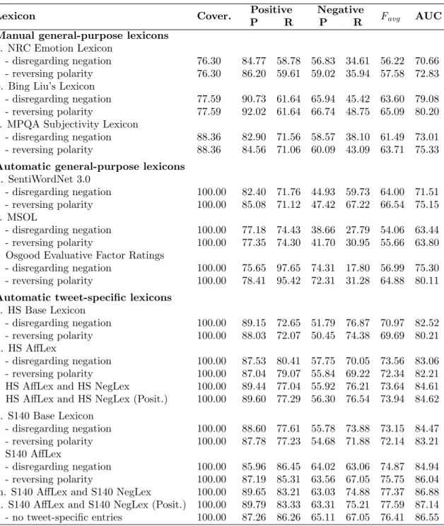
6.2.1 Lexicon Performance in Unsupervised Sentiment Analysis

In this set of experiments, we evaluate the performance of each individual lexicon on the message-level sentiment analysis task in unsupervised settings. No training and/or tuning is performed. Since most of the lexicons provide the association scores for the positive and negative classes only, in this subsection, we reduce the problem to a two-way classification task (positive or negative). The SemEval-2013 tweet test set and SMS test set are used for evaluation. The neutral instances are removed from both datasets.