HAL Id: insu-01352502
https://hal-insu.archives-ouvertes.fr/insu-01352502
Submitted on 6 May 2017
HAL is a multi-disciplinary open access
archive for the deposit and dissemination of
sci-entific research documents, whether they are
pub-lished or not. The documents may come from
teaching and research institutions in France or
abroad, or from public or private research centers.
L’archive ouverte pluridisciplinaire HAL, est
destinée au dépôt et à la diffusion de documents
scientifiques de niveau recherche, publiés ou non,
émanant des établissements d’enseignement et de
recherche français ou étrangers, des laboratoires
publics ou privés.
particles in the high Arctic marine boundary layer
Julia Burkart, Megan D. Willis, Heiko Bozem, Jennie L. Thomas, Kathy S.
Law, Peter Hoor, Amir A. Aliabadi, Franziska Köllner, Johannes Schneider,
Andreas Herber, et al.
To cite this version:
Julia Burkart, Megan D. Willis, Heiko Bozem, Jennie L. Thomas, Kathy S. Law, et al.. Summertime
observations of elevated levels of ultrafine particles in the high Arctic marine boundary layer.
Atmo-spheric Chemistry and Physics, European Geosciences Union, 2017, 17, pp.5515-5535.
�10.5194/acp-17-5515-2017�. �insu-01352502�
www.atmos-chem-phys.net/17/5515/2017/ doi:10.5194/acp-17-5515-2017
© Author(s) 2017. CC Attribution 3.0 License.
Summertime observations of elevated levels of ultrafine particles in
the high Arctic marine boundary layer
Julia Burkart1, Megan D. Willis1, Heiko Bozem2, Jennie L. Thomas3, Kathy Law3, Peter Hoor2, Amir A. Aliabadi4, Franziska Köllner5, Johannes Schneider5, Andreas Herber6, Jonathan P. D. Abbatt1, and W. Richard Leaitch7
1Department of Chemistry, University of Toronto, Toronto, Canada
2Institute of Atmospheric Physics, Johannes Gutenberg-University, Mainz, Germany 3LATMOS/IPSL, UPMC Univ. Paris 06 Sorbonne Universités, UVSQ, CNRS, Paris, France 4Environmental Engineering Program, University of Guelph, Guelph, Canada
5Particle Chemistry Department, Max Planck Institute for Chemistry, Mainz, Germany
6Alfred Wegener Institute, Helmholtz Center for Polar and Marine Research, Bremerhaven, Germany 7Environment and Climate Change Canada, Toronto, Ontario, Canada
Correspondence to:Julia Burkart ([email protected]) Received: 4 August 2016 – Discussion started: 8 August 2016
Revised: 27 February 2017 – Accepted: 28 February 2017 – Published: 2 May 2017
Abstract. Motivated by increasing levels of open ocean in the Arctic summer and the lack of prior altitude-resolved studies, extensive aerosol measurements were made during 11 flights of the NETCARE July 2014 airborne campaign from Resolute Bay, Nunavut. Flights included vertical pro-files (60 to 3000 m above ground level) over open ocean, fast ice, and boundary layer clouds and fogs. A general conclu-sion, from observations of particle numbers between 5 and 20 nm in diameter (N5−20), is that ultrafine particle formation
occurs readily in the Canadian high Arctic marine bound-ary layer, especially just above ocean and clouds, reaching values of a few thousand particles cm−3. By contrast, ultra-fine particle concentrations are much lower in the free tropo-sphere. Elevated levels of larger particles (for example, from 20 to 40 nm in size, N20−40)are sometimes associated with
high N5−20, especially over low clouds, suggestive of aerosol
growth. The number densities of particles greater than 40 nm in diameter (N>40)are relatively depleted at the lowest
al-titudes, indicative of depositional processes that will lower the condensation sink and promote new particle formation. The number of cloud condensation nuclei (CCN; measured at 0.6 % supersaturation) are positively correlated with the numbers of small particles (down to roughly 30 nm), indicat-ing that some fraction of these newly formed particles are capable of being involved in cloud activation. Given that the summertime marine Arctic is a biologically active region, it
is important to better establish the links between emissions from the ocean and the formation and growth of ultrafine par-ticles within this rapidly changing environment.
1 Introduction
Surface temperatures within the Arctic are rising almost twice as fast as in any other region of the world. As a mani-festation of this rapid change the summer sea ice extent has been retreating dramatically over the past decades with the possibility that the Arctic might be ice free by the end of this century (Boé et al., 2009) or even earlier (Wang and Overland, 2012). Arctic aerosol is well known to show a dis-tinct seasonal variation with maximum mass concentrations and a strong long-range anthropogenic influence in winter and early spring. The phenomenon, known as Arctic Haze, was identified many years ago (e.g. Barrie, 1986; Heintzen-berg, 1980; Rahn et al., 1977; Shaw, 1995), and has com-manded renewed attention in recent years (e.g. Law et al., 2014; Quinn et al., 2007). During summer the Arctic is more isolated from remote anthropogenic sources and represents a comparatively pristine environment. The reason is that the Arctic front (e.g. Barrie, 1986), which provides a meteo-rological barrier for lower-level air mass exchange, moves north of many source regions during the summer months.
Anthropogenic and biomass burning aerosols are transported to the Arctic during the summer, but increased aerosol scav-enging helps maintain the pristine conditions near the surface (e.g. Browse et al., 2012; Croft et al., 2016a; Garrett et al., 2011).
Zhang et al. (2010) discussed the impacts of declining sea ice on the marine planktonic ecosystem, which includes in-creasing emissions of dimethyl sulfide (DMS) that may con-tribute to particle formation in the atmosphere (e.g. Charlson et al., 1987; Pirjola et al., 2000). Enhanced secondary organic aerosol from emissions of biogenic volatile organic com-pounds is also a possibility (Fu et al., 2009). Primary emis-sions of aerosol particles from the ocean, such as sea salt and marine primary organic aerosol, may also increase (Browse et al., 2014). Open water tends to increase cloudiness, which means that aerosol influences on clouds are likely to be more important. Over the Arctic the effects of aerosols on clouds are especially uncertain. Models have predicted that increas-ing numbers of particles may lead to overall warmincreas-ing (Gar-rett, 2004) when the atmosphere exists in a particularly low particle number state now referred to being “cloud conden-sation nuclei (CCN) limited” (Mauritsen et al., 2011), to an overall cooling effect when increasing numbers of parti-cles are added to an atmosphere with more partiparti-cles already present (Lohmann and Feichter, 2005; Twomey, 1974). It is important to characterise particle size distributions in this pristine environment to provide a baseline against which fu-ture measurements can be compared in a warming world. Indeed, Carslaw et al. (2013) highlighted the need to un-derstand pre-industrial-like environments with only natural aerosols in order to reduce the uncertainty in estimations of the anthropogenic aerosol radiative forcing.
Primary sources, gas-to-particle formation processes, cloud processing, atmospheric ageing, mixing and deposition are all reflected in the size distribution. Therefore, measure-ments of aerosol size distributions are important for under-standing the processes particles undergo in addition to their potential effects on clouds. The presence of ultrafine parti-cles (UFPs) indicates recent production as their lifetime is of the order of hours. We focus this paper on ultrafine particles as these are an indication for in situ aerosol production pro-cesses in the Arctic. We also consider the growth of newly formed particles, as that determines how important they are for climate.
Aerosol size distributions including ultrafine particles (dp < 20 nm) have been measured before at different loca-tions throughout the Arctic. Long-term studies at ground sta-tions such as Alert, Nunavut (Leaitch et al., 2013), Ny Ale-sund and Zeppelin (Engvall et al., 2008a; Ström et al., 2003, 2009; Tunved et al., 2013), both on Svalbard and very re-cently in Tiksi, Russia (Asmi et al., 2016), and Station Nord, Greenland (Nguyen et al., 2016), indicate a strong seasonal dependence of the size distribution with the accumulation-mode aerosol dominating during the winter months and a shift to smaller particles during the summer months. New
particle formation events are frequently observed from June to August. Ström et al. (2003) showed that the size distribu-tion undergoes a rapid change from an accumuladistribu-tion mode dominated distribution during the winter months to an Aitken mode dominated distribution at the beginning of summer. To-tal number concentrations increase at the beginning of sum-mer and roughly follow the incoming solar radiation on a seasonal scale suggesting that photochemistry is an impor-tant factor for new particle formation in the Arctic. At Ny Alesund maximum number concentrations occur in late sum-mer and are explained by the Siberian tundra being a poten-tial source of aerosol precursor gases (Ström et al., 2003) and marine biogenic sulfur (Heintzenberg and Leck, 1994). Anal-ysis of air mass patterns for this region show that the shift in the size distributions is also accompanied by a change of source areas, with a dominance of Eurasian source areas in winter and North Atlantic air during summer (Tunved et al., 2013).
Particle measurements including aerosol size distributions were also conducted from ice breaker cruises such as from the Swedish ice breaker Oden (Bigg and Leck, 2001; Covert et al., 1996; Heintzenberg and Leck, 2012; Leck and Bigg, 2005; Tjernström et al., 2014) and the Canadian Coast Guard Ship ice breaker Amundsen (e.g. Chang et al., 2011). Chang et al. (2011) used model calculations to show that the appear-ance of ultrafine particles can be explained by nucleation and growth attributed to the presence of high atmospheric and oceanic DMS concentrations measured at the same time. The Odenexpeditions focus on the pack-ice-covered high Arctic, mainly north of 80◦N and also confirm the frequent presence of an UFP mode (e.g. Covert et al., 1996). The observations from the Oden cruises offer evidence that UFP in the inner Arctic might originate from primary sources (e.g. Heintzen-berg et al., 2015; Karl et al., 2013). This is motivated by three main observations. First, a lack of sulfuric acid compo-nents in collected 15–50 nm particles (Leck and Bigg, 1999). Second, Leck and Bigg (2010) highlighted that nucleation events in the high Arctic do not follow the classical banana shaped growth curve (Kulmala et al., 2001) but enhanced lev-els of ultrafine particles rather appear simultaneously in dis-tinct size ranges (Karl et al., 2012). Third, such events could not be modelled with the selected empirical nucleation mech-anism for the extremely low DMS concentrations in this re-gion (Karl et al., 2013). As a primary source, it is suggested that marine microgels might become airborne via the evapo-ration of fog and cloud droplets (Heintzenberg et al., 2006; Karl et al., 2013).
So far most studies that include size distribution mea-surements in the summertime Arctic were conducted from ground stations or ship cruises. To date there are only two studies that assess the altitude dependence of the size dis-tribution, i.e. one in the area of Svalbard (Engvall et al., 2008b) and one from the Oden performing vertical profiles with a helicopter (Kupiszewski et al., 2013). Although no size distribution measurements were performed,
Heintzen-berg et al. (1991) measured vertical profiles of the total parti-cle number concentration greater than 10 nm during June and July 1984 over the Fram Strait–Spitsbergen area, and found a “rather uniform distribution” with altitude. Their measure-ments, however, were confined to 500 m a.s.l. and above.
In this study we present data from aerosol size distribution measurements taken from an aircraft during a 3 week pe-riod in July 2014 in the high Arctic area of Resolute Bay, Nunavut, Canada. The flights focused on vertical profiles from as low as 60 m above the ground up to 3 km, as well as on low-level flights above different terrain such as fast ice, open ocean, polynyas and clouds. We focus especially on UFP (5–20 nm in diameter) and address the following questions: what are the concentrations of UFPs in the Arc-tic summertime, and what is their verArc-tical distribution? What are the environmental conditions that favour occurrence of UFPs and is there evidence for growth of UFP to CCN sizes? Aside from the studies conducted near Svalbard, we believe this is the first aircraft study in the high Arctic to systemat-ically address these specific questions. This work provides a comprehensive picture of UFPs observed during the cam-paign whereas a prior publication from Willis et al. (2016) detailed one UFP formation and growth event observed over Lancaster Sound.
2 Experimental
2.1 Sampling platform Polar 6
The research aircraft Polar 6 owned by the Alfred Wegener Institute, Helmholtz Center for Polar and Marine Research, Bremerhaven, Germany, served as the sampling platform. The Polar 6 is a converted DC-3 airplane (Basler BT-67) modified to work under extreme cold weather conditions. An advantage of the plane is that flights at very relatively low speeds and altitudes (< 60 m a.g.l.) are possible. The cabin of the aircraft is non-pressurised. We maintained a constant survey speed of approximately 120 knots (222 km h−1)for measurement flights at constant altitude, and ascent and de-scent rates of 150 m min−1for vertical profiles. Instruments and measurements specific to this paper are described below. Inlets
Aerosol was sampled through a stainless steel inlet mounted to the top of the plane and ahead of the engines to exclude contamination. The tip of the inlet consisted of a shrouded diffuser that provided nearly isokinetic flow. Inside the cabin the intake tubing was connected to a stainless steel tube (outer diameter of 2.5 cm, inner diameter of 2.3 cm) that car-ried the aerosol to the back of the aircraft where it was al-lowed to freely exhaust into the cabin so that the system was not over-pressured. The stainless steel tube functioned as a manifold, off which angled inserts were used to connect sam-ple lines to the various instruments described below. In-flight
air was pushed through the line with a flow rate of approxi-mately 55 L min−1determined by the sum of the flows drawn by the instruments (35 L min−1), plus the flow measured at the exhaust of the sampling manifold (20 L min−1). A flow of 55 L min−1was estimated to meet nearly isokinetic sam-pling criteria at survey speed and the transmission of particles through the main inlet was approximately unity for diameters between 20 nm to 1 µm (Leaitch et al., 2016). Although the transfer of the aerosol from outside to the instruments is rel-atively fast (5 s or less), volatilisation of some components of the particles may have occurred. However, the growth of newly formed particles by organic condensation occurs pri-marily by low volatility organic components (e.g. Pierce et al., 2012). Thus, the integrity of the smaller particles is likely to have been maintained. We do expect increasing line losses of particles with sizes decreasing from 10 nm. Therefore, our observations will underestimate N5−20.
Trace gases (CO and H2O) were sampled through a
sep-arate inlet made of a 0.4 cm (outer diameter) Teflon tube entering the aircraft at the main inlet and exiting through a rear-facing 0.95 cm exhaust line that provided a lower line pressure. The sample flow of approximately 12 L min−1was continuously monitored.
2.2 Instrumentation
2.2.1 Meteorological parameters and state parameters Aircraft state parameters and meteorological measurements were performed with an AIMMS-20 manufactured by Aven-tech Research Inc. at a very high sampling frequency (> 40 Hz). The AIMMS-20 consists of three modules: (1) the air data probe that measures the three-dimensional (3-D) aircraft-relative flow vector (true air speed, angle-of-attack and sideslip) and turbulence with a 3-D accelerometer; fur-thermore, temperature and humidity sensors are contained within this unit and provide an accuracy and resolution of 0.30 and 0.01◦C for temperature and 2.0 and 0.1 % for rel-ative humidity measurements; (2) an inertial measurement unit that consists of three gyros and three accelerometers providing the aircraft angular rate and acceleration; (3) A Global Positioning System for aircraft 3-D position and iner-tial velocity. Horizontal and vertical wind speeds were mea-sured with accuracies of 0.50 and 0.75 m s−1, respectively. The high-frequency raw data were processed to 1 Hz resolu-tion. Further details of the AIMMS including data processing can be found in Aliabadi et al. (2016a).
2.2.2 Aerosol physical and chemical properties
Particle number concentrations and particle size distributions were measured with a TSI 3787 water-based ultrafine con-densation particle counter (UCPC), a Droplet Measurement Technology (DMT) Ultra-High Sensitivity Aerosol Spec-trometer (UHSAS) and a Brechtel Manufacturing
Incorpo-rated (BMI) scanning mobility system (SMS) coupled with a TSI 3010 condensation particle counter (CPC). The UCPC detected particle concentrations of particles larger than 5 nm in diameter with a time resolution of 1 Hz. The flow rate was set to 0.6 L min−1. The particle concentrations measured by the UCPC are hereafter referred to as Ntot, noting as above
that diffusional losses of particles smaller than 10 nm deter-mine the lower limits of the Ntotobservations.
The BMI SMS was set to measure particle size distribu-tions from 20 to 100 nm with a sample flow of 1 L min−1and a sheath flow of 6 L min−1. The duration of one scan was 40 s with a 20 s delay time before each scan resulting in a time resolution of 1 min. The UHSAS performed size distri-bution measurements from 70 nm to 1 µm at a time resolution of 1 Hz with a sample flow rate of 55 cm3min−1. Details of the calibrations and instrument inter-comparisons performed prior to and during the campaign are described in detail in Leaitch et al. (2016).
CCN were measured with a DMT CCN counter (CCNC). The CCNC was operated behind a constant pressure inlet that was set to 650 hPa. The nominal supersaturation was held constant at 1 %. Calibrations prior to and during the cam-paign (for details see Leaitch et al., 2016) showed that a nom-inal supersaturation of 1 % at the reduced pressure translated into 0.6 % effective supersaturation.
Cloud droplet sizes from 2 to 45 µm were measured using a wing mounted particle measuring system FSSP 100. In this study these data are only used to identify periods when the aircraft was flying in clouds. To avoid possible artefacts pro-duced from shattering of cloud droplets at the aerosol inlet, data from in-cloud times are discarded for the purposes of this study.
A DMT single-particle soot photometer (SP2) was de-ployed to measure refractory black carbon (rBC) number and mass concentrations. We refer to rBC mass concentra-tions as an indication of pollution influence. Calibraconcentra-tions with Aquadag soot were performed prior to and during the campaign. The lower size limit of detection of rBC particles by the SP2 was approximately 80 nm.
Sub-micron aerosol composition was measured with an Aerodyne high-resolution time-of-flight aerosol mass spec-trometer (HR-ToF-AMS; e.g. DeCarlo et al., 2006). A de-tailed description of the instrument is found in Willis et al. (2016). The main purpose of the instrument was to mea-sure non-refractory particulate matter such as sulfate, nitrate, ammonium, methane sulfonic acid (MSA) and the sum of or-ganics. Detection limits were 0.009, 0.008, 0.004, 0.005 and 0.08 µg m−3, respectively, for a 30 s averaging time.
2.2.3 Trace gases
Carbon monoxide (CO) was measured with an Aerolaser ultra-fast carbon monoxide monitor model AL 5002 based on vacuum ultraviolet (VUV) fluorimetry, employing the ex-citation of CO at 150 nm. In situ calibrations were performed
during flight at regular intervals (15–30 min) using a National Institute of Standards and Technology (NIST) traceable CO standard with zero water vapour concentration. CO mixing ratios were used as a relative indicator of aerosol influenced by pollution sources.
Water vapour (H2O) measurements were based on infrared
absorption using a LI-7200 enclosed CO2/H2O Analyzer
from LI-COR Biosciences GmbH. The measurement uncer-tainty is ± 15 ppmv. H2O mixing ratios were used to
calcu-late relative humidity with pressure and temperature mea-sured by the AIMMS-20.
2.3 Data analysis and nomenclature of particle size data
All particle data were averaged to 1 min intervals to match the time resolution of the BMI SMS. Particle concentrations within different size intervals were calculated. The notation Na−b is used; “a” gives the lower limit and “b” the upper
limit of the calculated size interval. The BMI SMS was used to determine concentrations of particles from 20 to 90 nm in diameter, and concentrations of particles larger than 90 nm in diameter were determined by the UHSAS. If the size interval is expressed as N>athe upper limit is given by the detection
limit of the UHSAS (1 µm). Additionally, particle concentra-tions from 5 to 20 nm (short: N5−20)were obtained by
sub-tracting particle concentrations measured by the BMI SMS and by the UHSAS from the Ntotas determined by the CPC.
The N5−20are also referred to as ultrafine particles (UFP) in
this study and may be indicative of newly formed particles. Willis et al. (2016) showed that for this environment particles were able to grow to 50 nm low above the open water over approximately 1 h, which means that the growth from 1 to 10 nm can occur over approximately 1 min or less, justifying our use of instruments that are sensitive to 5 nm particles and larger. For the concentration range of N5−20 particles (less
than 2000 cm−3), it requires more than 30 h for the concen-tration of 10 nm particles to be reduced by coagulation to a concentration of 500 cm−3(Agranovski 2010).
In order to obtain vertical profiles the data were averaged within altitude intervals. An average profile for a single flight was obtained by binning all data from the respective flight into altitude intervals of 100 m starting at the lowest flight altitude. In addition to data obtained during vertical profile flights, data acquired while flying at a constant level were also included. Average profiles containing data from more than one flight were calculated by averaging the respective single flight profiles.
Average size distributions were obtained by simply aver-aging each bin for the desired time and altitude range. The size distributions measured by the BMI SMS were used for particle sizes from 20 to 90 nm, and the distributions at larger sizes are taken from the UHSAS. All particle concentrations are expressed for ambient pressure conditions, i.e. they have not been adjusted to standard temperature and pressure
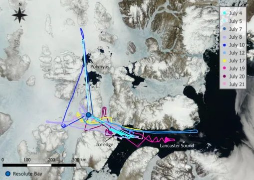
con-Figure 1. Compilation of all flight tracks plotted on a satellite image from 4 July 2014. The image is taken from https://earthdata.nasa.gov/ labs/worldview.
ditions. The N5−20 referred to as UFP are added to the size
distributions as additional bin assuming a bin width of 15 nm (from 5 to 20 nm) with a mid-diameter of 12 nm.
2.4 FLEXPART-WRF Simulations
We used FLEXPART-WRF (Brioude et al., 2013; web-site: http://flexpart.eu/wiki/FpLimitedareaWrf) simulations run backwards in time to analyse the origins of air masses sampled along the flight tracks. FLEXPART-WRF is a La-grangian particle dispersion model based on FLEXPART (Stohl et al., 2005). Meteorological information is obtained from the Weather Research and Forecasting (WRF) model (Skamarock et al., 2005). FLEXPART-WRF outputs retro-plume information such as the residence time of air (over a unit area) prior to sampling. Residence times were in-tegrated over the entire atmospheric column and 7 days backwards in time. FLEXPART-WRF was run in two ways. First, one FLEXPART-WRF was completed for each flight using particle releases every 2 min along the flight track (100 m × 100 m × 100 m centred on the aircraft location) to produce potential emissions sensitivities that represent the average air mass origin for each flight. Second, separate runs were completed for points (every 10 min) along the flight track (100 m × 100 m × 100 m, 60 s release duration) in or-der to study different air masses measured during the same flight. A more detailed description of the model as used for NETCARE 2014 is provided by Wentworth et al. (2016).
2.5 Study area and flight tracks
From 4 to 21 July 2014 11 flights were conducted out of Res-olute Bay (74.7◦N, 95.0◦W). In Fig. 1 a compilation of all flight tracks on a satellite image is shown. The satellite pic-ture was taken on 4 July 2014 and reflects the situation of the region during period I (4 to 12 July). Resolute Bay proved to be an ideal location for this study as we had access to both open ocean and ice-covered regions. Additionally, two polynyas were located north of Resolute Bay within the reach of our aircraft. Flights ranged between 4 and 6 h. The flights covered two main areas: Lancaster Sound east of Resolute Bay and the area north of Resolute Bay, where two polynyas were located. The flights south of Resolute Bay in Lancaster Sound concentrated around the ice edge.
The ice/water coverage visible on the satellite picture is representative for the area during the first period. As can be seen, the ice edge was situated about 150 km east of Resolute Bay. It is clearly visible in the satellite image as a sharp line. The transition from a completely ice-covered region to open ocean was very abrupt during the first period. Only after a period of bad weather with high winds did the ice edge be-come less clear, and the region starting about 80 km east of Resolute Bay to about 200 km east was covered by fractured ice.
Roughly 50 % of the flight time was within the inversion layer, and 50 % was in the free troposphere conducting alti-tude profile flights. A considerable amount of time was spent at 2800 m as this was the preferred altitude when travelling to a certain area. When clouds were present, the aircraft
sam-Figure 2. Median temperature, relative humidity (RH), wind speed, CO mixing ratio and Ntotprofiles for the Arctic air mass period (dark
red), the transition day (dark green), and the southern air mass period (dark blue). Median profiles for each flight are plotted in the background in the corresponding light colours.
pled them by slant profiling through the cloud in the case that clouds were above the boundary layer, or in the case clouds were within 200 m of the surface, by descending into the cloud as low as possible. Aerosol observations while inside cloud are excluded from the analysis here due to potential artefacts from droplets shattering on the outside inlet.
3 Meteorological and atmospheric conditions
Meteorological conditions changed over the course of the campaign. Similar conditions were encountered during the first part of the campaign (4–12 July, 6 flights), referred to as the “Arctic air mass period” because air masses from within the Arctic dominated and the atmosphere showed structures typical for the Arctic, such as a low boundary layer height with thermally stable conditions, indicated by a near-surface temperature inversion and frequent formation of low-level clouds. At this time Resolute Bay was under the influence of high-pressure systems. Clear sky with few or scattered clouds and low wind speeds dominated. Conditions changed starting from 13 July when the region was influenced by troughs of a low-pressure system located to the west above Beaufort Sea, which eventually passed through Resolute Bay on 15 July bringing along humidity, precipitation and fog. Intense fog and low visibility impeded flying from 13 to 16 July. A short good weather window in which the fog dissipated permitted flying again on 17 July (referred to as “transition day”; one flight) just before Resolute Bay came under influence of a pronounced low-pressure system located to the south with its centre around King William Island (69.0◦N, 97.6◦W). The last campaign days (referred to as “southern air mass period”, three flights) were characterised by the influence of this pro-nounced low-pressure system bringing air masses from the
south and providing higher wind speeds, an overcast sky and occasional precipitation.
Vertical profiles of median temperature, relative humid-ity (RH), wind speed, CO and Ntot (Fig. 2) illustrate
me-dian atmospheric conditions during the measurement flights. Prominent features representing the trend of each period and reflecting the general meteorological situation will be de-scribed here, with details discussed in the respective sections. The Arctic air mass period was characterised by frequent thermally stable conditions within the near-surface layer, rep-resenting typical conditions during the Arctic summertime (Aliabadi et al., 2016a; Tjernström et al., 2012). The median temperature profiles show that on average the boundary layer reached up to ∼ 300 m with a temperature increase of about 5◦C. In this paper we will refer to this part of the atmosphere as the boundary layer (BL) and to the air masses above as the free troposphere (FT). A BL height of 300 m corresponds well to the boundary layer height of 275 m ± 164 m esti-mated by (Aliabadi et al., 2016a) using the method of bulk Richardson number (Aliabadi et al., 2016b) with a critical bulk Richardson number of 0.5, using data from radioson-des launched at Resolute Bay and the Amundsen icebreaker, which also performed research operations in Lancaster sound during the campaign period.
Within the BL, particle concentrations spanned over a wide range of concentrations (max Ntot: ∼ 10 000; median
values: ∼ 150 to ∼ 1700 cm−3). The highest Ntot occurred
during the Arctic air mass period, while Ntot was
con-stantly low within the lower atmosphere on the transition day. Median temperatures near the surface ranged from −1 to 5◦C during the Arctic air mass period, largely depend-ing on the terrain below (e.g. ice or open water) and were clearly higher when the southern air masses arrived (e.g. at the “surface”: 4 and 7◦C, respectively) and, if present, the BL was less pronounced. The higher temperatures
co-incide with the influence of low-pressure systems bringing warmer air masses from the west and south, and additional higher wind speeds providing a better mixing of the atmo-spheric layers (5.6 m s−1 vs. 12 m−1 near the surface). CO mixing ratios were extremely low during the Arctic air mass period (median: 78.3 ppbv)and on the transition day
(me-dian: 83.4 ppbv)indicating pristine air masses that had not
re-cently been affected by pollution or biomass burning sources. During the southern air mass influence, CO mixing ratios clearly increased (median: 95.0 ppbv)confirming a change
in air mass and suggesting possible influences by pollution sources and wild fires in the North West Territories (Fig. S2 in the Supplement). Relative humidity profiles show that the near-surface layer of the atmosphere was very moist with RH > 80 % during all periods.
4 Results and discussion 4.1 Ultrafine particle events
4.1.1 Frequency of ultrafine particle events
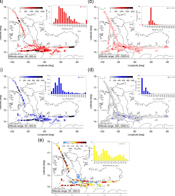
Throughout the campaign we observed large variability in particle concentrations (Fig. 3). We observed not only very clean air masses with Ntot of a few tens of cm−3 (with
the lowest 1 s value of 1 cm−3), but also concentrations as high as a few thousands per cm−3 (with the highest value of 10 000 cm−3). The highest and lowest concentra-tions were measured within the BL (Fig. 3b). Above the BL (Fig. 3b) particle concentrations were relatively constant where 60 % of the time concentrations were between 200 and 300 cm−3(for a discussion of the average size distribution see Sect. 4.1.2–4.1.4). Especially during the Arctic air mass period (Fig. 2) the atmosphere was characterised by a strong contrast between the BL and the FT.
UFP were very frequently present within the BL in high concentrations (Fig. 3c). Here we refer to “bursts” of par-ticles as a sudden and relatively large increase in N5−20:
concentrations suddenly rising from tens of cm−3 to sev-eral hundreds and thousands cm−3. This may reflect inho-mogeneities in the UFP formation process or reflect the air-craft flying in and out of areas of high UFP concentrations. Bursts of N5−20> 2000 cm−3were observed over polynyas,
which were consistent with previous observations (Leaitch et al., 1984, 1994), in Lancaster Sound and south of Reso-lute Bay. The N5−20was higher than 200 cm−3during 65 %
of the time. Indeed, high Ntotwas mainly driven by UFP (as
can be seen by comparison of black dots indicating high Ntot
in Fig. 3c and high UFP in Fig. 3d). Whenever Ntotis greater
than 2000 cm−3, UFP was larger than 1000 cm−3. This is also illustrated by the ratio of UFP/Ntot (Fig. 3e). A ratio
of zero means that no UFP were present, while a ratio of 1 means that only UFP were present. Within the boundary
layer 32 % of the time the size distribution was dominated by UFP (ratio > 0.5).
The frequent presence of UFP agrees well with other stud-ies made during the Arctic summertime at several locations, such as at the ground stations in Ny Alesund and Zeppelin (Ström et al., 2009; Tunved et al., 2013), at Alert (Leaitch et al., 2013), and from ship-based observations (Chang et al., 2011; Covert et al., 1996; Heintzenberg et al., 2006). How-ever, such a frequent presence of an UFP mode (65 % of the time > 200 cm−3)in the BL is unique to this study. Possible reasons for the higher occurrence of UFP might be the com-bination of the proximity of open ocean (providing a source of UFP or precursor gases), favourable meteorological con-ditions (sunny weather, inversion layer with cloud forma-tion) and very clean air masses with low condensation sinks. Also, since observations of UFP were one focus of this study, the fractional occurrence of the UFP mode may be biased slightly high due to longer sampling times associated with UFP occurrence. Calm weather conditions may have been another factor. The highest concentrations of UFP were mea-sured at lower wind speeds (< 5 m s−1; Fig. S1), while lower UFP concentrations (1000 cm−3)were found at higher wind speeds (> 12 m s−1)suggesting a dilution effect of the wind. Such a dilution effect implies proximity to the source.
In the following sections, the vertical distribution of UFP and the size distributions are discussed in relation to mete-orological conditions during the three distinct periods that characterised this campaign.
4.1.2 Arctic air mass period: 4 July to 12 July
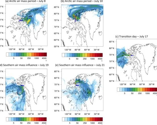
During this first period the study area was under the influence of a high-pressure system. As illustrated by FLEXPART-WRF results (Fig. 4a and b), air masses were either coming from the north extending to the east in the Arctic Ocean or from the east passing over the open ocean in Lancaster Sound and Baffin Bay. Both examples indicate that air masses resided within the Arctic region at least 5 days prior to sam-pling. This is true for all flights during this period. The very low CO mixing ratios (78 ppbv; see Fig. 2) and average BC
mass concentrations of 3 ng m−3(not shown) confirm that air masses were very clean and without recent influence from pollution sources. As discussed in Sect. 3, temperature pro-files indicate thermally stable conditions in the lowest lay-ers with near-surface temperature invlay-ersions. During almost all vertical profiles, we observed temperature inversions of about 4–6◦C near the surface. Such an atmospheric
struc-ture, i.e. a shallow boundary layer, is typical for the Arctic summertime (e.g. Aliabadi et al., 2016a; Tjernström et al., 2012).
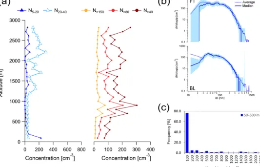
The Arctic air mass period was characterised by a very sharp contrast between the BL and the FT in terms of par-ticle number concentrations and sizes (Fig. 5). The BL was characterised by a prominent layer of UFP from the surface to about 300 m with the highest concentrations closest to the
Figure 3. Flight tracks colour coded by particle concentrations. (a) Flight tracks within the boundary layer (50–300 m) colour coded by Ntot. (b) Flight tracks within the free troposphere (300–3000 m) colour coded by Ntot. (c) Flight tracks within the boundary layer (50–
300 m) colour coded by UFP. (d) Flight tracks within the free troposphere (300–3000 m) colour coded by N5−20. (e) Flight tracks within the
Figure 4. FLEXPART-WRF potential emissions sensitivities for each flight (using particle releases every 2 min along the flight track) that illustrate transport regimes during different periods of the campaign. The colour code indicates the residence time of air in seconds and the numbers represent the position of the plume centroid location in days prior to release (days 1–7).
surface (Fig. 5a). The height of the UFP layer coincides with the average height of the temperature inversion for this period (see temperature profile Fig. 2) and indicates that air masses were stably layered limiting exchange with the FT. This is supported by the observed lower turbulent mixing (i.e. tur-bulent kinetic energy) from boundary layer to the free tropo-sphere during the campaign (Aliabadi et al., 2016a).
During this period we measured the highest concentrations of UFPs with the 1 min average up to 5300 cm−3. On a typi-cal flight several bursts (see Sect. 4.1.1) of high UFP concen-trations were encountered in the BL. Particle bursts lasted from a few seconds to several minutes, corresponding to a spatial extent of several hundreds of metres to dozens of kilo-metres. The large spatial variability is also illustrated by the frequency distribution of UFP in the BL shown in Fig. 5c; 40 % of the time concentrations of UFP were larger than 200 cm−3, 11 % of the time larger than 1000 cm−3and 3 % of the time even larger than 2000 cm−3. Particle concentra-tions in the FT are relatively uniform, and concentraconcentra-tions of UFP were less than 50 cm−3 up to 1200 m and ∼ 10 cm−3 above.
The average N20−40is similar to the UFP, showing a
max-imum in its concentration at the same altitude. The concen-trations of larger particles (N>40, N>80, N>150)are much
lower in the clean BL (surface areas of ∼ 5 µm2m−3 and
lower). However, the N>40and N>80increase from the
low-est altitude to the next averaged altitude, consistent with the increase in the UFP and N20−40. These results suggest that
some of the UFP experienced growth to sizes of 20–80 nm within a few hours, as demonstrated by Willis et al. (2016). Within the FT particle concentrations were surprisingly uni-form and concentrations of UFP were less than 50 cm−3up to 1200 m and ∼ 10 cm−3above 1200 m.
In Fig. 5b, the median size distribution shows that in-creases in UPF in the BL were frequent. The average size distribution shows that at times higher concentrations of par-ticles extended up to about 80 nm, consistent with the sug-gestion above that some UFP particles experienced growth to larger sizes. A relevant case will be discussed in Sect. 4.3. Occasionally a mode of particles larger than 400 nm was present in the BL over open water (see Sect. 4.2), which was likely the product of primary oceanic emissions.
4.1.3 Transition day on 17 July
17 July marks the transition from dominance by Arctic air masses to a more distant influence from southern air masses. The transition day consists of only one flight in the area of Lancaster Sound, during which low concentrations of parti-cles larger than 20 nm were observed below 600 m; e.g. N>40
Figure 5. Average particle concentration data during the Arctic air mass period. (a) Average vertical profiles of N5−20, N20−40, N>40, N>80
and N>150. (b) Average (solid line) and median (dashed line) size distribution within the BL and the FT. The light blue area represents the
25–75th % percentile range. (c) Frequency distribution of the occurrence of UFP illustrates the large variability of the UFP concentrations within the BL.
ranged from 60 to 100 cm−3; see Fig. 6. The deeper layer of lower concentrations may have been a result of cloud pro-cessing and scavenging. During the days prior to this flying was impossible because of intense fog and cloud at Resolute Bay. A different transport regime may also have contributed to this situation. On this day the low-pressure system situated to the west was bringing air masses from the west along the Canadian and Alaskan coastline (Fig. 4c). The temperature profile shows an inversion between 650 and 1000 m possibly indicating a change in air mass. CO mixing ratios (83 ppbv)
and BC mass concentrations (3 ng cm−3)were also quite low indicating mostly Arctic background conditions.
On this day, occasional bursts of UFP up to 1400– 1900 cm−3 were observed within the boundary layer (Fig. 6b). UFP of 200 cm−3 or more were observed about 20 % of the time (Fig. 6c), and the average concentration was 240 cm−3 at the lowest level of the profile (Fig. 6a). Concentrations of larger particles (N>40, N>80, N>150)
in-creased sharply at about 700 m, coinciding with the temper-ature inversion. The very low concentrations of larger par-ticles (N>150: < 10 cm−3) below the temperature inversion
are very similar to the conditions encountered within the BL during the previous period. As above, the differences in the transition day below 700 m may have been due to a com-bination of fog/cloud scavenging and a change of air mass. Median and average size distributions indicate a minimum at around 65 nm that might be the result of cloud processing (Hoppel et al., 1994), consistent with the Arctic observations
of Heintzenberg et al. (2006) and the activation diameters ob-served during this study (Leaitch et al., 2016).
4.1.4 Southern air mass period: 19 July–21 July During this period the region was under the influence of a low-pressure system centred south of Resolute Bay. FLEXPART-WRF air mass trajectories (Fig. 4d and e) in-dicate a prevalence of air masses from the south potentially affected by wild fires (see Fig. S2). At the beginning of this period on 19 July (Fig. 4d), air mass trajectories suggest the strongest influence from the south while towards the end of the period on 21 July (Fig. 4e) FLEXPART-WRF indicates that southern air masses mixed with air masses coming off Greenland. Near-surface temperatures were higher than dur-ing the previous periods (Fig. 2), and temperature inversions were less pronounced (2–4◦C) and not observed at all loca-tions suggesting a less stable lower atmosphere. On 19 July we encountered the highest wind speeds in the BL (16 m s−1 within the near-surface layer and 20 m s−1 slightly above). Furthermore, RH was relatively high near the surface (91 %) and did not drop below 80 % throughout the vertical atmo-sphere. CO mixing ratios were higher than during the prior periods suggesting that the air was at times influenced by pollution or biomass burning.
UFP were observed less frequently than during the Arctic air mass period and in lower concentrations (Fig. 7). Bursts of UFP above 1000 cm−3 occurred only at three locations, all during the flight on 21 July. Average UFP concentrations
Figure 6. Average particle concentration data on the transition day. (a) Average vertical profiles of N5−20, N20−40, N>40, N>80 and N>150. (b) Average (solid line) and median (dashed line) size distribution within the BL and the FT. The light blue area represents the
25–75th % percentile range. (c) Frequency distribution of the occurrence of UFP illustrates the large variability of the UFP concentrations within the BL.
Figure 7. Average particle concentration data during the southern air mass period. (a) Average vertical profiles of N5−20, N20−40, N>40, N>80and N>150. (b) Average (solid line) and median (dashed line) size distribution within the BL and the FT. The light blue area represents
the 25–75th % percentile range. (c) Frequency distribution of the occurrence of UFP illustrates the large variability of the UFP concentrations within the BL.
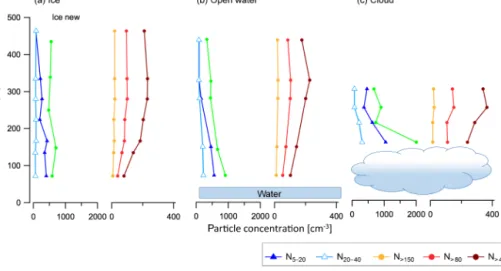
Figure 8. Average profiles of particle concentrations above ice, open water and cloud. The number of data points for each specific profile is 130 above water, 216 above cloud and 123 above water.
were only approximately 190 cm−3. UFP concentrations of 200 cm−3 or higher were detected 31 % of the time below 300 m (Fig. 7c).
The southern air mass period clearly shows different aerosol characteristics within the near-surface layer than compared to the Arctic air mass period and the transition day. Average concentrations of particles larger than 40 nm were the highest within the boundary layer and decreased with altitude (Fig. 7a). This is in sharp contrast to the cleaner boundary layers observed before. Whereas concentrations of particles larger than 40 nm were ∼ 100 cm−3and lower dur-ing both prior periods, they were as high as 300 cm−3for this period. Even large accumulation-mode particles (N>150)
av-eraged ∼ 50 cm−3(compared to 10 cm−3 for both previous periods). Moreover, both the median and average size dis-tributions show a pronounced mode of particles larger than 500 nm within the BL (Fig. 7b). Primary emissions from the sea spray promoted by the higher surface wind speeds (see Fig. 2) are likely a factor contributing to the larger particles. During the southern air mass period, three important fac-tors had changed compared to both prior periods. (1) Air mass back trajectories had clearly shifted to the south and po-tentially transported emissions from wild fires located in the Northwest Territories (Fig. S2) into the region, which might mix into the boundary layer. (2) The Amundsen ice breaker was present in Lancaster Sound and acted as a local pollu-tion source. (3) Wind speeds were higher and the ocean was visibly turbulent with breaking waves that might enhance pri-mary oceanic aerosol emissions. The increased condensation sinks from these potential sources in combination with other factors (e.g. reduced sun light) and relatively low residence times of air masses within the boundary layer (compared to the Arctic air mass period) may explain the relatively low and infrequent concentrations of UFPs.
Within the FT the size distributions shows a bimodal char-acter with a minima at 60–80 nm, which may indicate the air masses experienced cloud processing. This is likely, given the presence of the low-pressure system bringing moister and warmer air masses. The bimodal size distribution is different from the average size distribution during the Arctic air mass period when drier air masses from within the Arctic domi-nated.
4.2 UFP occurrence above ice vs. water
We investigated the potential influence of different under-lying water surfaces on the occurrence of UFP by examin-ing in detail the time periods when we were flyexamin-ing at alti-tudes at or below 500 m during the Arctic air mass period. We distinguish between three water surfaces: ice-covered ar-eas (including ice edge and ice covered with melt ponds), open ocean (including polynyas) and low-level clouds (in-cluding both cloud above water and cloud above ice). Here we point out that the case “cloud” does not include in-cloud flight times but only flight periods when above cloud top without actually entering the cloud (confirmed by a zero sig-nal in a liquid cloud probe, FSSP100). An altitude of 500 m was chosen to include time periods when we were flying above low-level clouds and to capture mostly flights within the boundary layer where a local influence of the terrain be-low was likely. During the Arctic air mass period, there was a clear separation between ice and open water over Lancaster Sound with east of the ice edge completely ice free, where west of the ice edge the ocean was seamlessly covered by fast ice (see satellite picture in Fig. 1).
Each average profile above the different water surfaces ex-hibits unique features (Fig. 8). Above ice the highest con-centrations of UFP (average: 400 cm−3)were found nearer the surface (70 m) and the Ntotare slightly higher (580). In
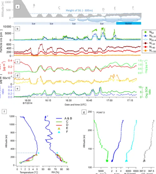
Figure 9. Case study from 8 July flight. Time series of flight altitude and illustration of the surface including cloud coverage (a), aerosol size (b) and chemical composition (c–e). (f) Vertical profiles of temperature and RH at locations A–F. (g) Ntot, temperature, H2O mixing
ratio and CO2profiles at location D.
the BL over open water, the Ntotand UFP number
concen-trations are 900 and 560 cm−3, respectively, and in the air just above cloud, the average Ntotand UFP number
concen-trations are 2000 and 1040 cm−3, respectively. In the open water and cloud cases, the highest concentrations of ultrafine particles are at the point of measurement closest to the water surface. In the cloud case and open water case, the N20−40
particles show an increase at the same time as the Ntotand
UFP suggesting that the UFP form and grow to larger sizes. This is not observed in the over-ice case, which suggests that some of the new particles could have formed elsewhere (e.g. over open water) and been transported over the ice, or that the growth rates over ice are slow. In all three cases, the largest particles show relatively smaller abundances at the lowest al-titudes samples. An increased abundance of UFP at lower surface areas supports the hypothesis that UFP form via nu-cleation of precursor gases.
4.3 Case study: 8 July
The flight on 8 July provides a case study illustrating that the occurrence of UFP is confined to the BL suggesting a surface source of UFP and that the appearance of UFP is promoted by cloud. We consider the altitude dependence of the UFP within the BL in relation to air mass history and cloud.
On this flight we first flew out into Lancaster Sound west of Resolute Bay, turned around and descended into the BL above the ice. Here, we focus on the time period from 15:50 UTC (descent into the BL) to 17:20 UTC where we travelled from west to east and remained within the BL but stayed out of cloud as shown in Fig. 9; see also Fig. S2. The later part of the flight focused on in situ cloud properties and is discussed elsewhere (Leaitch et al., 2016). The weather was sunny with low-level clouds starting around 150 km over ice and west of the ice edge in Lancaster Sound. The clouds
had formed over the water and were blown over the ice where they were dissipating (Leaitch et al., 2016). In the entire area the atmosphere was characterised by a surface temperature inversion extending vertically up to about 300 m with ∼ 1◦C near the surface and ∼ 5◦C at 300 m and was accompanied by decreasing relative humidity (Fig. 9f). Local low-level winds were predominantly from the south to east and wind speeds were below 5 m s−1.
UFP were present throughout the BL with the highest con-centrations at the lowest altitudes and decreasing concentra-tions towards the top of the BL (Fig. 9b). In contrast, larger particles (e.g. N>40)exhibit the opposite pattern, with lower
concentrations at lower altitudes and higher concentrations at higher altitudes. Six locations from west to east (points A–F in Fig. 9a) are used to illustrate the changing aerosol charac-teristics. Location A is situated well above the BL and at this point no UFP were present (detailed size distributions are shown in Fig. S4). At location B, the point at which we first entered the BL, an UFP mode (∼ 370 cm−3)was present at 60 m, while UFP concentrations were lower at slightly higher altitudes (∼ 80 cm−3at 230 m) such as at location C. At the lower altitudes the UFP concentrations gradually increased as we approached the ice edge. The most striking observation is the steep increase in particle concentrations at about 60 km west of the ice edge (location D), where UFP increased to above 4000 cm−3 at 150 m or just above cloud top. At the same time N20−40concentrations showed a similar increase.
The increased UFP concentrations were vertically limited to near cloud top and decreased rapidly with increasing altitude. The same pattern is also observed for temperature, H2O and
CO2(Fig. 9g) suggesting the existence of a distinct air mass
at the surface that gets diluted into the air mass above. Fur-ther east the flight was restricted to a slightly higher altitude above cloud top. At point F, where we were close to the BL top, no peaks in particle concentrations were observed. At point E, just before the ice edge, between the top of cloud and the top of the BL, UFP concentrations reached about 3400 cm−3.
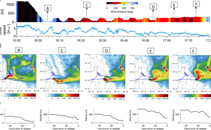
Air mass histories at these locations determined from FLEXPART-WRF (Fig. 10) indicate the following:
1. To the west of Resolute Bay (point B), Lancaster Sound air masses had been mixed with air masses from the north. This is also confirmed by the local wind direc-tions indicating winds coming from the northwest sec-tor (Fig. 10a), and it is consistent with the associated change in cloud.
2. Near the top of the BL, air masses had descended re-cently (< 3 h) into the BL (Fig. 10c point C and point F). 3. In contrast, deeper within the BL at points B and D, air masses had descended into the BL earlier (∼ 20 h) be-fore arriving at the point of observation. In the case of point D, where we observed the largest mode of UFP extending above 40 nm, air masses had been travelling
from the east exclusively over the open waters in Lan-caster Sound during the last day before arriving at the point of observation.
Aerosol composition shows a clear difference between the aerosol in the FT and the BL. The aerosol sulfate rapidly de-creases as we enter the BL around 16:00 UTC, while aerosol organic mass concentrations show an initial relative increase followed by an absolute increase towards the east (Fig. 9c). Within the BL, aerosol organics and sulfate mass loadings show a pattern similar to N>40 and N>80. Both decrease
each time we descended deeper into the BL. However, at the same time the organics-to-sulfate ratio indicates that the rel-ative contribution of organics to aerosol mass increases at lower altitudes and especially above cloud (Fig. 9e). Well within the inversion layer and in the vicinity of cloud top the aerosol was dominated by organics. At the same time, also the ratio of MSA to sulfate was higher (Fig. 9e), sug-gesting a marine biogenic influence of the aerosol sulfur. The marine biogenic influence at the lower altitudes agrees well with the FLEXPART-WRF simulations showing that air masses at this altitude had spent almost an entire day ex-posed to the open waters in Lancaster Sound. Consistent with the higher organic content measured with the AMS, the sin-gle particle aerosol mass spectrometer ALABAMA (Brands et al., 2011; Willis et al., 2016) detected a higher fraction of trimethylamine (TMA)-containing particles for particles larger than 150 nm in diameter (F. Köllner, personal commu-nication, July 2016). Gaseous TMA emissions from marine biogenic origin (Ge et al., 2011; Gibb et al., 1999) may have additionally favoured the subsequent growth of the freshly nucleated particles by condensation. Another possibility may be uptake of TMA in the cloud phase (Rehbein et al., 2011) if the particles have grown to sufficiently large sizes to be ac-tivated as CCN. Interestingly, compared to other days these TMA-containing particles are smaller and to a lesser degree internally mixed with potassium and levoglucosan, which supports the hypothesis of ultrafine particles originating from nucleation in a biogenic marine environment and subsequent growth.
To explain these observations, we hypothesise that the smaller particle mode is formed by nucleation and growth oc-curring within the BL and especially in cloud vicinity. UFP concentrations near cloud top have been reported before (e.g. Radke and Hobbs, 1991, Wiedensohler et al., 1997, Clarke et al., 1999; Garrett et al., 2002; Hegg et al., 1990; Mauldin et al., 1997) and it is suggested that nucleation in near-cloud regions is favoured by the low surface areas, possibly due to cloud scavenged aerosol, moist air and a high actinic flux. Indeed, near cloud top, where we observed an increase of UFP extending up to almost 50 nm, the conditions for nucle-ation and growth are ideal. We speculate that the availabil-ity of precursor gases is provided by the long residence time (∼ 20 h) of the air masses over open water (Fig. 10, point D). In other words, precipitating clouds scavenge aerosol
parti-Figure 10. (a) Time series of aircraft altitude colour coded with the wind direction and time series of wind speed. (b) FLEXPART-WRF 7-day-backwards potential emissions sensitivities for points along the flight track (60 s release at indicated time and location) showing the air mass history at five representative locations within the BL. The plume centroid location for particles with an age of 1 day is indicated. (c) The bottom plots show the altitude of plume centroid 48 h backwards in time.
cles, reducing the surface area for condensation, but some fraction of nucleation precursor gases with lower Henry’s law constants, can pass through (e.g. SO2)leaving the
poten-tial for H2SO4in the higher OH in the cloud outflow (a
dis-cussion of the processes can be found in Seinfeld and Pandis, 2016). The very high organic loadings and MSA-to-sulfate ratio likely indicate that the formation and growth of these particles is driven by a combination of DMS and organic precursors (volatile organic compounds) that are emitted by the open ocean in Lancaster Sound (e.g. Chang et al., 2011; Sjostedt et al., 2012; Mungall et al., 2016).
The event at point E occurs where the aircraft was be-tween cloud top and the top of the BL, where no increases in UFP were observed before or after. It may be that the aircraft descended slightly but sufficiently into the cloud-influenced area, which looks to be 25–40 m above cloud top (Fig. 9g), but also at that point we were in vicinity of Prince Leopold Island, which is a bird sanctuary and many bird colonies nest at the 260 m high cliff. FLEXPART-WRF and the in situ wind measurement show that air masses to a large extent were di-rectly coming off the island (Fig. 10, point E) suggesting a connection between the appearance of UFP and possible
emissions from the fauna of the island. The increase of parti-cle phase ammonium (Fig. 9d) at the same time supports this connection and nucleation of particles from biogenic precur-sors emitted by bird colonies are documented (Weber et al., 1998; Wentworth et al., 2016, Croft et al., 2016b).
Alternatively, it should be considered that evaporating fog and cloud droplets may also act as a primary source of UFP (e.g. Heintzenberg et al., 2006; Karl et al., 2013; Leck and Bigg, 1999). Karl et al. (2013) suggested a combined path-way that involves the emission of UFP by fog and cloud droplets, together with secondary processes enabling growth of these particles. For our observations we have no reason to assume that nucleation does not occur since conditions are ideal but we cannot rule out that nanoparticles are emitted by the possibly evaporating cloud droplets onto which gases then condense.
In conclusion the aerosol mass within the near-surface layer is dominated by organics relative to sulfate, while at just a slightly higher altitude sulfate is clearly increased and increases further above the inversion layer. A high organic content coincides with increases in UFP particles, especially at times when also growth into the size range up to 50 nm is
Figure 11. (a) Vertical profiles of average CCN concentrations (dark blue). All data points are plotted in light grey. (b) Correlation plots between CCN concentrations and particles larger than 80 nm.
indicated. Similarly the MSA-to-sulfate ratio shows a peak at the lowest altitudes with maximum values in the vicinity of clouds that coincide with a long residence time (∼ 20 h) of the air masses within the BL and above open water. The data thereby suggest a marine biogenic influence of the aerosol within the lower layers of the atmosphere. We note that simi-larly high levels of aerosol organics and MSA were observed during the flight on 12 July associated with a NPF event and growth but in cloud-free conditions (Willis et al., 2016). 4.4 CCN activity
CCN concentrations were measured at a supersaturation of 0.6 %. The vertical profiles of CCN concentrations (Fig. 11a) show patterns similar to those of larger particles. In the very clean boundary layer of the Arctic air mass period and the transition day CCN concentrations are equally low (∼ 70 and ∼50 cm−3, respectively). In contrast, southern air mass pe-riod average BL CCN concentrations are amongst the highest observed during this campaign (> 300 cm−3). Within the free troposphere, CCN concentrations are surprisingly constant during the Arctic air mass period (120 ± 27 cm−3)and more variable on the transition day (92 ± 46 cm−3)and the south-ern air mass period (103 ± 67 cm−3). The constant CCN con-centrations during the Arctic air mass period correspond to the very uniform atmosphere dominated by aged aerosols we
observed during this period and to the more layered atmo-sphere influenced by southern air masses possibly contam-inated by biomass burning plumes during the later period. Correlations with N>80(Fig. 11b) confirm that larger
parti-cles are a good approximation for these CCN concentrations. On average CCN concentrations agree to within ±20 % of N>80. However, it should be noted that slight differences
between the three periods are indicated in the correlation curves; during the Arctic air mass period, the average activa-tion diameters are smaller than 80 nm, and during the south-ern air mass period they are larger than 80 nm. Assuming uniform chemical composition throughout the particle size range, an activation diameter of 80 nm at 0.6 % supersatura-tion indicates an aerosol much less hygroscopic than, for ex-ample, ammonium sulfate; pure ammonium sulfate particles would activate at 40 m at 0.6 % supersaturation. For the one specific event during which growth occurred (Willis et al., 2016), it was demonstrated that high CCN concentrations co-incide with elevated organic mass loading. The reduced hy-groscopicity of organic material relative to soluble inorganic salts (Petters and Kreidenweis, 2007) can explain the larger effective activation diameter.
A central question is whether and to what degree the CCN are influenced by the UFP. Two factors help with addressing this question; (1) particles as small as 20 nm and in general much smaller than the average 80 nm size associated with
Figure 12. Correlations between CCN and particle concentrations for the full study period.
the CCN at 0.6 % will nucleate cloud droplets in the clean environment of the summer Arctic (Leaitch et al., 2016), and (2) there is evidence here that increases in particles larger than 20 nm are associated with increases in the UFP, partic-ularly for UFP influenced by clouds (e.g. Fig. 8). Figure 12 shows regressions of CCN with UFP, N>20, N>30, N>40and
N>50. The high variability in the UFP and the time needed
for a UFP particle to grow to an average size of 80 nm under these low precursor levels does not permit a direct connection of the CCN and UFP, but in all other cases, the main clusters of the regressions show quite similar and strong connections with the CCN measurements. Associations of the UFP with the N>20in the BL mean that some of these UFP are able to
contribute to cloud-nucleating particles.
5 Discussion and conclusions
This study presents airborne observations of ultrafine parti-cles (UFP) during the Arctic summertime. In total, 11 flights were conducted in July 2014 in the area of Resolute Bay situated in the Canadian Archipelago. The location allowed access to open water, ice-covered regions and low clouds. Flights focused around the ice edge in Lancaster Sound in-cluding open waters to the east, the ice-covered region to the west and polynyas north of Resolute Bay. UFP were ob-served within all regions and above all terrains with the high-est concentrations encountered in the boundary layer imme-diately above cloud and open water. It is shown that UFP oc-cur most frequently (> 65 % of the time) and with the highest concentrations (up to 5300 cm−3)during an Arctic air mass
period when the air is very clean and the boundary layer is thermally stable.
The frequent presence of UFP in the boundary layer over open water and low clouds and the enhanced number con-centrations at the lowest altitudes sampled indicate a sur-face source, such as the ocean, for the UFP gaseous precur-sors. This is especially true during the Arctic air mass period when the sampling region was pristine and not influenced by pollution. FLEXPART-WRF simulations indicate that air masses had resided within the Arctic region at least 5–7 days prior to sampling. During this time UFP were restricted to the boundary layer and no UFP events were observed aloft, thereby excluding that these UFP form in the free tropo-sphere and subside into the near-surface layer (e.g. Clarke et al., 1998; Quinn and Bates, 2011). At the same time we observed an extremely clean boundary layer (surface area of N>40 ∼5 µm2m−3). Low surface areas increase the
prob-ability of particle formation via nucleation by reducing the surfaces for precursor gases to condense on.
Chlorophyll a concentrations (Fig. S5) indicate the rela-tively high level of biological activity in the ocean (such as phytoplankton blooms known to produce DMS) throughout Lancaster Sound, to the east in Baffin Bay and in the open waters of the polynyas during the time period of the study. Indeed, measurements in Lancaster Sound performed from the Amundsen ice breaker just a few days after the aircraft campaign show that gas-phase DMS mixing ratios were high in the Lancaster Sound region (Mungall et al., 2016), up to 1155 pptv. DMS was also measured from the Polar 6
air-craft with an offline technique. Maximum mixing ratios of 110 pptv were detected in the surface layer (R.
a marine influence in the boundary layer. The measured DMS concentrations are above the nucleation threshold obtained by modelling performed in the study of Chang et al. (2011), who concluded that DMS mixing ratios of ≥ 100 pptv are
sufficient to account for the formation of hundreds of UFP when background particle concentrations are low.
Relating observations of UFP to the surface below during the Arctic air mass period revealed that the highest UFP con-centrations occurred above low-level cloud and open water with averages of 1040 and 560 cm−3, respectively. Above low-level cloud N20−40 showed increased concentrations.
This simultaneous increase in concentrations suggests that UFPs grow into the 40 nm size range, where they can nucle-ate cloud droplets.
Overall, the summertime Arctic is an active region in terms of new particle formation, occasionally accompanied by growth. The value of these altitude profiles across a wide spatial extent, performed for the first time in this campaign, is that they demonstrate that this activity is largely confined to the boundary layer, and that the dominant source of small particles to the boundary layer does not arise by mixing from aloft but most likely from marine sources. For future studies, the relative impact of such natural sources of UFP needs to be evaluated with respect to potential new sources, such as those that may arise with an increase in shipping.
Data availability. NETCARE (Network on Climate and Aerosols, 2015, http://www.netcare-project.ca), which organized the aircraft flights described in this paper, is moving towards a publicly avail-able, online data archive. In the meantime, the data can be accessed by contacting the principal investigator of the network: Jon Abbatt at the University of Toronto ([email protected])
The Supplement related to this article is available online at doi:10.5194/acp-17-5515-2017-supplement.
Competing interests. The authors declare that they have no conflict of interest.
Acknowledgements. The authors would like to thank a large number of people for their contributions to this work. We thank Kenn Borek Air, in particular the pilots Kevin Elke and John Bayes and the aircraft engineer Kevin Riehl. We are grateful to John Ford, David Heath and the University of Toronto machine shop for safely mounting our instruments on racks for aircraft deploy-ment. We thank Jim Hodgson and Lake Central Air Services in Muskoka, Jim Watson (Scale Modelbuilders, Inc.), Julia Binder and Martin Gerhmann (Alfred Wegener Institute, Helmholtz Center for Polar Marine Research, AWI), and Mike Harwood and Andrew Elford (Environment and Climate Change Canada, ECCC) for their support of the integration of the instrumentation and aircraft. We gratefully acknowledge Carrie Taylor (ECCC), Bob Christensen (U of T), Lukas Kandora, Manuel Sellmann
and Jens Herrmann (AWI), Desiree Toom, Sangeeta Sharma, Dan Veber, Andrew Platt, Anne Marie Macdonald, Ralf Staebler and Maurice Watt (ECCC) for their support of the study. We thank the Biogeochemistry department of MPIC for providing the CO instrument and Dieter Scharffe for his support during the preparation phase of the campaign. The authors J. L. Thomas and K. S. Law acknowledge funding support from the European Union under Grant Agreement no. 5265863 – ACCESS (Arctic Climate Change, Economy and Society) project (2012–2015) and TOTAL SA. Computer simulations were performed on the IPSL mesoscale computer centre (Mésocentre IPSL), which includes support for calculations and data storage facilities. We thank the Nunavut Research Institute and the Nunavut Impact Review Board for licensing the study. Logistical support in Resolute Bay was provided by the Polar Continental Shelf Project (PCSP) of Natural Resources Canada under PCSP Field Project no. 218614, and we are particularly grateful to Tim McCagherty and Jodi MacGregor of the PCSP. Funding for this work was provided by the Natural Sciences and Engineering Research Council of Canada through the NETCARE project of the Climate Change and Atmospheric Research Program, the Alfred Wegener Institute, Helmholtz Center for Polar and Marine Research and Environment and Climate Change Canada.
Edited by: L. M. Russell
Reviewed by: J. Heintzenberg and two anonymous referees
References
Agranovski, I. (Ed.): Aerosols: Science and Technology, 1st edition, WILEY-VCH Verlag GmbH & Co, KGaA, Weinheim, 2010. Aliabadi, A. A., Staebler, R. M., Liu, M., and Herber, A.:
Char-acterization and Parametrization of Reynolds Stress and Turbu-lent Heat Flux in the Stably-Stratified Lower Arctic Troposphere Using Aircraft Measurements, Bound.-Lay. Meteorol., 161, 99– 126, doi:10.1007/s10546-016-0164-7, 2016a.
Aliabadi, A. A., Staebler, R. M., de Grandpré, J., Zadra, A., and Vaillancourt, P. A.: Comparison of Estimated Atmospheric Boundary Layer Mixing Height in the Arctic and South-ern Great Plains under Statically Stable Conditions: Exper-imental and Numerical Aspects, Atmos.-Ocean, 54, 60–74, doi:10.1080/07055900.2015.1119100, 2016b.
Asmi, E., Kondratyev, V., Brus, D., Laurila, T., Lihavainen, H., Backman, J., Vakkari, V., Aurela, M., Hatakka, J., Viisanen, Y., Uttal, T., Ivakhov, V., and Makshtas, A.: Aerosol size distribu-tion seasonal characteristics measured in Tiksi, Russian Arctic, Atmos. Chem. Phys., 16, 1271–1287, doi:10.5194/acp-16-1271-2016, 2016.
Barrie, L. A.: Arctic air pollution: An overview of current knowledge, Atmos. Environ., 20, 643–663, doi:10.1016/0004-6981(86)90180-0, 1986.
Bigg, E. K. and Leck, C.: Properties of the aerosol over the central Arctic Ocean, J. Geophys. Res., 106, 32101, doi:10.1029/1999JD901136, 2001.
Boé, J., Hall, A., and Qu, X.: September sea-ice cover in the Arctic Ocean projected to vanish by 2100, Nat. Geosci., 2, 341–343, doi:10.1038/ngeo467, 2009.