Publisher’s version / Version de l'éditeur:
Metrologia, 54, 3, pp. 307-321, 2017-03-05
READ THESE TERMS AND CONDITIONS CAREFULLY BEFORE USING THIS WEBSITE. https://nrc-publications.canada.ca/eng/copyright
Vous avez des questions? Nous pouvons vous aider. Pour communiquer directement avec un auteur, consultez la première page de la revue dans laquelle son article a été publié afin de trouver ses coordonnées. Si vous n’arrivez pas à les repérer, communiquez avec nous à PublicationsArchive-ArchivesPublications@nrc-cnrc.gc.ca.
Questions? Contact the NRC Publications Archive team at
PublicationsArchive-ArchivesPublications@nrc-cnrc.gc.ca. If you wish to email the authors directly, please see the first page of the publication for their contact information.
NRC Publications Archive
Archives des publications du CNRC
This publication could be one of several versions: author’s original, accepted manuscript or the publisher’s version. / La version de cette publication peut être l’une des suivantes : la version prépublication de l’auteur, la version acceptée du manuscrit ou la version de l’éditeur.
For the publisher’s version, please access the DOI link below./ Pour consulter la version de l’éditeur, utilisez le lien DOI ci-dessous.
https://doi.org/10.1088/1681-7575/aa66e9
Access and use of this website and the material on it are subject to the Terms and Conditions set forth at
On-line estimation of local oscillator noise and optimisation of servo
parameters in atomic clocks
Leroux, Ian D.; Scharnhorst, Nils; Hannig, Stephan; Kramer, Johannes;
Pelzer, Lennart; Stepanova, Mariia; Schmidt, Piet O.
https://publications-cnrc.canada.ca/fra/droits
L’accès à ce site Web et l’utilisation de son contenu sont assujettis aux conditions présentées dans le site LISEZ CES CONDITIONS ATTENTIVEMENT AVANT D’UTILISER CE SITE WEB.
NRC Publications Record / Notice d'Archives des publications de CNRC:
https://nrc-publications.canada.ca/eng/view/object/?id=724b54e8-618e-40d1-96a2-0ed6b8a63f55 https://publications-cnrc.canada.ca/fra/voir/objet/?id=724b54e8-618e-40d1-96a2-0ed6b8a63f55Metrologia
PAPER • OPEN ACCESS
On-line estimation of local oscillator noise and
optimisation of servo parameters in atomic clocks
To cite this article: Ian D Leroux et al 2017 Metrologia 54 307View the article online for updates and enhancements.
Related content
Laser frequency stabilization to a single ion
Ekkehard Peik, Tobias Schneider and Christian Tamm
-The quantum Allan variance
Krzysztof Chabuda, Ian D Leroux and Rafa Demkowicz-Dobrzaski
-Atomic clocks for geodesy
Tanja E Mehlstäubler, Gesine Grosche, Christian Lisdat et al.
-Recent citations
Atomic clocks for geodesy
Tanja E Mehlstäubler et al
The instability of frequency standards limits the total uncer-tainty achievable in a measurement of inite duration [1, 2]. This limit can be practically relevant even when performing measurements of static frequency ratios, since many-month-long measurement campaigns place stringent demands on the reliability of all components in an experiment. Instability becomes a fundamental concern when attempting to measure time-varying frequency ratios. For instance, in the emerging ield of chronometric leveling [3–5], direct observation of tidal luctuations expected in the gravitational red shift [6] requires frequency ratio measurements with a fractional
uncertainty at the level of 10−18
to be completed in a matter of hours. Physics beyond the standard model might be detectable in clock frequency ratio measurements as postulated transient shifts associated with dark-matter domain walls [7] or ultra-light scalar dark-matter candidates [8, 9]. Searches for such signals require the highest possible measurement resolution at timescales where the statistical uncertainty due to instability plays a far greater role than long-term systematic uncertainty.
Of the noise processes contributing to the instability of atomic frequency standards, the most fundamental one is quantum projection noise [10], which arises from the dis-creteness in the measurement results obtainable from a inite number of atoms. For an ensemble of N uncorrelated two-level atoms, this noise imposes a minimum statistical uncertainty
On-line estimation of local oscillator noise
and optimisation of servo parameters
in atomic clocks
Ian D Leroux1,2, Nils Scharnhorst1, Stephan Hannig1, Johannes Kramer1, Lennart Pelzer1, Mariia Stepanova1 and Piet O Schmidt1,3
1 QUEST Institute for Experimental Quantum Metrology, Physikalisch-Technische Bundesanstalt, 38116
Braunschweig, Germany
2 Current Address: National Research Council Canada, Ottawa, Ontario, K1A 0R6, Canada 3 Institut für Quantenoptik, Leibniz Universität Hannover, 30167 Hannover, Germany
E-mail: Ian.Leroux@nrc-cnrc.gc.ca
Received 21 January 2017, revised 12 March 2017 Accepted for publication 15 March 2017
Published 5 March 2017
Abstract
For atomic frequency standards in which luctuations of the local oscillator (LO) frequency are the dominant noise source, we examine the role of the the servo algorithm that predicts and corrects these frequency luctuations. We derive the optimal linear prediction algorithm, showing how to measure the relevant spectral properties of the noise and optimise servo parameters while the standard is running, using only the atomic error signal. We ind that, for realistic LO noise spectra, a conventional integrating servo with a properly chosen gain performs nearly as well as the optimal linear predictor. Using simple analytical models and numerical simulations, we establish optimum probe times as a function of clock atom number and of the dominant noise type in the local oscillator. We calculate the resulting LO-dependent scaling of achievable clock stability with atom number for product states as well as for maximally-correlated states.
Keywords: quantum projection noise, atomic frequency standards, local oscillator noise, servo optimisation
(Some igures may appear in colour only in the online journal)
Original content from this work may be used under the terms of the Creative Commons Attribution 3.0 licence. Any further distribution of this work must maintain attribution to the author(s) and the title of the work, journal citation and DOI.
https://doi.org/10.1088/1681-7575/aa66e9 Metrologia 54 (2017) 307–321
308 φ ∆ = N 1 QPN (1)
on any measurement of the phase accumulated in an atomic superposition state. For a standard operating at a frequency
ω and in the ideal case of Ramsey interrogation without
tech-nical noise, this leads to a long-term fractional instability [11]
σ τ ω τ = T N T 1 C( ) c (2)
where T is the duration of a single Ramsey interrogation and
Tc is the length of the frequency standard’s operating cycle,
such that τ T/ c measurements can be performed in an
aver-aging time τ. This quantum projection noise limit (QPN)4 for clocks using uncorrelated atoms depends on the experiment-er’s choice of probe time T, becoming arbitrarily small for suficiently long probe times. Thus, equation (2) sets no limit on achievable clock instability at long averaging times unless some additional scale in the problem restricts the choice of T.
One such restriction is set by excited-state decay in the atoms, which sets a fundamental limit to interrogation times. The performance of optical frequency standards operating at this limit has been analysed in [12–15]. However, for many of the optical frequency standards now being investigated, frequency luctuations of the local oscillator restrict T to less than a second even when the atoms’ excited-state life-time is measured in minutes (87Sr) or even years (171Yb+
) [1]. Because the local oscillator’s noise is common to all the atoms in the standard, and because it typically exhibits sig-niicant power-law temporal correlations, its effects are quali-tatively different from those of excited-state decay. In fact, it might at irst glance seem odd that local-oscillator noise limits clock stability at all: the local oscillator frequency is in some sense the measurand in an atomic frequency standard and its luctuations are constantly monitored and corrected. Local-oscillator noise affects the stability of the standard only to the extent that it cannot be corrected by feedback from the atoms. This can happen, for instance, if the cyclic atomic interrogation protocol allows undetected aliased fre-quency comp onents of the local-oscillator noise spectrum to contaminate the output signal of the standard, a phenom-enon known as the Dick effect [16]. Even in the absence of the Dick effect, however, the quantised measurement signal from the atoms has a fundamentally limited dynamic range: one cannot extract more than log2(N+1) bits of frequency information from a single measurement of N atoms [17]. The useful domain of the measurement, i.e. the frequency band in which it can be unambiguously interpreted, must be broad enough to cover the frequencies which the local oscillator is likely to emit in the interrogation. Frequency excursions beyond the domain for which the reference provides useful information lead to less informative measurement results, and hence to degraded instability. In the worst case the servo, working from ambiguous or uninformative measurement results, may be unable to keep the output frequency locked to the atomic reference. The output frequency then either hops
between different zero-crossings of a frequency-periodic Ramsey error signal or drifts aimlessly far from the reso-nance of a Rabi error signal. This case is catastrophic and the operating parameters must be chosen to make it vanishingly unlikely. Thus, even in the absence of the Dick effect (e.g. with dead-time-free Ramsey interrogation [18]), the achiev-able measurement resolution ultimately depends on the scale of local-oscillator frequency luctuations seen by the atoms, and hence on the performance of the clock’s feedback loop which corrects these luctuations.
In this work, we study the limits to the stability of fre-quency standards dominated by local-oscillator noise with realistic temporal correlations. We focus on clocks using a single ensemble of atoms periodically interrogated using the same protocol for every interrogation cycle, whose insta-bility we quantify using the Allan variance at long times. Our work is thus less general, but more directly relevant to current experiments, than analyses of multi-ensemble clocks or of interrogation protocols which are modiied on-the-ly [19–22], and our approach is a more concrete comple-ment to the derivation of universal performance bounds in mathematically idealised settings [22, 23]. Using simple analytical arguments and numerical simulations of clocks with different local-oscillator noise spectra, we study the performance of the servo controller which predicts and cor-rects local-oscillator noise and then analyse its implications. After establishing notation and conventions in section 1, we begin by deriving the optimal linear prediction algorithm and evaluating its performance in section 2. In section 3 we show that a feedback controller with near-optimal perfor-mance can be designed without prior knowledge of the noise spectrum, by monitoring the error signals in normal clock operation. We also show that the same techniques provide useful diagnostic information on the local oscillator’s noise, allowing on-line monitoring of its performance. We turn to the effects of the noise in section 4, in which we derive a modiication to the QPN that takes into account the perfor-mance of the servo controller. This modiied QPN form ula predicts an overall limit to achievable clock instability, which is attained for an optimal choice of atomic interroga-tion time that we discuss in secinterroga-tion 5. Section 6 considers the merits of using entangled atomic states to modify the phase resolution of equation (1), giving a simple dimensional argument for the disappointing performance of maximally-correlated states in atomic clocks and arguing for the super-iority of states that enhance the dynamic range of atomic measurements [17, 24–26]. This result is complementary to that of [12], which considered independent dephasing of the atoms rather than the collective dephasing associated with the LO, and takes into account temporal correlations in the LO noise rather than assuming a white spectrum as in [20,
27]. Section 7 considers the instability of the clock at short times, which may be limited by inite feedback gain rather than measurement noise, showing that the second integrator recommended in [15] to correct for linear drift of the LO is also necessary to saturate the QPN limit in the presence of random-walk noise. We conclude with some remarks on pro-posed frequency standards whose design does not follow the conventional pattern we consider in this work.
4 Sometimes referred to as the standard quantum limit (SQL).
1. Setup and notation
Figure 1 sketches the structure of the frequency standards we consider and summarises the notation we will use for the various signals we must consider. The goal of the standard is to produce a continuous classical oscillatory signal whose frequency corresponds to a reference transition frequency
ω in a particular atomic species. As the classical signal is
generated by a macroscopic local oscillator (LO) subject to environ mental perturbations, its frequency ωL will differ from
the target frequency ω by a luctuating fractional discrepancy
ω ω
= −
x ( L/ ) 1. The scale of these luctuations is summarised
in the Allan deviation σ τL( ) of the LO. In order to suppress
these luctuations, a servo controller generates a prediction h
of the LO frequency error, which is used to frequency-shift the LO output signal back to atomic resonance. The resulting signal, with net fractional frequency error x−h, is provided
to the users of the standard and has an Allan deviation σ τC( ).
This corrected signal is supplied to a reference, where it inter-acts with N atoms according to some ixed interrogation proto col, such as Ramsey or Rabi interrogation. Measurement of the atoms’ state at the end of the interrogation protocol con-veys some information on the residual frequency error x−h,
which we express as an error estimate e. The error estimate might, for instance, correspond to the imbalance of atomic state populations at the end of a Ramsey sequence divided by the accumulated phase ωT. For consistency, we express the
error estimate in the same units as x and h, so that y=h+e
is an estimate of the LO’s uncorrected frequency error x, one that uses only the most recent atomic data and takes no account of previous measurements. Note that y and e differ from, and luctuate more than, x and x−h respectively, because they are
affected by the noise of the atomic reference.
We consider periodically-stabilised frequency standards with an operating cycle of period Tc, where the reference
pro-vides a series of error estimates {ei}. At any given point in
time, we label them as follows: e1 is the most recent
avail-able error estimate, e2 the preceding error estimate, and so
forth. e0 is then the error estimate which will be produced at
the end of the current operating cycle. We label the other sig-nals similarly: h0 is the servo’s prediction of the (average) LO
frequency error x0 during the current operating cycle, while
hj and xj correspond to the jth most recent completed cycle.
Causality requires that the servo compute the prediction h0
without knowledge of e0, using only {e e1, 2,…} or,
equiva-lently, {y y1, 2,…}.
The Allan deviation σ τC( ) is that of the physical signal
produced by the frequency standard as it is operating. With the exception of section 7, most of the analysis presented in this work also applies to ‘paper clocks’, i.e. virtual signals generated by post-processing measurement data. Although the post-processing need not respect causality and can use later measurements to correct estimates of the frequency at earlier times, the quality of the measurements themselves still depends on the ability of the (causality-respecting) servo to keep the corrected LO frequency near the atomic resonance frequency ω while the clock is running, and constraints on this
ability affect the performance of the reference no matter how the resulting data is subsequently used.
Where it is necessary to assume a deinite interrogation protocol in the atomic reference, we will focus on dead-time-free Ramsey interrogation, where the measured signal depends on the average of the corrected signal frequency during some interrogation time T. While we assume in our examples that
T, which sets the frequency resolution of the interrogation, is equal to Tc, which sets the repetition rate of the interrogation
cycle, the two times are conceptually distinct and we will use separate symbols for them throughout. References whose oper-ating cycle includes dead time (T<Tc) or which use a different
interrogation protocol (such as Rabi or hyper-Ramsey [28,
29]) will suffer from the Dick effect, which can be model led as additional measurement noise in the atomic reference.
In numerical examples we will consider LOs with simple power-law noise, such that σ τ ∝τµ
L 2( )
, with µ = −1, 0, 1 for
white frequency noise, licker frequency noise and random walk of frequency noise, respectively. As argued in the intro-duction, the LO noise gives the problem a characteristic time scale which ultimately limits the useful resolution of measure-ments on the atoms. We deine this time Z, without assuming a particular form of LO noise spectrum, by the implicit equation
σL(Zc)ωZ=1 rad,
(3) where Zc is the cycle time of the clock when operated with a
probe time Z. In other words, Z is the choice of probe time for which the LO Allan deviation at one clock cycle is as large as the quantum projection noise of a single atom (equation (2) with N = 1). This deinition lets us combine the LO noise and the choice of probe time into a single dimensionless parameter
T Z/ which can be compared between clocks of different types using LOs with different performance. Note that Z will be on the order of a few seconds for a typical current optical fre-quency standard with a fractional LO instability around 10−16.
In the remainder of this paper, we will have frequent recourse to Monte-Carlo simulations of clocks. Because our model assumes a ixed interrogation protocol, it is possible to predetermine the start and end times of every radiation
Figure 1. General model of a periodically-stabilised atomic clock. A local oscillator (LO) emits a signal with a fractional deviation x from the nominal clock frequency. The servo controller attempts to predict x and corrects the frequency by its prediction h. The corrected signal (with fractional frequency deviation x−h) is then used to interrogate an atomic reference, which produces an estimate e of the prediction error or, equivalently, an estimate y of the LO’s unknown frequency deviation x. These estimates can be used by the servo in future predictions.
310
pulse in a simulated run of the clock, and thus to generate eficiently the (noisy) mean frequency of the free-running LO during each pulse. Given such a frequency history for the free- running LO, it is straightforward to simulate the response of the atomic reference at each clock cycle and the resulting servo correction for the next clock cycle. White noise is gen-erated as a random variable whose variance scales inversely with the duration of each pulse. (Damped) random walks are obtained by irst generating the frequency at the beginning and end of each pulse as a (damped) running sum of steps whose variance depends on the time step length, then computing the expectation value of the mean of the random walk in each pulse given ixed start- and end-points, and inally adding a white noise component corresponding to the dispersion of the mean about this expectation value. Flicker-frequency noise is generated as a sum of damped random walks with damping time constants ranging by factors of 2 from 1% of the shortest pulse in the clock’s operating cycle (the shortest time scale in the problem) up to 100 times the duration of the entire run (the longest time scale in the problem).
2. Servo controller design
We now focus our attention on the servo. Given a history
… h, 3,h h2, 1 of its own past predictions and of the
corre-sponding error signals … e, 3,e e2, 1 obtained from the atomic
reference, it must make a prediction h0 of the LO frequency
in the next operating cycle. The prediction should take into account the temporal correlations of the LO noise, which dic-tate the timescale over which past measurement results remain relevant to predicting future LO behaviour.
We begin by considering the simple integrator, the basic building block of the servo algorithm used in most contem-porary optical frequency standards [15]. In our notation, the simple integrator makes the prediction
= + h0 h1 ge1
(4) where g is a dimensionless gain specifying the fraction of the frequency error measured in the last cycle to apply as a correction to the last prediction. The prediction can also be expressed in terms of past estimates of the LO’s fractional frequency deviation {yk} as follows:
∑
= − = ∞ − h g1 g y. k k k 0 1 1 ( ) (5)While equation (4) is easier to implement, equation (5) is easier to reason about because the statistical properties of the estimated LO frequency y are mostly determined by the LO noise and by the measurement noise of the reference, depending only weakly on the design of the servo controller itself. To a good irst approximation, then, we can take the luctuations and correlations of the {yk} as given, and try to
choose g so as to minimise the error of the prediction h0.
It is instructive to study the broader class of linear predic-tors, whose predictions are weighted averages of past LO fre-quency estimates of the form
∑
= h w y , k k k 0 (6) where the weights wk are required to satisfy the normalisationcondition
∑
w =1. kk
(7) The simple integrator of equation (5) is a special case of a linear predictor, with = − −
wk g(1 g)k 1. The optimisation of
such linear predictors has been studied extensively since the pioneering work of Wiener [30] and Kolmogorov [31] (see e.g. [32]). Here we derive the minimum-mean-squared-error predictor in a form similar to that used for ordinary kriging in geostatistics (see e.g. [33]). We begin by computing the mean squared difference between the prediction h0 and the next
fre-quency estimate y0:
∑ ∑
− = − − h y w w y y y y j k j k j k 0 02 0 0 ⟨( ) ⟩ ( )( ) (8) = w Cw⊺ , (9) where we have collected the weights {wk} into a vector wand introduced the two-sample covariance matrix for the esti-mated LO frequency, whose entries are deined as
= − −
Cjk ⟨(yj y0)(yk y0)⟩.
(10) Note that h0−y
0 2
⟨( ) ⟩ is not the same as the mean squared pre-diction error ⟨(h0−x0) ⟩2, since it also includes the noise of the
atomic reference which estimates that error. Provided, how-ever, that the atomic reference is unbiased, the same choice of weights will minimise either measure of noise, so we proceed to minimise equation (9) and ind that the optimum weights satisfy ⋮ ⎛ ⎝ ⎜ ⎜ ⎜ ⎜ ⎞ ⎠ ⎟ ⎟ ⎟ ⎟ λ = Cw 1 1 1 1 (11)
with λ a Lagrange multiplier that must be chosen to satisfy the normalisation constraint of equation (7). Thus the optimal weights can be found by solving equation (11) for w/λ and
normalising the result, provided that one knows the covari-ance matrix C. If the noise properties of the components in
the frequency standard are known, then C can be computed
simply as the sum of matrices for each independent noise pro-cess. Explicit expressions for the C matrix associated with a
known noise spectrum are provided in appendix A. As dis-cussed in section 3, C can also be estimated, and the servo
controller optimised, without prior knowledge of the system noise properties, using only data generated during normal clock operation.
Although linear predictors with arbitrary coeficients are not dificult to implement following equation (6), one can also use the preceding formalism to optimise the gain of con-ventional integrators. Appendix B derives an explicit, albeit
cumbersome, formula for the optimal integrator gain given known noise model parameters. Alternatively, one can use equation (11) to choose a vector of weights for a hypothetical linear predictor and then simply set the integrator gain to the leading entry of this vector g = w1. Simulations show that for
common power-law noise processes, the resulting integrating servo performs almost as well as the optimal linear predictor, with a penalty of less than 10% in the prediction variance. The formalism we have developed can thus be used to optimise the parameters of a conventional integrating servo algorithm, without requiring any modiications to an already-running clock experiment. As we will see, this optimisation can be performed even without prior knowledge of the experiment’s noise characteristics.
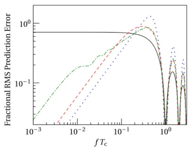
It may be helpful to visualise the spectral response of optim ised servos. Figure 2 shows, for a few simple cases, the RMS magnitude of the prediction error caused by a frequency modulation of the LO at some frequency f. In the absence of servo correction (black solid line), the response is lat at low frequencies but falls off as 1/f at high frequencies due to the averaging of the LO frequency within each interrogation cycle. Note that the servo prediction error vanishes at those frequencies to which the reference is insensitive: noise at these frequencies cannot be removed from the clock output, but it does not disturb the atomic reference and is therefore irrelevant as far as the servo is concerned. For a white-noise dominated system, the optimal controller has the lowest prac-tical gain, or equivalently averages as much history as is avail-able. The optimal spectral response function in this case looks essentially identical to the black line. For pure random-walk noise, which falls off rapidly at high frequencies, it is worth increasing the sensitivity to high-frequency noise in order to obtain better suppression at low frequencies: the optimal con-troller is then an integrator with a gain g=1.27 (blue dotted
line)5. The power spectral density of random-walk noise ∝ −
f 2
combines with the ∝f2 (power) response of an integrator to
yield a lat spectrum of contributions to the prediction error. In the intermediate case of licker noise, the same lat spec-trum could be achieved by a controller with a power response
∝f, i.e. an amplitude response ∝ f. The optimal 50-term
linear controller (green chain-dotted line) approximates this behaviour in the range of frequencies it can observe, from roughly 1 100/( Tc) up to 1 2/( Tc). At very low frequencies,
corre-sponding to luctuations slower than the 50-cycle memory of the controller, the response falls back to that of an integrator. A simple integrator cannot have a f amplitude response, so the best integrator for pure licker noise (red dashed line) is more sensitive to luctuations with periods of a few cycles. As a result it performs about 5% worse than the more general linear predictor.
To gauge their impact on clock performance, we quantify the scale of the servo’s prediction errors by the dimensionless variance
ω
= −
v ((x h) T)2
(12) of the phase accumulated in the Ramsey interrogation of dura-tion T. The variance v plays an important role in determining both the robustness of the lock to atomic resonance and the achievable long-term stability (see section 4), so that it is worth studying its behaviour. The solid lines in igure 3 illus-trate the performance of linear predictors, based on simula-tions of clock operation with between 1 and 104 atoms in the
reference. As a function of the choice of probe time T Z/ , and thus of the ratio between LO noise and measurement noise, one can distinguish three qualitatively different regimes. In the limit of large atom numbers and long probe times, the simulations approach an N-independent limit
⎜ ⎟ ⎛ ⎝ ⎞ ⎠ ξ = µ + v T Z . 2 (13)
This is the scaling one expects for the case where the LO noise completely dominates the measurement noise of the refer-ence, given the postulated power-law scaling of the LO noise with exponent µ (see section 1) and the deinition of Z in
equa-tion (3). The proportionality constant ξ can be estimated from the simulations or derived using the formulae in appendix A, and varies between 1 (for a white-noise- dominated LO) and 2 (for a random-walk-noise-dominated LO). In the opposite limit of low atom number or short probe time, the (white) quantum projection noise dominates and the servo perfor-mance depends only on the number of measurements n which it averages in making its prediction, and thus
Figure 2. Servo response spectra, expressed as the RMS prediction error caused by a unit-amplitude frequency modulation of the LO at frequency f, assuming a noiseless reference. Black solid line: no servo (open-loop). Dotted blue line: optimal linear predictor for pure random-walk noise (integrator of gain g=1.27). Chain-dotted green line: linear predictor optimised for pure licker-frequency noise, with a 50-cycle memory. Dashed red line: best integrator for pure licker-frequency noise (g=0.7).
5 Note that a random-walk-dominated system can require an integrator gain greater than unity. If, for instance, the last measured frequency was higher than the corresponding prediction, it is likely that the LO frequency was random-walking upwards during the last measurement, and thus that the frequency at the end of the measurement was higher than the average frequency during the measurement. The apparent over-correction implied by
>
g 1 is accounting for this difference. The integrating servo is still stable as long as g<2.
312 ≈ v Nn 1 (14) for suficiently short probe times. For n≳20 this limit has no impact on correctly optimised clock operation (see section 5). Between the two limits considered above there is a trade-off between averaging many measurements to reduce the impact of measurement noise and considering only the recent measure-ments most relevant to the LO’s current frequency. We know of no simple, accurate expression for the achievable servo perfor-mance in this intermediate regime, but the rough scaling that one would expect from the aforementioned trade-off
⎜ ⎟ ⎛ ⎝ ⎞ ⎠ ∝ µ + v N T Z 1 1 /2 (15)
does hold in simulations.
So far, we have discussed the simple integrator and its gen-eralisations. Practical frequency standards, however, must use a double-integrator to correct for steady drifts in the LO fre-quency [15]. With the addition of the second integrator, the servo predictions become
∑
= + + h h ge g e k k 0 1 1 2 (16) or∑
∑
= w y +g e . k k k k k 2 (17) Aside from its role in suppressing steady-state frequency errors with drifting LOs, the second integrator is necessary for the servo to have enough low-frequency gain to attain the projec-tion noise limit in many-atom clocks, a point to which we will return in section 7. However, as long as its gain g2 is chosen lowenough to avoid servo oscillations, the additional integrator has only a negligible impact on the variance of the prediction errors6. The controller can thus be designed by optimising a simple inte-grator or linear predictor as discussed above, and then adding the drift-correction integrator with a gain g ≪w =g
2 1 .
Besides minimising prediction variance, another desirable feature in practical servo controllers is robustness, the quality of remaining locked to the (correct) atomic resonance for long periods. In principle the two qualities are distinct, but we ind empirically that for well-optimised servos they are tightly cou-pled. In simulations of clocks with a wide range of atom num-bers (i.e. reference signal-to-noise ratios), we ind that the rate at which a clock hops to different Ramsey fringes depends, for a given LO and a fully optimised servo, only on the prediction variance v. Suboptimal servos (such as integrators with incor-rectly chosen gain) have both greater prediction variance v and a higher rate of fringe hops for a given v, so that they are less robust as well as noisier. We conjecture that the best servos are simultaneously the most robust and the least noisy, so that there is no need to choose between the two qualities provided that one can, in fact, ind this optimal servo design.
3. On-line servo optimisation and noise characterisation
In practice, the noise spectrum of the LO may not be known accurately. A signiicant beneit of the formalism presented in the previous section is that it allows one to optimise the servo controller without prior knowledge of the LO noise properties. This is possible because the deinition of C in equation (10)
involves only the estimated LO frequency error in each clock cycle, which is routinely recorded in normal clock operation7.
Figure 3. Variance of servo prediction errors, expressed as the variance v of the phase accumulated in a Ramsey interrogation, as a function of probe time for a white-noise (top) licker- (middle) or random-walk-limited (bottom) LO. The simulated clocks run for
×
2 106 Ramsey interrogations of 1 (solid black circles), 10 (open blue circles), 102 (solid red triangles), 103 (open green triangles)
or 104 (solid grey squares) uncorrelated atoms. Symbols show the
performance of integrating controllers optimised without knowledge of the LO noise as discussed in section 3. Solid lines show the performance of linear predictors using the last n = 50 frequency estimates, designed with knowledge of the LO noise properties as discussed in section 2.
6 This is best understood by considering the action of the servo in the fre-quency domain: the variance of the prediction errors depends on the feedback gain at a frequency corresponding to the clock cycle rate, whereas the second integrator only contributes feedback gain at much lower frequencies. The effect of the second servo is visible in the correlations between prediction errors, not in their variance.
7 In some implementations, the estimated frequency might not be recorded as such, but it can be obtained by adding the servo predictions to the frequency error signal reported by the atomic reference.
As a demonstration of such optimisation, we have run clock simulations with integrating servos whose gains were chosen, without knowledge of the true LO noise, by the following empirical procedure:
1. Start by setting the gain to g=0.2, an arbitrary but reasonable initial value chosen to allow reliable, if subop-timal, clock operation under a wide range of conditions. 2. Simulate the clock for 104 cycles, corresponding to a few
hours of operation for a typical contemporary frequency standard.
3. Compute C according to equation (10) and thence the
vector w of optimal weights. Set g = w18.
4. Simulate the clock with the newly optimised servo and reoptimise, repeating as necessary.
Even when the servo gain is initially chosen blindly, we ind that ive rounds of optimisation sufice for the gain g to conv-erge to a value that yields performance indistinguishable from that of an integrator designed with full knowledge of the LO noise spectrum. Under more realistic conditions, where the initial choice of servo parameters relects some prior knowl-edge of the LO performance, the optimisation could be per-formed much more quickly. The symbols in igure 3 show the prediction variance of such empirically-optimised integrators, which can be compared to the performance of optimal linear predictors shown as solid lines. For clocks operated near their optimal probe times (to be discussed in section 4), the differ-ence in prediction variance is less than 10%. Thus, it is pos-sible to develop controllers that take full advantage of the time correlations in the LO noise even without independent knowl-edge of those correlations.
Unfortunately, it is not always possible to verify the servo performance directly, because the observed variance of the error signal e contains contributions both from the servo pre-diction error and from measurement noise of the reference. For a single-atom clock this problem is insurmountable: the observed luctuations of a binary error signal must correspond to quantum projection noise, independent of servo perfor-mance. For a many-atom clock where the detection noise is well-characterised it is possible to measure the servo predic-tion variance as an increase in the luctuapredic-tions of the error signal, but the resulting estimates are generally optimistic. As discussed in section 4, even in a correctly optimised clock there will be unavoidable ambiguities in interpreting the error signal (e.g. 2π phase slips in Ramsey interrogation) and the
resulting measurement errors contribute to the servo predic-tion variance without being observable in the experimentally recorded measurement data.
One can, however, use the correlation matrix C estimated
during clock operation to partially characterise the LO. Although white noise of the LO is indistinguishable from measurement noise in the atomic reference, licker or random-walk noise can produce detectable temporal correlations even
when their contributions to the total measurement variance are small. By itting the estimated C to a linear combination
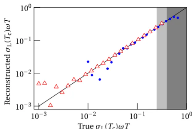
σ σ σ = + + C w2T C C T C c w f 2 f r2 c r ( ) ( ) (18) of the correlation matrices expected for white, licker and random-walk noise, one can obtain estimates of the Allan variances associated with each class of noise process, which are simply the coeficients in the linear combination. Explicit expressions for the correlation matrices associated with arbi-trary noise spectra are provided in appendix A. Figure 4, for instance, shows the licker and random-walk Allan devia-tions reconstructed in this fashion from a correlation matrix
C estimated from 2×10⁶ cycles of operation of a simulated
single-atom clock, normalised to quantum projection noise, as a function of the true level of the respective noise processes. Random-walk noise, whose correlations differ more strongly from those of the white measurement noise, is easier to detect, but as seen in igure 4 both licker and random walk noise can be reliably estimated from levels too low to affect the clock’s instability (variance less than 1% of projection noise) up to levels that would be unacceptably high in normal operation, when the clock servo is jumping between Ramsey fringes. Although this method provides much less detailed informa-tion on the LO noise spectrum than does the optical spectrum analyser of [34], it requires no measurements beyond those performed as part of the clock’s normal operation. It can therefore be used to monitor the LO while the clock is run-ning, even in a single-ion frequency standard, providing an early warning of performance degradations as well as infor-mation useful for the optimisation of interrogation parameters in the atomic reference (see section 5).
4. Impact of servo performance on long-term stability
Any measurement performed on a inite number of atoms can yield only a inite number of possible results. The optim isation of the measurement protocol thus involves a compromise
Figure 4. Normalised Allan deviation of licker (blue circles) or random-walk (red triangles) LO noise reconstructed from correlations in the error signal of a single-atom clock as a function of the actual noise level. Black line marks correct reconstruction. Light and dark grey regions mark the noise levels at which the clock servo hops between Ramsey fringes for random walk and licker noise respectively.
8 In cases where the noise is nearly white, this can lead to a theoretically optimal but practically useless controller with near-zero gain. To avoid this problem, we impose a minimum gain of 0.04 to ensure a inite servo attack time. This bound is low enough that it does not affect the achievable clock stability.
314
between ine resolution over a narrow usable domain of LO frequencies and coarse frequency resolution over a broader domain. The best compromise depends on the range of fre-quencies which might plausibly have to be measured by the reference, i.e. on the variance of servo prediction errors. In this section we study this compromise, showing that it leads to a inite optimal probe time and an overall limit on the long-term stability of clocks with noisy LOs.
By way of illustration, consider Ramsey interrogation of a single atom, where the probability to ind the atom in the excited state depends on the phase error φ=(x−h)ωT as
φ = + P 1 sin 2 . e (19)
This excitation spectrum is shown as a solid line of igure 5. Let us assume that, before any measurement, our best knowledge of the (corrected) LO frequency is represented by the chain-dotted distribution, corresponding to the distribution of LO prediction errors. Our best knowledge after a measurement on a single atom, in the event that it is found in the excited state, is shown by the dashed probability distribution. In this case we can be certain that the phase was not near φ= −π/2 (since the excitation probability would then have been 0), and we can be reasonably conident that it lies in the region between 0 and π, but we cannot rule out that it lies near −π, where both the
exci-tation probability and the prior probability distribution are non-negligible. Varying the probe time, and hence the spacing of the Ramsey fringes, involves a trade-off: increasing T narrows the main lobe of the posterior distribution, thanks to the steeper slope of the excitation signal, but also increases the weight of secondary lobes due to other fringes of the Ramsey spectrum.
To quantify this trade-off more formally, we consider Ramsey interrogation of N uncorrelated atoms, taking the prior distribution (chain-dotted curve in igure 5) to be a Gaussian of variance v φ π = −φ P v e 2 . v 2 2 ( ) (20)
This distribution encodes, formally, all that is known about the LO frequency before the atomic measurement result becomes available. In a practical sense, it is the distribution of servo prediction errors: if the servo prediction were perfect (h=x) then the phase accumulated in the Ramsey interroga-tion would be zero. The ansatz of equainterroga-tion (20) thus amounts to an assumption that the servo prediction errors are normally distributed. Although our simulations show some small devia-tions from the normal distribution, amounting to a negative excess kurtosis of a few percent with a single-atom reference that produces a binary error signal, the Gaussian ansatz is a surprisingly good approximation. As we will see, it leads to simple analytical results which agree well with more detailed simulations.
The reference does not, unfortunately, supply us with the expectation value Pe. Rather, the measurement yields a random
fraction F of atoms detected in the excited state that luctuates about the expectation value Pe due to measurement noise of
the atomic reference. In the absence of technical noise on the reference signal, the variance of F is
= − + − F P P P P N var( ) ( e ⟨ ⟩)e 2 e1 e ( ) (21) = + − − − v v N e sinh 4 1 e sinh 4 v v (22)
where the averages ⟨ ⟩⋅ are taken over the prior distribution φ
P( ). The irst term expresses the luctuations in the measured excitation fraction due to actual changes in the φ-dependent excitation probability, while the second corresponds to quantum projection noise of the binomially-distributed exci-tation signal. The usefulness of the exciexci-tation fraction in esti-mating the frequency depends on the covariance of the two quantities φ F = φF − φ F = v − cov , 2e v 2 ( ) ⟨ ⟩⟨ ⟩ (23) which determines how much weight should be given to F
in constructing the posterior estimate of the LO frequency. Choosing the weight to minimise the variance v′ of the error in this posterior estimate, we ind (see appendix C):
φ = − ′ v v F F cov , var 2 ( ) ( ) (24) ⎛ ⎝ ⎜ ⎞ ⎠ ⎟ = − − + v Nv N v 1 1 sinh ev . ( ) (25)
This posterior variance combines information from the mea-surement with information that was known beforehand. In order to isolate the contribution of the former, we deine an effective measurement variance vm by
= + ′ v v v 1 1 1 . m (26)
Figure 5. Schematic illustration of information gain in a single cycle of clock operation. Blue chain-dotted Gaussian: prior knowledge of the LO frequency. Black solid sinusoid: Ramsey excitation spectrum. Red dashed line: posterior knowledge of the LO frequency given that an atom was detected in the excited state. If no excitation is detected, then the posterior distribution is the mirror image about φ =0 of the one shown here.
This is the usual relation for the variance of a (posterior) estimate obtained by an optimal linear combination of two
independent pieces of information. vm is thus the variance of
a hypothetical measurement, one that could be interpreted without any prior knowledge, and which would reduce our uncertainty on the LO frequency as much as did the actual measurement. For the case we consider,
⎜ ⎟ ⎛ ⎝ ⎞ ⎠ = + − − v N N v v e 1 1 sinh v m (27) ⋯ ≈ + + + N v N v 1 2 6 2 3 (28)
where, in the second line, we have expanded the effective measurement variance in powers of the prior variance. The irst term is the conventional QPN on the measurement of the phase, valid when v is small and the corrected LO frequency is known a priori to be well centred on the Ramsey fringe. The third term relects the additional uncertainty arising when the corrected LO frequency can lie outside the range where the reference produces a meaningful result. This term is independent of atom number, and dominates the effective measurement variance as v approaches 1.
Replacing the standard phase variance of equation (1) by the effective measurement variance in equation (2) yields a new prediction for clock stability in the limit of large aver-aging time τ, one that accounts for the effects of limited prior information in each interrogation:
⎜ ⎟ ⎛ ⎝ ⎞ ⎠ σ τ ωT τ + − − T N N v v 1 e 1 1 sinh . v C( ) → c (29)
To demonstrate the validity of the simplifying approximations made in our model, such as the Gaussian ansatz for the dis-tribution of servo errors, we compare the zero-free-parameter prediction of equation (29) (igure 6, solid lines) to the stability of clocks simulated without making those approximations (igure 6, symbols). Clocks with white-, licker-, and random-walk-noise-limited LOs were simulated using Ramsey inter-rogation of uncorrelated atoms with no dead time (Tc=T).
Each point in igure 6 is obtained from a simulation of 2×10⁶
cycles of clock operation. The Allan deviation is computed for a time τ long enough that the instability has reached the asymptotic 1/ τ regime (corresponding to 2×10⁴ cycles of
clock operation), then rescaled to a ixed averaging time Z and normalised to a ixed noise level σ ZL( ) to obtain a
dimension-less result that is comparable across systems. The graphs thus show the achievable long-term instability as a function of the choice of probe time.
When the probe time is short, the Ramsey fringe is broad and v is small, the instability improves as 1/ T as conven-tionally expected. The improvement with increasing probe time stops either when the additional v-dependent terms in equation (29) grow important or when the servo can no longer reliably lock the LO to the reference transition: the curves in igure 6 end when the fringe-hop rate reaches 1 per 2 million cycles. As N increases, quantum projection noise is reduced relative to LO noise and it becomes advantageous to reduce
the probe time so as to be less sensitive to the latter. Thus, the optimal probe time gets shorter with increasing atom number, and the fully optimised clock instability does not scale as
N−1/2. The asymptotic scaling with N is given in table 1. For
white noise, the most extreme case, the optimal probe time scales as N−1/3 in the large-N limit, leading to a N−1/3 scaling
of the long-term Allan deviation. For licker or random-walk noise, v falls off more steeply as the probe time is shortened (see equation (13), so that the the optimal probe time is less sensitive to atom number and a scaling closer to the conven-tional QPN limit is obtained. In the absence of projection noise, i.e. in the limit N →∞, the servo performance limit of
equation (13) combines with equation (29) to yield a general measurement-noise-independent limit on clock instability, which we plot as dashed lines in igure 6. This limit arises solely from the unpredictability of the LO noise and from the inite domain over which the Ramsey error signal can be unambiguously interpreted.
Figure 6. Long-term instability as a function of probe time for clocks using Ramsey interrogation of 1 (solid black circles), 10 (open blue circles), 102 (solid red triangles), 103 (open green
triangles) or 104 (solid grey squares) uncorrelated atoms. Solid
lines show the prediction of equation (29), without free parameters. Vertical bars mark the recommended interrogation time given in table 2. Dashed line marks the limit for perfect phase estimation with no projection noise. The three graphs are, from top to bottom, for a white-, licker-, or random-walk-dominated LO. Simulations ran for 2×10⁶ clock cycles.
316
Strictly speaking, equation (24) holds only if the estimated frequency error is a linear function of the measured excitation fraction. Since the excitation probability is a non-linear (e.g. sinusoidal) function of the LO frequency error, one might hope to do better than the estimated performance of equation (29) by using a non-linear function to convert the excitation frac-tion to a frequency error estimate. Simulafrac-tions show, however, that correcting for the curvature of the Ramsey fringe by esti-mating the accumulated phase as arcsin 2( F−1) rather than
simply 2F−1 has no signiicant effect on v or on the
achiev-able long-term clock stability. One can understand this inding by noting that, when v is large enough that the curvature within a single Ramsey fringe is signiicant, the effect of unavoidable ambiguities such as the secondary lobe in igure 5 is much larger and dominates the posterior variance.
5. Guidelines for interrogation parameters
To choose the operating parameters for a clock, one can in general use the formalism of section 2 to predict the servo error variance v as a function of those operating parameters and equation (29) to predict the resulting long-term stability, which can then be optimised. Table 2, for example, provides recommended Ramsey interrogation times for clocks domi-nated by different types of power-law LO noise, expressed as multiples of Z. In the many-atom limit, the servo prediction errors become independent of the quantum projection noise and we can solve equation (29) to obtain the asymptotically optimal probe time (last column of table 2). Increasing the probe time beyond this optimum always leads to an increase in effective measurement variance and long-term instability, and is of no practical interest. At small atom numbers, shorter probe times are required to keep the servo controller robust against fringe hops. The purely phenomenological bound in the second column of table 2 is chosen to be slightly shorter than the time for which we observe fringe-hops at a rate of 1 per million simulated clock cycles, with a 20% safety margin. Our choice of maximum acceptable fringe-hop rate, corre-sponding to a requirement that the clock remain locked to the correct fringe for a few days, is arbitrary, but as the onset of fringe-hopping is extremely steep (the fringe-hop rate in sim-ulations increases by two to three orders of magnitude when the probe time is doubled), the maximum safe probe time is only weakly dependent on this choice of threshold. A full optim isation of all common probe protocols in the presence of realistic experimental imperfections is beyond the scope of this work, but we expect qualitatively similar behaviour
from Rabi or hyper-Ramsey probing, with somewhat longer optimal probe times and slightly degraded instability due to the increased width of the observed atomic resonance in theses schemes. Conversely, we expect that clocks with signiicant dead time in their operating cycle will need to use somewhat shorter probe times to compensate for the servo’s inability to correct unobserved LO frequency luctuations, which will lead to a v higher than in our dead-time-free simulations.
6. Constraints on the beneits of entangled atomic references
The arguments developed in the preceding sections also apply to certain Ramsey-like protocols using entangled states in the atomic reference, provided that LO noise is the limiting form of decoherence. For instance, the scheme proposed in [35] and demonstrated in [36–38], employing N atoms in a maximally correlated state (|ψ⟩= |( ⟩g⊗N+|e⟩⊗N)/ 2, where |g⟩ and
|e⟩ are the atomic eigenstates), is fully equivalent to Ramsey interrogation of a single atom with an N-fold enhanced trans-ition frequency by the corresponding harmonic of the LO radiation. Now the long-term instability of a single-atom fre-quency standard can be expressed as
σ τ ω τ = s Z , C( ) (30) with s a dimensionless constant of order unity encoding the choice of probe time T Z/ and the additional contribution of LO noise at this probe time. The long-term instability of the clock using maximally-correlated atoms thus becomes
σ τ ω τ = s N ZN , C( ) (31) where ZN is the noise timescale for the N-fold frequency-
multiplied LO:
σL(ZNc)N Zω N=1 rad.
(32) In the dead-time-free limit ZNc=ZN, one can compare
equations (32) with (3) and ind
= µ − + Z Z N , N 2 2 (33) with µ again describing the time-dependence of the LO Allan
variance (see section 1). The entangled clock’s long-term instability thus scales as
Table 2. Recommendations for the choice of Ramsey interrogation time. The last column gives the optimal probe time in the limit of many atoms. There is nothing to be gained by probing longer than this time. It may be necessary to use shorter probe times to avoid fringe hops; a suggested safe upper bound on the probe time is given in the second column.
LO noise Safe T Z/ Asymptotic optimum T Z/ White — min(N−1 5/, 1.4N−1 3/) Flicker 0.4−0.15N−1 3/ 0.76N−1 6/ Rnd. walk 0.4− − N 0.25 1 3/ − N 0.79 1 9/
Table 1. Asymptotic scaling of LO-limited clock instability with atom number. The scaling differs from the conventional N−1/2 QPN
limit because the optimum probe time decreases with increasing atom number. LO noise type Asymptotic scaling of σ τ ωC( ) Zτ White ∝ N−1/3 Flicker ∝ N−5/12 Rnd. walk ∝ N−4/9 Metrologia 54 (2017) 307
σ τ ω τ = µ µ + + s Z N 1 . C 1 2 ( ) (34)
Thus, if the clock stability is limited by white LO noise (µ = −1), a reference using a maximally-correlated state of
N atoms performs no better than a reference using a single
atom, and is in fact worse than a reference using uncorrelated interrogation of the N atoms. This scaling has been observed experimentally for correlated magnetic ield noise in a 14 ion GHZ state [38]. For licker-loor LO noise, the Allan deviation improves as N−1/2
with N maximally-entangled atoms, very slightly better than the asymptotic N−5/12
scaling achievable without entanglement, but worse than the scaling achieved with unentangled atoms for N < 102. It is only for
random-walk LO noise that maximally entangled states offer measur-able beneits, with an N−2/3
scaling of the long-term Allan deviation. We illustrate these scalings in igure 7, which plots the Allan deviation spectrum recorded in simulations of fully
optimised clocks using either 100 uncorrelated atoms or a 100-atom maximally-correlated state for all three LO noise types.
Maximally entangled states reduce the signal-to-noise ratio of a measurement on N atoms to that of a single qubit, pro-viding less new information per measurement but accelerating the clock cycle so that more measurements can be averaged. That is why their use is advantageous with random-walk LO noise, when fast measurements can take advantage of the reduced LO noise at short time scales. Other approaches to the use of entanglement in atomic references, such as spin squeezing [24–26, 39–41], focus instead on improving the signal-to-noise ratio of the measurement, and thus increasing the amount of new information obtained in each interroga-tion. The error signal produced in such schemes has the same periodic ambiguities as in Ramsey interrogation of uncorre-lated atoms, and so they are subject to the same projection-noise-independent sinhv−v≈v3/6 limit on their effective
measurement variance (see equation (28). The additional noise introduced when servo prediction errors allow the anti-squeezed quadrature to contaminate the measurement result [42] can in principle be eliminated by a suitable readout pro-cedure [27] in which case we expect such interrogation proto-cols to offer beneits comparable to suppressing the projection noise by increasing atom number, even with white- or licker-loor limited LOs.
7. Some remarks on short-term instability
So far we have focused on the long-term instability of the clock once it reaches the asymptotic σC∝1/ τ regime,
without considering the averaging time required to reach this regime. In general, a clock reaches its asymptotic instability when the luctuations in the frequency of the output signal are dominated by the measurement noise of the atomic reference. For single-ion clocks in which the signal-to-noise ratio of the atomic measurements is no better than 1, this condition is reached at the servo attack time τ1, as soon as the output signal
of the clock stops following the free-running LO and is locked to the noisy signal from the atomic reference. However, clocks using many atoms have a much higher signal-to-noise ratio, i.e. the resolution of the error signal from their atomic refer-ence is much iner than the LO frequency luctuations that they can reliably measure. In such clocks the optimal probe times are long enough that the quantum projection noise is well below the LO-limited short-term instability. In order to reach the asymptotic regime they must initially average down faster than 1/ τ. This is possible provided that the servo has enough
gain to suppress the measured LO frequency luctuations. A single integrator can suppress measured LO luctuations by a factor ∼τ τ/1 in the standard deviation9, so that the clock
instability initially averages down as τ−3 2/ or τ−1 for white
or licker LO noise respectively. This is fast enough to reach the measurement-noise limited regime in an averaging time of roughly Nτ1 or Nτ1 for a white-noise-limited or licker-loor
Figure 7. Simulated Allan deviation as a function of averaging time for optimised clocks using either 100 uncorrelated atoms (solid blue circles) or a maximally-correlated state of 100 atoms (open red circles). The latter must operate with shorter interrogation times, and thus the corresponding curves start earlier. The black line marks the Allan deviation of the free-running LO. The three graphs are, from top to bottom, for a white-, licker-, or random-walk-dominated LO. Arrows mark the two integrator time constants for the case of uncorrelated atoms, as discussed in section 7.
9 This is the time-domain equivalent of the observation that an integrating servo suppresses noise power at a frequency f by a factor proportional to f 2.
318
limited LO respectively, as seen in the irst two graphs of igure 7. However, a single integrator can only suppress random-walk LO noise to a level that scales as τ−1 2/ , which
will not catch up with the measurement noise limit which is averaging down at the same rate. A many-atom clock using only a single integrator would thus be forever limited by the inite gain of the servo rather than by the noise of the atomic measurements. It is only when a second integrator allows the servo to suppress noise by an additional factor of τ τ/ 2 that the
clock instability can average down as τ−3 2/ until it reaches
the measurement noise limit in a time Nτ2. The third graph
of igure 7 illustrates this behaviour, with the uncorrelated 100-atom clock initially averaging down at the servo-limited rate of τ−1 2/ until around τ ≈2 45Z. The second integrator
then allows the instability to catch up with the lower-lying asymptotic noise limit, which it reaches around τ ≈400Z. It
is interesting to note that clocks using maximally-correlated states, because they behave like single-atom clocks and are always measurement-noise limited, would have an advantage in short-term instability even when their long-term instability is little better than that of a clock with uncorrelated atoms (lower two graphs of igure 7). This observation mirrors, in a simpler setting, the inding of [20].
Thus the second integrator in a clock servo, beyond its role in correcting for linear drifts, is also needed to suppress random-walk noise of the LO in many-atom clocks. It is desirable to set the gain g2 of this drift-correction integrator
as high as possible, in order to reach the asymptotic insta-bility in a reasonable time. However, it must not be so high that it induces oscillations in the lock. With a conventional two-stage integrating servo, the ratio of the two gains must be no more than a few percent (we use g2 = g/50 in our
simula-tions). Linear predictors optimised as in section 2 are some-what more robust against oscillations, and can be operated with higher gain g2=w 101/ for the drift-correction integrator.
When post-processing measurement results to generate a virtual ‘paper’ clock signal, the causality requirements which limit the gain of the servo during physical clock operation no longer apply. Thus, while the long-term stability limits dis-cussed in section 4 hold equally for physical and paper clocks because they arise from limits on the noise of the atomic ref-erence, the short-term stability limits discussed in this sec-tion can be avoided entirely in paper clocks and frequency ratio measurements, where the LO frequency luctuations can always be corrected as well as they can be measured.
More abstractly, this section can also be understood in terms of the difference between steering the clock’s frequency and steering its accumulated phase (i.e. indicated time). The asymptotic limit of equation (29) corresponds to an unavoid-able random walk of phase due to the undetectunavoid-able and uncor-related frequency measurement errors of the atomic reference. To reach it, one must irst correct the clock’s output for all the detected LO frequency errors, which dominate the short-term instability in multi-atom clocks. Within our model this is done by the servo, the only component of the system with memory, and thus the only component capable of remem-bering and correcting past phase errors: an Allan deviation averaging down faster than 1/ τ indicates that the servo is
steering phase rather than simply locking frequency. This can happen only slowly, however, as it must not interfere with the servo’s primary task of keeping the LO frequency near atomic resonance so that the reference continues to yield informa-tive measurement results. In clocks where separate correc-tions are applied to the output signal and to the signal used for atomic interrogation, the latter can be kept on resonance while the former’s phase is corrected as fast as possible (even pre- emptively in the case of a paper clock), thus minimising short-term luctuations in the timing error.
8. Outlook
In this work we have studied the effects of LO noise on fre-quency standards that monitor the LO frefre-quency using a single ensemble of atoms periodically interrogated according to a ixed protocol and that correct the measured frequency luctu-ations using a linear prediction formula. Most current optical atomic clocks it this description and can, without hardware modiications, use the framework presented here to identify and approach the stability limit imposed by their LO perfor-mance. The interrogation times we recommend are speciic to dead-time-free Ramsey interrogation, but qualitatively similar results for other (Rabi, hyper-Ramsey) protocols can be found by the same arguments, since our treatment of the servo is protocol-independent and since all interrogation protocols face the same trade-off between measurement resolution and unambiguous measurement domain. Within this framework, the most promising approaches to improving long-term clock instability (besides improving LO performance) seem to be those that improve the dynamic range of atomic measurements (such as spin squeezing), whereas methods which attempt to make faster measurements with poor dynamic range (such as spectroscopy with maximally-correlated states) have been shown to offer modest or no beneits for realistic LO noise spectra.
There are, however, many architectures for frequency standards that do not it the framework presented here, and it would be interesting to consider which of them can overcome the limits we have identiied. The simplest extension to imple-ment would be the use of non-linear prediction algorithms, which might improve the robustness of the servo, allowing longer probe times and better stability at small atom number. We expect that the performance of such algorithms would still be subject to the measurement-noise-independent limit of equation (13), so that they are unlikely to offer more than a modest constant-factor stability improvement in the large-N limit.
Proposed multi-ensemble or cascaded clocks [19, 20] cir-cumvent the limits we have discussed here by monitoring the LO noise with several different atomic references with pro-gressively iner resolution. References with a broad domain of useful frequencies provide coarse-resolution results suficient to narrow the prior v for other, iner-resolution references. The analysis we have presented here applies directly to the irst (coarsest) reference in the cascade, and the resulting stabilised signal can then be treated as an effective LO used by the next