Applications of reference cycle building and K-shape clustering for anomaly detection in the semiconductor manufacturing process

(1)

Applications of Reference Cycle Building and K-shape Clustering for Anomaly Detection in the Semiconductor Manufacturing Process

by

Han He

Master of Science in Mechanical Engineering University of Illinois at Urbana-Champaign, 2017

Submitted to the Department of Mechanical Engineering in fulfillment of the requirements for the degree of Master of Engineering in Advanced Manufacturing and Design

at the

MASSACHUSETTS INSTITUTE OF TECHNOLOGY

September 2018

The author hereby grants to MIT permission to reproduce and to distribute publicly paper and electronic copies of this thesis document in whole or in part in any medium now known or hereafter

created.

Author

Signature redacted

Department of Mechanical Engineering August 14, 2018

Certified by

Signature

redacted

Duane S. Bbg Clarence J. LeBel Professor, Electrical Engineering and Computer Science

Thesis Supervisor

Signature redacted

Certified by________________

David E. Hardt Ralph E. and Eloise F. Cross Professor, Mechanical Engineering Thesis Reader

Accepted by

Signature

redacted

MASSACHUSETTS INSTITUTE _RhnAeaan

OF TECHNOLOGY Rohan Abeyaratne

Quentin Berg Professor, Mechanical Engineering Chairman, Committee for Graduate Students

(2)

(3)

Applications of Reference Cycle Building and K-shape Clustering for Anomaly Detection in the Semiconductor Manufacturing Process

by Han He

Master of Science in Mechanical Engineering University of Illinois at Urbana-Champaign, 2017 Submitted to the Department of Mechanical Engineering

on August 14, 2018 in partial fulfillment of the requirements for the degree of Masters of Engineering in

Advanced Manufacturing and Design

Abstract

Early and accurate anomaly detection plays a key role in reducing costs and improving benefits, especially for complicated and time-consuming manufacturing such as semiconductor production. A case study of detecting anomalies from several monitored parameters during one plasma etching process is presented in this thesis. The thesis focuses on optimized ways to build reference cycles, or centroids of univariate parameters, a critical component to determine clustering accuracy and to facilitate process engineers' offline anomaly detections and diagnoses.

Three time series centroid building methods are discussed and evaluated in the thesis, arithmetic, the Dynamic Time Warping Barycenter Averaging (DBA), and the soft-DTW-based centroid. As a result, DBA is chosen considering its comprehensive performance of accuracy and calculation time. Optimizations on DBA is further discussed to reduce calculation time. The window constraint, as well as the recalculation method of combining the previous centroid and new datasets, substantially reduce calculation time with slight accuracy loss.

Based upon one centroid building method, shape extraction, a novel clustering method, k-shape, is implemented and applied to the plasma etching process. It is found that it achieves great accuracy with substantially shorter calculation time than one mainstream clustering method, k-means.

Thesis Supervisor: Duane S. Boning

Title: Clarence J. LeBel Professor, Electrical Engineering and Computer Science

Thesis Reader: David E. Hardt

(4)

(5)

Acknowledgements

I would like to take this opportunity to deliver my sincere appreciation to the people helping me in this project.

First I would like to thank MIT and ADI for providing such a challenging and meaningful joint project to practice my skills and expand my expertise. The experience I have learnt from this project will be a solid background for my future career.

Thanks to Mr. Jack Dillon for his tremendous and prompt coordination and assistance in this project. I feel so supported in ADI with his help. Thanks to Mr. Ken Flanders for sharing his insights and leading me to the theoretical world of the semiconductor industry. Thanks also to Mr. Leslie Green and Mr. Charles Mathy for their expertise and inspirations.

Thanks to Dr. Duane S. Boning for his patient and thorough instructions and guidance during the project. Without his encouragement, I cannot easily jump out of the traditional anomaly detection methods, apply and optimize a series of innovative methodologies in this project.

Thanks to Mr. Jose J. Pacheco and Dr. David E. Hardt for the great operation and organization of the MEng program during the past year. It is a fabulous experience enriching my life and memory.

Thanks to my teammates, Tiankai Chen and Oumaima Makhlouk, for your seamless cooperation and strong support during the project.

Finally, I would like to thank my parents for their consistent understanding. Thanks to all the people who are loving and kind to me. You make my life brighter than I think.

(6)

(7)

Table 6. Average Performance of Centroid Methods on the Parameter 'Bot_RF_RevPwr', with Arithmetic the D B A as Preset C entroid ... 49 Table 7. Average Performance of Window-constrained DBA on the Parameter 'BotRFRevPwr' ... 58 Table 8. Comparison between Recalculation M ethods... 59 Table 9. Derivatives of the Summed Square SBD vs. Quantity of Clusters for the k-shape Clustering .... 62

Table 10. Confusion Matrix of k-shape on the 341 'ProChm_EndPt_ChanC' Time Series ... 64

Table 11. Confusion Matrix of 3-Cluster k-means on the 341 'ProChm_EndPt_ChanC' Time Series...64 Table 12. Comparison of k-shape and k-means Performance on the 341 'ProChmEndPtChanC' Time

(10)

List of Figures

Figure 1. M achine H ealth Project Fram ework... 15

Figure 2. Schematic of Plasma Etching Process [6] ... 16

Figure 3. Plots for Parameter Behaviors for the Recipe 920, with Left the Good Cycles and Right the Bad C y c le s ... ₁₈

Figure 4. Mixture of Normal and Bad Time Series Data of Parameter 'ProcChmEndPtChanCIn'...20

Figure 5. O riginal vs. W insorized D ata [8]... 23

Figure 6. Mapping between the Two Time Series [9] ... 24

Figure 7. Resampling the Time Series according to Relative Indices ... 32

F igure 8. C onfusion M atrix ... ₃₃

Figure 9. G ood Cycles of 'BotRF _RevPwr' ... ₃₇

Figure 10. Good Cycles of 'ProChmEndPtChanC' ... 37

Figure 11.Time Series for Parameter 'Bot_RFRevPwr', with Sample Size of 20... 39

Figure 12. Time Series and Centroid for Parameter 'BotRFRevPwr', with Sample Size of 20 and DBA C entroid B uilding M ethod... ₄₀

Figure 13. Time Series and Centroid for Parameter 'BotRFRevPwr', with Sample Size of 20 and soft-DTW Centroid Building Method with y of 0.001 ... 40

Figure 14. Time Series and Centroid for Parameter 'Bot_RFRevPwr', with Sample Size of 20 and soft-DTW Centroid Building Method with y of 0.01 ... 41

Figure 15. Time Series and Centroid for Parameter 'Bot_RFRevPwr', with Sample Size of 20 and soft-DTW Centroid Building M ethod with y of 0.1 ... 41

Figure 16. Time Series and Centroid for Parameter 'Bot_RFRevPwr', with Sample Size of 20 and soft-DTW Centroid Building Method with y of 1.0 ... 42

Figure 17. Time Series and Centroid for Parameter 'Bot_RFRevPwr', with Sample Size of 20 and A rithm etic W insorization M ethod... ₄₂

Figure 18. Time Series and Centroid for Parameter 'Bot_RERevPwr', with Sample Size of 20 and Arithm etic Untrimm ed M ean M ethod... ₄₃

Figure 19. Time Series and Centroid for Parameter 'Bot RFRevPwr', with Sample Size of 20 and A rithm etic M edian M ethod ... ₄₃

(11)

Figure 21. Improvement on the Time with Preset Centroids for Soft-DTW...51

Figure 22. Improvement on the Mean SBD with Preset Centroids for Soft-DTW ... 52

Figure 23. Improvement on the DTW Distance with Preset Centroids for the DBA Method ... 54

Figure 24. Improvement on the Time with Preset Centroids for the DBA Method ... 54

Figure 25. The Window-Constrained Warping Path, with Red Elements not Considered in the DTW[7].56 Figure 26. Mean DTW Distance Increase for the Window-Constrained DBA... 57

Figure 27. Time Reduction for the W indow-constrained DBA ... 57

Figure 28. Mixture of 341 'ProChm_EndPt_ChanC' Time Series Data...60

Figure 29. Summed Square SBD vs. Quantity of Clusters for the k-shape Clustering ... 61

Figure 30. Result of the 4-cluster k-shape Clustering on the 341 'ProChm_EndPt_ChanC' Time Series .62 Figure 31. Result of the 3-cluster k-means Clustering on the 341 'ProChm_EndPt_ChanC' Time Series63

(12)

1. Introduction

This introduction describes the value and the objective of the Machine Health Project from the level of ADI and the research team, then introduces individual tasks, and finally outlines the organization of the thesis.

1.1 Project Overview

Analog Devices Inc. (ADI) is an American international semiconductor company, specializing in the design, manufacture, and marketing of high performance analog, mixed-signal, and digital signal processing integrated circuits. The company's products play a fundamental role in converting, conditioning, and processing real-world phenomena such as temperature, pressure, sound, light, speed, and motion into electrical signals to be used in a wide array of electronic devices (Inc., 2015)[1]. Its products have been widely used in instrumentation, automation, communications, healthcare, automotive and numerous other industries [2].

In view of the fabrication cost, ADI faces the cost pressure to optimize manufacturing systems and processes, and is therefore exploring new approaches including machine learning to improve manufacturing. Before chips are finally diced, packaged and shipped, each wafer has to go through multiple process cycles such as plasma etching and implantation. Overall the process is long and suffers from low yield. Commonly when one certain cycle goes wrong, it is hardly possible to detect the anomaly in time and hence the entire process continues until the entire process is finished, at which point wafers may be found defective at the end. Such process failures during the production cause losses in both production costs and time, which are significant for the capital-intensive semiconductor industry. If anomalies could be detected in earlier and accurately, the

(13)

plant could either scrap the work-in-progress part or adjust the following processes accordingly to compensate for the loss. Therefore it is meaningful to explore expanded monitoring of the process parameters, and accurately alarm and notify operators in time so that they can respond to anomalies at an early stage. ADI is thus interested in such in-time anomaly detections and gets involved in a series of innovative projects.

One such project is the Machine Health Project. The project intends to improve the way ADI collects and analyzes the data from the process. Its objective is to monitor process parameters, provide timely alerts on anomalies and thus enable efficient and effective response in time. It seeks improvements on machine reliability, productivity, quality and cost. In addition to the traditional methods such as traditional Statistical Process Control (SPC), ADI is seeking the feasibility of applying advanced methods such as machine learning to their production systems for further improvements.

1.2 Project Scope

Our project is to optimize the health monitoring model for machines and processes in ADI's Wilmington Fabrication Plant. Our team consists of three MIT students engaged in thesis research as part of the Master of Engineering in Advanced Manufacturing and Design Program. The objective is to evaluate the appropriate analytic techniques for timely anomaly detection.

The project requires us to implement analytics using R within the SQL server, which needs careful and efficient data preprocessing. ADI expects some "real-time" analytic tools and best practices, which could be either integrated into the online analytic platform or be provided to process engineers for their daily and off-line work.

(14)

The objective of the project includes:

" Evaluate key parameters and methods for anomaly classification " Evaluate methodologies and algorithms for timely anomaly detections * Find solutions to anomaly detection methodologies and algorithms * Determine best practices for implementing "real-time" analysis

" Provide efficient and useful assistance tools for process engineer's daily analysis

According to the objective, the framework of the Machine Health Project is summarized in Figure 1. The data received from the machine's sensors is first preprocessed in the pre-processing section. The preprocessed data can be presented in plots by the visualization section. Then the pre-processed data goes through the data analytics section. The data be captured as reference cycles, or can go through the anomaly detection part. The built reference cycles in turn facilitate anomaly detection. Results of both reference cycle and anomaly detection can be shown in plots by the visualization section. After the data analytics section, the result goes through the interface section. The anomaly is alerted to the process engineers and all results and records are sent back to the database. Through the improvement of anomaly detection, the plant gains multidimensionally in terms of cost, yield and machine life. The algorithms themselves are not process, recipe and machine dependent, so that they could be extensively applied conveniently.

(15)

Data Analytics Database Pre-Processing-Reference Anomaly Cycle Detection Visualization -- Interface

Figure 1. Machine Health Project Framework

1.3 Problem Statement

The problem statement explains the part of the project this thesis focuses on. The major case the team has worked on is first presented, and then the specific individual task to be solved in this thesis is described.

1.3.1 Case Overview

The major case studied in the project is related to unconfined plasma excursions happening during the plasma etching process. Plasma etching is one major process of semiconductor production. It involves plasma of an appropriate gas mixture generated and exposed to a sample. The plasma consists of etch species, which are either charged or neutral. The charged species are composed of ions and the neutral consist of atoms and radicals. During the process, the reactive species produced by the plasma react with the materials to be etched and produce volatile etch

(16)

products at room temperature. Finally, the charged species are accelerated vertically to the wafer substrate by the applied electric field and embed themselves at or just below the target surface. In this way the target's physical properties are modified [5]. The mechanism is shown in Figure 2.

PLASMA

ions

neutrals

electric field

photomask

substrate

Figure 2. Schematic of Plasma Etching Process [6]

The unconfined plasma excursion causes unplanned etching on the wafer. Currently for the machine 'OXLR7_LAMALl' three major related parameters are monitored and analyzed: 'BOTRFRevPwrIn', 'ProcChmBotElecTempMon' and 'ProcChmEndPtChanCIn'. These parameters come with respectively definitions and meanings:

BOTRFRevPwrIn: The amount of the reflected Radio Frequency (RF) power reflected back to the supply. Radio Frequency (RF) power is used in plasma etching to ionize the gas generating a plasma. The RF power is a programmable parameter that is part of a recipe for the particular etch. Forward power is the power delivered to the load and reflected power is the power that is reflected back to the supply. Ideally reflected power is 0 W. However, due to inefficiencies of the RF match

(17)

network or the physics of the chamber, there are losses. Reflected power is an indicator of how efficiently the power is being delivered to the chamber or the load.

ProcChmBotElecTempMon: An indicator of the temperature of the wafer during processing. The work-in-progress wafer sits on a chunk during processing with temperature monitored and recorded.

ProcChm_EndPtChanC_In: A parameter used to determine whether the etch is complete. It provides a signal, expressed in counts, of the plasma intensity at a specific wavelength. As the target material being etched is completed, the next layer is exposed, which results in a change in the spectrum along with a change in amplitude of the endpoint signal. A parameter value of zero indicates the completion of the etching.

Plots for each parameter are shown in Figure 3 for Recipe 920, with good-behaved cycles and mix-behaved cycles listed separately. A total of 341 cycles' data is shown in the figures.

Cyde - 20160804034344 s0 2e+05 30+05 2.0-C it I fi .5 --0.00

Oe+00 1e+05 2e+05 3e+05 Time - 20160604_034915 - 20160004_03S537 - 20160804.04011C - 20166604_040644E - 20160604_04122C - 20160604.123334 - 20160604_123905 - 20160604_12443e - 20160804_125012 - 20160804_125547 - 20160804_130121 - 20160004_13065t Cyde - 2016004_034344 - 20160604_034915 - 20160604.035537 - 20160004_04011C - 2016064_04064e - 20160904_04122C - 20160804_123334 - 20160004_12390! - 20160604124436 - 20160904.125012 - 20160604.125547 - 20160604.130121 - 20160604_13065C 60- 40- 20-00+00 1e+05

-1

Time 2e+05 3e+05 2 CL is I fi 'd Cyde - 20160725_10114e - 20160725_101721 - 20160725_102302 - 20160723_10237 - 20160725.10340M - 20160725_103939 - 2016072%_10451e - 2016072-_10505C - 20160725_105624 - 20160723.11015e - 2016072S.110733 - 20160725_111304 - 2016072%_11183E Cyde - 20160719_094214 - 20160719094747 - 20160719_095326 - 20160719_095902 - 20160719.1041 - 20160719_101015 - 20160719_101549 - 20160719_102121 - 2060719_102653 - 20160719.103227 20160719.103802 - 20160719.104335 - 20160719_104O09

00+00 1e+05 2e+05 3e+05

Time 60 - 020-0 -Oe+00 le+05 0

(18)

Cyde Cyde - 20160804_034344 - 20160725101148 8000 - 20160004_03491S 30000 - 20160725.101721 - 201600804035537 - 20160725_10230; - 20160804.04011C - 20160725.102837 r - 201608042040644 - 20160725103408 22010804.133C - 20160725.1053S -201609040124X-21075152 5000- - 20160004.123334 - 20160725101e E - 20180804.2390! 1 - 20160723SOX0S X- 20160904:2443E - 20160725.103624 'd 400w -A000 - - 2010804.125013 - 20160723..11015e -- 20160804125547 - 20160723_110733 - 2016004_1301231 - 20160723111304 0 - 20160804.13065f 0- - 20160725_11183e

0000 1e.05 2e+05 30+05 00+00 10+05 20+05 3e+05

Time Trne

Figure 3. Plots for Parameter Behaviors for the Recipe 920, with Left the Good Cycles and Right the Bad Cycles

As can be seen, parameters behave normally in a cycle within ranges of amplitude and phase. For the parameter 'BOTRFRevPwr_In', it can be seen that the major anomaly is a step increase in the power in the first 80% section of the cycle. For the parameter 'ProcChmBotElecTempMon', major anomalies are sudden and drastic increases and decreases in the temperature at turning points rather than smooth changes. For the parameter 'ProcChmEndPtChanCIn', the major anomaly is the much higher saturation point. Normally the value should be below 8000. In anomaly cases, the value reaches over 30,000 and stays at such high level until the end.

1.3.2 Individual Task

Individually, the initial objective in this thesis is to provide an accurate and efficient tool to assist engineers in building reference cycles, or centroids for their daily data comparison and analysis. Then, related and extensive applications of the centroids for anomaly detection and classification are explored, mainly around the k-shape clustering method.

(19)

When meeting with process engineers in ADI, we found that they preferred to manually track back anomalies using Excel. Normally, they plotted each process parameter and reasoned which parameter went wrong according to their experience, or rules of thumb. This method mainly caused two problems. Initially, without a standard centroid for each parameter quantitatively and geometrically in mind, engineers could easily incorrect false judgements and they tend not to make consistent judgements about the same cycle. This issue could be worse for engineers unfamiliar with the process.

In addition, without a mutually agreed-upon standard cycle, different engineers apply their individual rules of thumb and form diverse centroids in their minds. As a result, they sometimes cannot reach agreement on the anomaly detection for the same cycle. In short, currently process engineers cannot make consistent judgements on anomaly detection personally and interpersonally. One of the examples is the analysis of the parameter 'ProcChmEndPtChanC_In', with the data shown in Figure 4. Among the 11 cycles, the three low-amplitude cycles are correct. However, it is hard for engineers to describe the amplitude and shape of such a good cycle accurately and thus they tend to make mistakes in later anomaly detections and analysis. It is necessary to help engineers build accurate centroids from normal cycles. These cycles improve their anomaly detection accuracy and analysis quality when they work offline. With a mutually agreed-on centroid, it is also smoother and more efficient for engineers to reach agreement on anomaly detection results.

Furthermore, an accurate centroid also improves the quality of semi-/automatic anomaly classification and detection methods, such as clustering. In addition to providing practical and accurate centroid building tools for process engineers, extensive applications of the centroid in anomaly detection and classification are also explored in the thesis.

(20)

ProcChm_EndPt_ 35000 _ChanCIn 30000 25000 U 20000 C U 15000 10000 5000 0 queL

Figure 4. Mixture of Normal and Bad Time Series Data of Parameter 'ProcChm_EndPt_ChanC_In'

1.4 Thesis Outline

After the project's objectives and the problem statement are presented in Chapter 1, introductions to theory and algorithms are summarized in Chapter 2. These include the methods to measure the similarity between time series, centroid building methods, and one novel clustering method, the k-shape. Additional and necessary theories are introduced, such as the resampling for data pre-process, and the confusion matrix for clustering performance evaluation.

Following the discussion of theoretical background, methodologies for developing experiments evaluating diverse centroid building methods are discussed in Chapter 3. This chapter details the structure of experiments and important factors considered in designing experiments.

Results and discussions are presented in Chapter 4. The discussion is not only on the type of the centroid building method preferred, but also on optimization methods for further improvements. In addition, a brief evaluation of the k-shape clustering is presented. Finally, Chapter 5 makes conclusions on experiment results, value to ADI and recommendations on further tests and improvements.

(21)

2. Theoretical Backgrounds

Chapter 2 focuses on theoretical backgrounds the thesis is based on. Section.2.1 introduces metrics of judging time series similarities and types of centroid building methods. Section 2.2 introduces clustering theories and then the k-shape clustering method. Section 2.3 describes resampling, one necessary signal pre-process step. Finally, Section 2.4 introduces an important clustering evaluation method, the confusion matrix.

2.1 Time Series Similarity Measurement and Centroid Building Methods

This section first introduces a fast but inaccurate way to calculate centroids, the arithmetic method. In view of the arithmetic method's inaccuracy, metrics to evaluate time series similarities and build centroids are then introduced. One quantitative metric measuring the distance, Dynamic Time Warping (DTW) distance, is introduced in Section 2.1.2. The centroid building method based upon DTW distance, DTW Barycenter Averaging (DBA), along with a variant of DTW, soft-DTW, and the centroid building method based upon soft-soft-DTW, are each presented in Sections 2.1.3 through 2.1.5. Another metric comparing shape similarity, Shape-based Distance (SBD), is then described in Section 2.1.6. In the end, the centroid building method derived from SBD, shape extraction, is presented in Section 2.1.7.

2.1.1 Arithmetic

The arithmetic method calculates the centroid based upon the mean/median of the time series data. Similar to the calculation of mean and median for arrays, the mean takes the average/median of each time-point i across all variables of the considered time-series [7]. Then for a cluster C of

(22)

size N, the time-series mean p is calculated by Equation 1, where x i is the i-th element of the v-th variable from v-the c-v-th time series which belongs to cluster C.

1

= x i VC E C

The median takes the median value rather than the mean value across series in the C. It is more robust to outliers across time series. Alternatively, winsorization could be used to obtain more robust series means, as shown in Figure 5. Unlike simply removing outliers in the trimmed mean method, the winsorization limits effects of outliers by replacing the smallest k values with the (k+])-th smallest and the largest k values with the (k+1)-th largest [8]. The tightness of the winsorization can be adjusted by changing the upper and lower percentile of the boundary. Although it still brings bias to the result, the bias is better than simply removing all outliers and calculating the trimmed mean.

(23)

01

0,

CL

0 go

Original Data vs. Winsorized Data

40 - 30-20 1 0- 40- 30-20 - 10-0 -5 -4 -3 - -1 I I I I 4 R -2 -1 0 1 2 3 4 5

Figure 5. Original vs. Winsorized Data [8]

Overall, the arithmetic method is the simplest and the fastest. However, it is quite sensitive to phase-shift values and outliers. It is also restricted to applications on time series data with the same length and number of variables. From the perspective of these two concerns, dynamic time warping and shape-based distance methods are introduced to create more accurate and descriptive centroids.

2.1.2 Dynamic Time Warping (DTW)

Dynamic Time Warping (DTW) is a times series alignment algorithm calculating and comparing the dissimilarity between two time series based upon a distance measure. The shorter the DTW distance is, the more similar the two series are. It aims at warping two time series iteratively until optimally minimizing the DTW distance between the two time series and mapping

(24)

one (query) onto the other (reference). For two time series, A = (al, a2, ... , a,) and B = (bl, b2, ...,

b.), with lengths of n and m respectively, it initially creates an n-by-m distance matrix. The time

series A and B could be either univariate or multivariate time series, but the two should have the same number of parameters. Each element in the matrix is a cumulative distance of a minimum of the three surrounding neighbors. The (ij) element Yi, in the matrix is defined as:

Yi = |ai - b;IP + min{ Yj-q j-, Yi-4,j Yij-i} (1<i<n, ]J:frm, Yoo=O, Y,o=Yo,=oo) (2)

Here Yi is the summation of the distances between the i-th point in the A series and the j-th point in the B series, |ai - bjr, and the minimum of the three minimum distances around the (i,j)

element. Variable p is the dimension of the Jai - bul-norms. Normallyp is chosen to be 2 so that the Euclidean distance is used to measure the distance between two points. The cumulative distance between the two series are finally determined by Yi. An example of the mapping is shown in Figure 6, where the query series, A = _{{2, 3, 8, 2, 3, 1,3} is aligned to the reference series, B}₌_{3,

1, 2, 3, 8, 3,2}.

B

I I I I

1 2 3 4 5 6 7

Figure 6. Mapping between the Two Time Series [9]

DTW can find an optimal global alignment between series and thus is probably the most popular measure to quantify the dissimilarity between sequences [10-14]. It has been shown to be

(25)

one of the most effective distance measurement methods for time series [15]. Besides, unlike the arithmetic method, the two time series do not need to be of equal lengths. Therefore it is introduced in this thesis to generate centroids from a cluster of time series, which will be discussed in detail in the next section. However, since an n-by-m distance matrix needs to be created for the DTW and the computational complexity is O(mn), calculation becomes expensive and time-consuming. As a result, possible optimized methods will be discussed in Chapter 4. A variant of the DTW, soft-DTW, uses a differentiable measurement algorithm to calculate the distance between the two series and is more robust to shifts or dilatations across the time dimension [15], which will also be discussed along with the centroid building methods derived from the soft-DTW.

2.1.3 DTW Barycenter Averaging (DBA)

A warping path between the query and the reference time series is generated during the warping. The original query time series is warped with each point corresponding to a specific point in the reference time series. Multiple query points can refer to the same reference point. The DTW Barycenter Averaging (DBA) is introduced to generate a centroid from a cluster of time series based upon the DTW. This is an iterative and global method. The latter word means that the order the series get input into the function is not related to the result. During DBA, a centroid is initially selected for the cluster. Normally this begins by randomly selecting a time series from the cluster. On each iteration, the DTW alignment between each time series in the cluster and the centroid is recalculated and updated. All points in the cluster corresponding to the same point in the centroid are grouped and then are averaged to get the new value of that centroid point. Iterations continue until either the upper limit of the iteration time is reached or the centroid is converged.

(26)

2.1.4 Soft-DTW

As introduced in Section 2.1.2, soft-DTW uses a differentiable distance measurement algorithm, where both the value and gradient can be computed with quadratic time/space complexity. In contrast, the traditional DTW has quadratic time but only linear space complexity. As a result, soft-DTW builds smoother and more detailed centroids.

The difference between the DTW and the soft-DTW will be explained in detail. Equation 3 shows the algorithm for the DTW. It only involves (min, +) operations and thus holds linear complexity only. Given the distance matrix A(xy) = [(xi,y;)]i ER"x"n and the inner product

<A, A(xy)>, where A is the alignment matrix in A,,,,, the distance formulas below are used to

generalize the total distance for two time series via the DTW and the soft-DTW methods, respectively. The distance between the two time series given the alignment is <A, A(x,y)>. Equation 4 refers to the original DTW discrepancy [16] and Equation 5 refers to the Global Alignment kernel (GAK) [17]. The GAK is for the soft-DTW method.

DTW(x,y) _{min < A,A(x,y) >}

AEAn,m (3)

k' (X Y) AIE~m e- <A,A(x,y) >/ kGA(X,y) = AEAnme4)

Compared with the traditional DTW algorithm, the GAK replaces all inner products with their neg-exponentials and uses ( , x) operations. The GAK integrates over all alignments. Consider a list of n aligned distances <A, A(x,y)>, {ai, a2, ... , an}, a unified minimum operator can be

generalized as:

min a (y = 0) isn

minIyga, az,.an}= _{_ ai} ₍₅₎

(27)

We define a unified distance algorithm:

dtwy(x,y) = miny {<A, A(xy)>, A E Anml ₍₆₎

The result is controlled by the smoothness factor, y. It can be seen that when y approaches infinity, the dtwr converges to the sum of all aligned distances. When the distances <A, A(xy)> are concave, dtwr (xy) also turns concave gradually as the y grows. Therefore the soft-DTW algorithm with y >0 smooths out local minima and provides a better optimization landscape.

2.1.5 Averaging with the soft-DTW geometry

The centroid time series based on the soft-DTW geometry directly applies Frdchet means [18] to the dtwY algorithm. Given a cluster of N time series, {yl, y2, ... , yN} with fixed p parameters and lengths {MI, ... , mN}, the goal is to find a barycenter time series x E RP'" with length of n for all p

parameters. With normalized weights for each time series, {1, b....}and sum of the weights of 1, the centroid x is built in such a way:

mn _dtwy (x, yi) ₍

2.1.6 Shape-based Distance (SBD)

The shape-based distance (SBD) is a faster alternative to the DTW algorithm. Compared to the DTW, it compares the shape similarity rather than the quantitative distance. It is based upon the

cross-correlation with coefficient normalizations (NCCc) between the two time series. In short, a global shift is made onto the query series x to maximize the cross-correlation between the query series (x) and the reference (y). Equation 8 considers the cross-correlation between the query series

(28)

(x) and the reference (y), both with lengths of m, and maximizes cross-correlation value when the query shifts by k. For simplicity, we consider the alignment for two series with the same length though the alignment also works for series with different lengths.

Rk(x,y) = fm x1+kYi (0 k m - 1) k e Z

R XY) R-k (Y, X) (-m :5 k < 0) ₍₈₎

Then the shifted x series x(k) is:

kXoX ... x1, x2, ... , m-k (S ;> 0)

x(k) = Xm =

tx1-k,

_{Xm-i, Xm,}_0,_..._,0_{(s < 0)} ₍₉₎

Cross-correlation is sensitive to the scales. Normally the series are z-normalized and the NCCc is defined as:

NCC(x, y) Rk(X,y)

0R

0(x,x) R0(y,y) (10)

The SBD is then defined as:

SBD(x, y) = 1 - max(NCC(x, y)) (11

The SBD value is between 0 and 2. A value of 0 means that the two series are perfectly identical in shape. In comparison with the DTW algorithm, the SBD algorithm is much faster. With the application of fast Fourier-transformation in the SBD, the complexity is O(mlog(m)) instead of 0-(mn) and hence the speed is substantially improved, especially for long time series. However, since the time series in comparison have to be normalized, the SBD can describe shape similarity/dissimilarity but cannot indicate differences in amplitudes.

(29)

2.1.7 Time-series Shape Extraction

The DBA method is used to capture representative and shared characteristics of a cluster of time series and to build up centroids based upon the DTW distance measurement. Similarly, the shape extraction method is used to build a centroid for a cluster of normalized time series based upon the SBD measurement. Unlike the way the DBA builds centroids based upon average of the points grouped to the same centroid point according to the DTW alignment, the shape extraction uses numerical optimization [7]. Given a series of N normalized and shifted time series vectors after the SBD alignment with a 1-by-m centroid C, {x'1, x'2, ... , x'N} E Rlx", the process of finding

the centroid is given in Equation 12 [19]:

S = X'TXI

QI 1

IQ= I--O

M QTSQ (12)

C'= Eig (M, 1)

In detail, the X' is an N-by-m matrix with {x'1, x'2, ... , x'N} spanning each row. The symbol' means transpose. The I is the m-by-m identity matrix and the 0 is the m-by-m matrix with all ones. The output C' is the first eigenvector of the matrix M and the new centroid for the cluster.

Commonly the shape extraction operation begins with randomly selecting one time series from the cluster as the initial centroid. Then all series in the cluster are shifted and aligned to it before shape extraction. As can be seen from Equation 13, the centroid is not calculated iteratively and therefore the derived centroid may not get as good results as the DBA, since the latter includes iterations in the algorithm. Unlike the arithmetic method for centroid building, the SBD operation is not constrained to equal-length time series. However, currently the SBD is applicable to univariate time series analysis only. In addition, since each time series is normalized locally,

(30)

2.2 Clustering

In extension to the centroid building, clustering theory is first summarized and then the k-shape clustering method is introduced in this section.

2.2.1 Introduction to Clustering

Clustering is the task of dividing a set of objects into several clusters, in such a way that each cluster is characterized with homogeneity and separation. The former refers to the similarity of observations within the same cluster, and the latter refers to the dissimilarity across different clusters [20]. Two mainstream types of clustering are hierarchical and partitional methods. Both methods rely on distance/dissimilarity measurement algorithms to optimize the similarity and dissimilarity iteratively, and form homogeneous and well-separated clusters eventually. The difference lies in whether clusters are nested or not. As for the hierarchical method, clusters are nested, while for the partitional method, time series are divided into non-overlapping clusters. Each method has respective advantages and disadvantages. The hierarchical method calculates iteratively and eventually forms an optimized number of clusters without requirement of presetting the quantity of clusters, which is good for taxonomy. However, since the distance/dissimilarity has to be calculated pairwise for every two time series, the calculation is particularly complex and expensive for a large set of data. The partitional method requires a preset quantity of clusters but has lower calculation complexity and cost.

(31)

2.2.2 K-shape Clustering Method

The k-shape clustering method uses the SBD to compare time series' similarities and calculate their distances, and then update the assignment of time series to clusters as well as the cluster centroids [19]. It is processed through two cycling steps: (1) assign each time series to the closest centroid with the shortest SBD; (2) use the shape extraction to update cluster centroids. Once the reassignment of time series is stopped or the iteration limit is reached, the k-shape clustering is completed. Through this iterative procedure, the k-shape minimizes the sum of the squared distances between time series and their centroids. The k-shape clustering's advantage is that it scales linearly with the number of time series [19]. Howcvcr, sincc the SBD only works on univariate time series, the k-shape clustering does not support multivariate clustering.

2.3 Resample

Resampling is used to convert time series to uniform lengths for convenience of comparison. The time series is marked with either time or the consecutive indices. An index multiplier should be defined to decide the new quantity of indices for the data. Interpolation is used to update index spacings, as well as a list of relative index compared to the old one. Then the data value is interpolated according to the relative index value. One example of resampling data to the new relative indices is shown in Figure 7. Time lengths remain the same for resampled series but

(32)

Time idx relidx Y 235 1 1.000 4 1500 2 1.577 2 2700 3 2.125 8 8300 4 4.681 12 9000 5 5.000 7 Y against reljidx 14 12 10 8 Y against Time 14 12 10 8 6 4 0 0 2000 4000 6000 8000 10000 Y against idx 14 12 10

Figure 7. Resampling the Time Series According to Relative Indices

Since time sampling rates and time lengths vary within and among time series, sampling frequencies can vary from time series to time series. However, sampling rates mainly result from round-up errors during the measurement and time lengths of series for the same process and recipe mostly vary within 5-percent range in the cases we studied. Therefore we assume that the resampling has insignificant loss on the time series data.

2.4 Confusion Matrix

The parameter to judge clustering quality is the accuracy, considering the percentage of making type-I error (false negative) and type-II error (false negative). The confusion matrix is used here to measure the clustering accuracy, as shown in Figure 8.

9

(33)

Actual

Anomaly

Non-Anomal

Anomal

True Positives

False Positives

Non-Anomaly False Negatives True Negatives

Figure 8. Confusion Matrix

The result is divided into four parts: true positives (TP), false positives (FP), false negatives (FN) and true negatives (TN), where the FN counts Type-I errors and the FP counts Type-II errors. Additional parameters can be calculated based upon the confusion matrix, and measure the clustering accuracy regardless of scale:

Precision = TP+FP (13)

Recall TP+FN ₍₁₄₎

F+ 1(15)

Precision Recall

The precision considers the possibility of Type-I error and omittance of anomalies. The recall considers the accuracy of detecting normal cycles. The Fi value is the harmonic weighted mean of the two parameters. For all three parameters, the higher they are, the better performance of the clustering is. The parameter precision is particularly important since the omittance of anomalies causes more issues and extra costs rather than the false alarm.

(34)

3. Centroid Building Test Methodology

A series of experiments and comparisons are set up to determine appropriate applications of centroid building methods and parameter settings for the parameter analysis of the plasma etching the thesis works on, which could also be extensively applied to a wide variety of other recipes and processes. This chapter describes factors, parameters and metrics that the experiment design takes into account. The experiment scheme is described in the end.

3.1 Parameters

Multiple factors should be taken into account when constructing experiment processes and structures. Initially key parameters should be chosen for the centroid building. Among tens of process parameters in one set of time series data, the most representative parameter evaluating the process behavior should be primarily considered. In addition, parameters which are hard to describe and standardize quantitatively and qualitatively should be taken into consideration. Even when behaving normally, time series of such parameters vary greatly in terms of amplitude and phase.

3.2 Resampling

As discussed in Section 2.3, the influence of resampling is negligible on the datasets we are concerned with, and hence resampling is used to extend every set of time series to the same length, in order to cancel out the influence of data length differences on the distance measurement.

(35)

3.3 Sample Size

Centroid building methods should be measured under different sample sizes. A well-behaved method should deliver desirable results over variable sample sizes.

3.4 Randomness

Samples should be chosen randomly for each test so that the behavior of the centroid building methods is not influenced by the order and the subset of the selected series chosen for the test.

3.5 Performance Rating

The primary metric evaluating a centroid building method is that whether it can extract a representative time series optimizing the similarity from the samples it is based upon. The distance between the centroid and the time series is a good way to judge, since distance is a linear variable describing the similarities directly.

Minkowski and DTW distances are considered for measuring the similarity from the perspective of distance. The former measures the distance between two length and equal-dimension time series {xI, X2,..., xN} and {Y, Y2,..., yN} with Equation 16 [21]:

d(x,y) = (T 1[xi - yi1]P) P (16)

The case where p = 1 is equivalent to the Manhattan distance and the case where p = 2 is equivalent to the Euclidean distance. Normally the Euclidean distance is more widely accepted. The Minkowski distance is a fast way to calculate the distance, or the dissimilarity, between the

(36)

two time series. However, it is not robust to off-phase time series and tends to result in large distances even when the two time series have minor offsets in phase. The DTW distance, as described in Equation 3, is used instead, since it warps the query time series locally and is less sensitive to off-phase time series. Since the SBD measures the shape similarity between the two time series, it is used as the secondary metric evaluating the similarity/dissimilarity between the centroid and the time series. It is used to evaluate from the perspective of shape rather than the quantitative distance. In addition to the similarity/distance measurement, calculation time is also an essential metric. It is critically important when operators need to extract centroids of dozens of parameters from thousands of sample datasets.

3.6 Centroid Building Method

Arithmetic, DBA and soft-DTW-based centroid are the three methods to be discussed and compared. The shape extraction method is not considered since each time series is z-normalized locally and thus the centroid cannot be denormalized. As discussed earlier, DBA and soft-DTW-based centroid methods are more advantageous since they mitigate the influence of off-phase time series. The soft-DTW-based centroid is an advanced method based upon the soft-DTW. It is logical to compare and choose one of the three methods first and then discuss the possibility of further improving the chosen method.

3.7 Centroid Building Scheme

Two parameters are chosen from the case reviewed in Section 1.3, the 5th parameter

'BotRFRevPwr' and the 19th parameter 'ProChmEndPtChanC'. Good cycles of

(37)

variances in amplitude and phase and thus the necessity of building a uniform centroid. Good cycles of 'ProChmEndPtChanC' are shown in Figure 10. This parameter is chosen since it is one of the key parameters typically used by engineers to determine whether the process behaves normally. Cyde 60-- 20160804_034344 - 20160804_03491S - 20160804_035537 - 2016080404011C t- - 2016080404064E ---- 20160804_04122C 20160804_123334 - 20160804_123905 020- --- 20160804_12443E CD - 20160804125012 -KL 20160804125547 - 20160804_130121 0 - -- ---2016080413065E

Oe+00 le+05 2e+05 3e+05

Time

Figure 9. Good Cycles of 'BotRFRevPwr'

Cyde - 20160804_034344 8000- - 20160804_03491S 20160804_035537 - 20160804_04011C L000-L- _-- _{20160804_04064E} U _- _{20160804_04122C} 000 - 20160804_123334 -- 20160804123905 E --- 20160804124434 1000- - 20160804_125012 - 20160804_125547 - 20160804_130121 0- - 2016080413065C

Oe+00 le+05 2e+05 3e+05

Time

(38)

Sample sizes of 20 and 50 are chosen for each of the two parameters. For each sample size for each parameter, 5 packages of random-picked data are analyzed. In terms of the centroid's accuracy, the DTW distance and the SBD are applied. The former prefers to quantitatively compare the distance between the centroid and the time series, and the latter prefers to indicate how similar the centroid's shape is to the time series'. Calculation time of each method is also listed and compared. Initially the methods in comparison will be arithmetic (winsorized mean with winsorization level of 0.05 on each side, untrimmed mean, and median), DBA (without any constraints), and soft-DTW-based centroid (smoothing parameter set at 0.001, 0.01, 0.1 and 1). The smoothing parameter has a large influence on the soft-DTW-based centroid method so that the range of the smoothing parameter is expanded widely to comprehensively show the method's performance. After comparing the DTW distance and calculation time from the level of each centroid method, the well-behaved method will be chosen and ways to further improve its performance will be discussed later.

(39)

4. Results and Discussion

This chapter summarizes the result of the centroid comparison experiment discussed in Chapter 3 first, and chooses the most appropriate method for the plasma etching process discussed in this thesis. Extensive optimization approaches to further improve this method are then explored. Finally, application of the k-shape clustering method is introduced, along with its result compared with the mainstream k-means method.

4.1 Method Selection

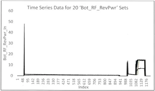
Representative centroids built from the three models discussed above are shown in Figures 11 through 19 for the case of 20 time series of the parameter 'BotRFRevPwr', with black lines indicating the original datasets and the red dashed lines the centroid.

60 Time Series Data for 20 'BotRFRevPwr' Sets

50 40 r 30 Li. c 20 0 10 ccT 0) It W M C -r- H fl -1 in 0 in 0 It t Cc Mc 00 r14 l-r-4 i r14 " c M c M t Ln in (D I'D cc- c- C c 00 M C 0 H -4 Index

(40)

Time Series Data for 20 'Bot_RFRevPwr' Sets, with DBA Centroid m~ 00 r4 m -o~ mO o3 r- :z - m Lfl cj m to m o r- t -' M~ M~ Mt M3 03 r-4 r- N C') N H 4 LY) 0) UL 0) II M~ Zt 1-i rJ C') M3 M3 t U-) Ln k0 (. N- 03 W 0 M MM Index

Figure 12. Time Series and Centroid for Parameter 'BotRFRevPwr', with 20 and DBA Centroid Building Method

Sample Size of

Time Series Data for 20 'Bot_RFRevPwr' Sets, with soft-DTW and Y of 0.001 X3 un "N M t.0M 03 r1 Nc rH -40 ULC) C~j M .0 0 C) zl 03 Zt 03 03 M N C14 N '.LOr n0 L 0) C -4 '- C') 03 03I- -Z Un .ln '.0 . r- r- 03 03 Index -zj' 03 LC) r14 M~ ' a) 03 c 00 CIA N 3 M M 0~ C)C - -4 -4 -41-4 -4

Figure 13. Ti me Series and Centroid for Parameter 'BotRFRevPwr', wi 20 and soft-DTW Centroid Building Method with y of 0.001

th Sample Size of 60 50 C --40 a 30 LL o 20 10 0 00 Lfl C'i) O D W3 M3 03 r14 a~C) C) -4 r-i -- 4 -4r-60 50 40 "30 '0 0 co 10 0 I --

AR

(41)

60 50 J40 CL 30 U-20 10

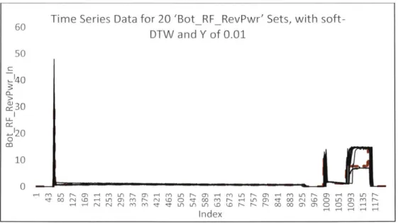
0-Time Series Data for 20 'Bot_RFRevPwr' Sets, with

soft-DTW and Y of 0.01

m On rm-- m y") rN m~ r- m Un r- m~ r- m Ln r- m -1m Lfl

zf w0 r4 CD -i Lfl m~ m0 r- rN 1,o q) - i wo m0 r- r 0q 00 m I

-q -i IN I rj 00 m m i: n in Lr n I Qo r, r- r 0 00 66

Index

Figure 14. Time Series and Centroid for Parameter 'BotRFRevPwr', with 20 and soft-DTW Centroid Building Method with y of 0.01

Time Series Data for 20 'Bot_RFRevPwr' Sets, with soft-DTW and Y of 0.1 00- n U'N M~ r--1 M0 n N- M~ H M0 n N" M~ -1 M0 i) Nl M~ 1 M 17t 00 INj In H uL M~ 00 N- Ij In C) ' W0 00 N --I i) M~ lz W -Ir1Nl ~ IN j MN 00 00 -t Lfl in in I0 Wn N- N- N- W W Index Sample Size of

Figure 15. Time Series and Centroid for Parameter 'Bot_RF_RevPwr', with Sample Size of 20 and soft-DTW Centroid Building Method with y of 0.1

M~ -i 0) inN Ln c) in m- 00n M~ CD C) C) i-1 60 50 140 30 20 10 0 Lfl N m -i m0 in N IN In c) in m~ m0 N M~a CD C) 0 -1

AR

(42)

Time Series Data for 20 'Bot_RFRevPwr' Sets, with soft-DTW and Y of 1.0 -,] rnJ 00 t L t-0 r- 0) M~ C) '- c'j M0 'Z Ln 1.0 r-~ W) M~ 0 ~- " ZT 00 ) (D C) ltr W) (N r- -- Lfl M) M r- 1H Lfl M~ M0 X) (i t -i- ~ r1 (N j MN ( e) 0 T 0 I t Lfn Lfl Q0 kD k-0 f 00 0)W 00 'Zi fln 11 r- W) M CD o I W0 (N 1.0 CD Ir M) M~ M~ MC 0 C) - - -4 r- -q r-4 q -Index

Figure 16. Time Series and Centroid for Parameter 'BotRFRevPwr', with 20 and soft-DTW Centroid Building Method with y of 1.0

Sample Size of

Arithmetic 10%-Winsorized Mean Method

Time Series Data for 20 'Bot_RFRevPwr' Sets, with 60 50 140 S30 0 20 10 0 'Z? W) rN O ) 1:t 0 (W tD C,4 0)--PW ( D C) t 0) (N (.0 C) * 0) CN t.0 -I (N (N r (N 00J 00 rn Tt -t Lfl U-) 1,0 10 0, r-, r-- W) W) W M M Index o 'vt 00 r(N I-0 0 C) 0 0 1H : (N

Figure 17. Time Series and Centroid for Parameter 'Bot_RF_RevPwr', with Sample Size of 20 and Arithmetic Winsorization Method

60 50 140 ' 30 4-1 20 10 0

j

(43)

Time Series Data for 20 'BotRFRevPwr' Sets, with

Arithmetic Untrimmed Mean Method

Lfl (D r- W0 M 0 -H eNj M -c Ll (Dl r. 00 M 0 N. rH if M~ M 00 ej (0 0 17 W0 eNi L 0 IZI M~

Lfl O O .O r- - W0 00 M~ M a) C 0 -1~

index

Figure 18. Time Series and Centroid for Parameter 'BotRFRevPwr', with 20 and Arithmetic Untrimmed Mean Method

Sample Size of

Time Series Data for 20 'BotRFRevPwr' Sets, with

Arithmetic Median Method

,--IN r4 M zr N , - 00 M~ 0 H N- M 1:t Lfl fl N- 00 M 0 r-- " Wc 00 j N 0 -t 00 -H Lr M~ Mf r- r- Lfl M~ MY 00 N fL -1 V- N~ " " flZ) zz l~ Ln u', D t-0 I'D r- - 00 00 M0 -: Lfl .0 N 00 0) 0) W C1 00N Z 0 'Zi M~ M~O~a 0 0 r--1 r. -1 Index

Figure 19. Time Series and Centroid for Parameter 'BotRFRevPwr', with Sample Size of 20 and Arithmetic Median Method

60 50 ~h40 a 30 1 20 10 0 ,-H fj ro -Cz Ln ul . r - W0 M 0 -q (N M 171 ,zj w r-4 Zo o - 00 rj r- --i Lflm ,-- -i r-j r-4 r- t z N 60 50 - 40 a-= 30 U-20 10

(44)

The performance for each method is summarized in Tables 1 and 2 for each parameter. The mean DTW distance is the average DTW distance between the centroid and the time series it is built upon, indicating the quantitative similarity in terms of the distance. The mean SBD is the average SBD between the centroid and the time series it is built upon, indicating the shape similarity. Calculation time is the average time each method spends on each sample size. Both absolute and relative values are listed, with relative percentage value compared to the value for the case where sample size is 20 and the centroid building method is the DBA. Detailed results are listed in Table A. 1 and A.2 in the Appendix.

Table 1. Average Performance of Centroid Methods for the Parameter 'ProChmEndPtChanC' Method 20 Absolute Relative(%) so Absolute Relative(%) 20 Absolute Relative(%) 50 Absolute Relative(%) 20 Absolute Relative(%) Absolute Relative(%)

Soft-dtw Soft-dtw Soft-dtw Soft-dtw Arithmetic Arithmetic DBA (y=0.001) (y=0.01) (y=0.1) (y=1) (Win. Mean) Men)

35475.53' 100.00 45444.34 128.10, 7.501E-037 100.00 1.292E-02' 172.25 7 r 2.60' 100.00 6.25' 240.28 63388.19' 178.68 69314.53 195.39 7.632E-03' 101.75 7.099E-03 94.63. 16.52' 634.90 39.21' 1507.07 51485.33' 145.13 60151.36' 169.56 7.804E-03' 104.04 9.642E-03 128.55 17.01' 653.57 41.20' 1583.40" Mean DTW Distance 46610.46 89177.18 131.39 251.38 64401.14 60729.21' 181.54 171.19 Mean SBD 6.564E-03 7.182E-03 87.51 95.75. 8.091E-031 1.123E-02: 107.86 149.68 Calcualtion Time(s) 17.92 18.05 688.85 693.85 41.671 41.95' 1601.46 1612.38 75229.10' 212.06 76358.67' 215.24 3.789E-03' 50.51 4.240E-03: 56.53 74963.80' 211.31 73359.75' 206.79 3.793E-03' 50.57 4.241E-03' 56.54 Arithmetic (Median) 68661.57 193.55 71756.93 202.27 4.252E-03 56.69 4.771E-03 63.61 0.18 6.76 0.19 7.23 Index Size Index Size Index Size