Analyzing and improving image quality in reflective ghost imaging

Analyzing and Improving Image Quality

Ghost Imaging

by

Nicholas D. Hardy

in Reflective

MASSACHUSETTS INSTITUTE S OF TECHNOJL03Y

M

AR 10 2e"

7277AR

Submitted to the Department of Electrical Engineering and Computer

Science

in partial fulfillment of the requirements for the degree of

ARCHINES

Master of Science in Electrical Engineering and Computer Science

at the

MASSACHUSETTS INSTITUTE OF TECHNOLOGY

February 2011

@

Massachusetts Institute of Technology 2011. All rights reserved.

(~h7 ~.

A u th or ...

Department of Electrical Engineering and Computer Science

January 27, 2011

Certified by ...

us

A. )tratton

Jeffrey I'/ Shapiro

Prof. of Elec. Eng.

Thesis Supervisor

Accepted by ... . . ...

Terry P. Orlando

Chairman, Committee on Graduate Students

Analyzing and Improving Image Quality in Reflective Ghost

Imaging

by

Nicholas D. Hardy

Submitted to the Department of Electrical Engineering and Computer Science on January 27, 2011, in partial fulfillment of the

requirements for the degree of

Master of Science in Electrical Engineering and Computer Science

Abstract

Ghost imaging is a transverse imaging technique that relies on the correlation between a pair of light fields, one that has interacted with the object to be imaged and one that has not. Most ghost imaging experiments have been performed in transmission. and virtually all ghost imaging theory has addressed the transmissive case. Yet stand-off sensing applications require that the object be imaged in reflection. We use Gaussian-state analysis to develop expressions for the spatial resolution, image contrast. and signal-to-noise ratio for ghost imaging performed by measuring a fraction of the light that reflects off a rough-surfaced object that creates target returns with fully developed speckle. This is done for a pseu-dothermal source with phase-insensitive classical correlation between the two fields, and for a quantum source with non-classical phase-sensitive correlation between the fields. In the low flux limit this quantui source becomes the biphoton state. WAe compare our results to

the corresponding behavior seen in transmissive ghost imaging, and we develop performance results for the reflective form of computational ghost imaging. We also provide a preliminary stand-off sensing performance comparison between reflective ghost imaging and a conven-tional direct-detection laser radar system. We also consider the resolution degradation on each system when the fields propagate through turbulence. Finally, we investigate ways of increasing the signal-to-noise ratio of reflective ghost imaging through use of multiple bucket detectors. multiple-wavelength sources, and compressive sensing.

Thesis Supervisor: Jeffrey H. Shapiro

Acknowledgments

The completion of this thesis would not have been possible without the intellectual contri-butions. support. and patience of several people, all of whom I would like to thank. First is my advisor. Professor Jeffrey Shapiro, for his patient guidance and luminous instruction throughout my studies, and careful editing of this thesis. Next is Dr. Franco Wong. for his tutelage in my first few months at MIT, the experience I gained in his lab. and for insightful conversations since. This thesis heavily leveraged framework and theory developed by Dr. Baris Erkmen, whom I would like to thank for his efforts.

I would like to thank my parents. David and Catherine Hardy, for their support.

encour-agement. and always providing a place to call home. I also would like to thank Beverly Chu for her tireless support, editing of this thesis, and for always being my touchstone. Lastly, I would like to thank my fellow members of the Optical and Quantum Communications Group for our shared struggles and triumphs over this last year, and my friends and family for much needed respites.

This work was supported by the U.S. Army MURI Grant No. W911NF-05-0197, and the W. M. Keck Foundation Center for Extreme Quantum Information Theory.

Contents

1 Introduction

2 Ghost Imaging with Pseudothermal Light

2.1

Theoretical Setup . . . ...

2.2

Spatial Resolution and Image Contrast

2.3

Signal-to-Noise Ratio . . . ...

3 Ghost Imaging with Non-Classical Light

3.1

Theoretical Setup . . . ...

3.2 Resolution and Contrast...

..

.

3.3

Signal-to-Noise Ratio.... . . .

. ..

4 Computational Reflective Ghost Imaging

4.1

Theoretical Setup... . . . . . ...

4.2

Comparison to Pseudothermal Ghost hinager

5 Comparison to a Laser Radar System

5.1

Theoretical Setup...

.

. . . ..

5.2

Spatial Resolution and Image Contrast...

. . .

. . . . ...

5.3

Signal-to-Noise Ratio...

. . . .

. .

.

6 Evaluation of Turbulence Effects

6.1

Turbulence Review...

. . . ..

13

13

17

21

27

27

31

33

37

37

39

43

43

45

46

49

49

. . . . . .... . . . . . . . . . . . . . .... . . . . . . . . . . . . . .... . . . . . . . . . . . ... . . . . . . . . . . . . . .... . . . . . . . ... . . . . . . . .. . .. . . . . . . . . . . ... . . . . . . . .

6.2 C lassical Source . . . .

52

6.2.1

Resolution analysis...

. . . .

. . . .

. . . . .

52

6.2.2

Special cases . . . .

55

6.3 Non-classical Source...

. . . .

. . . ..

56

6.4 Laser Radar . . . ...

.. ...

. . ... ..

.

. . . .. . .. . ..

58

7 Improving Ghost Image Quality

61

7.1

Multiple Bucket Detectors... . . . .

. .

. . . ..

62

7.2

Multiple Wavelengths...

.

. . . ..

66

7.3

Compressive Sensing...

. . .

. ..

70

8 Conclusion and Future Work

75

A Detailed SNR Derivation

79

A.1 Pseudothermal Ghost Imager...

. . . .

. . . . .

.

79

A.1.1 Source fluctuations noise term. Ti . . . .

81

A.1.2

Remaining noise ternis...

. . . . .

. . .

. . . .

85

A .2 SPD C Ghost Iniager . . . .

87

Chapter 1

Introduction

In this thesis we explore the viability of using ghost imaging for stand-off sensing. To this end we characterize the image quality of such systems. and compare the results to the image quality of an equivalent laser radar system. We connect our work back to previous theory developed for transmissive ghost imaging, as well as to experiments done in reflection. Finally, we explore ways to improve the quality of reflective ghost imaging. The most promising of these approaches is the application of compressive sensing. which leverages the structure of natural images to reduce image capture time while improving image quality.

Ghost imaging exploits the correlation between two light fields to create an image that neither field alone could provide. We denote these two fields the "signal" and "reference": the signal field interacts with the target, after which a single-pixel "bucket" detector makes a power measurement of the field; simultaneously, the reference field's transverse power dis-tribution is measured with a high spatial-resolution detector. which is usually a scanning pinhole or a CCD array. The signal and reference fields have some cross correlation, de-termined by the choice of source, so measuring the reference field provides some knowledge of the field illuminating the target. Since the power measurement on the signal arm is a function of the target and the field illuminating it. we are able to reconstruct the target by correlating the power measurement with the output of the high spatial-resolution detector. This imaging technique has become known as ghost imaging because the image information

is contained in the correlation between the two measurements: neither measurement alone contains sufficient information to reconstruct the target.

The first ghost imaging experiment used biphoton pairs for the signal and reference fields, which were generated by spontaneous parametric downconversion (SPDC) and post-selection [1]. Because biphotons are entangled states-with a phase-sensitive cross correlation between the signal and reference fields stronger than allowed by classical physics-for which the quantum theory of photodetection is needed to calculate the measurement statistics. it was initially thought that ghost imaging was a non-local quantum phenomenon. However. the non-classical nature of ghost imaging was called into question when experiments were later performed using a classical pseudothermal light source

[2,

3]. In this setup laser light is passed through a ground-glass diffuser, after which it is divided by a 50 50 beam splitter into identical signal and reference fields with a phase-insensitive cross correlation.

Gaussian-state analysis has enabled a unified treatment of biphoton and pseudothermal ghost imaging that shows the image formation process is one of classical coherence propaga-tion, with high contrast in Dc-coupled biphoton ghost images being the principal ghost-image signature of that non-classical source

[4].

In particular, identical statistics for pseudothernal ghost imaging result from the use of quantum photodetection theory, in which both the light beams and photodetcctors are treated quantum-mechanically; and semiclassical photodctcc-tion theory. in which the light beams are treated classically but photodetectors inject shot noise on top of any fluctuations in the illumination. A thorough review of these considera-tions can be found in [5]. For our purposes. it suffices to note that we can-and will-use semiclassical photodetection theory when dealing with classical sources.

To date, Gaussian-state analysis of transmissive pseudothermal ghost imaging has pro-vided expressions for its spatial resolution, image contrast and signal-to-noise ratio (SNR) behaviors; i.e.. a complete characterization of its performance [4, 6]. However, one of the more interesting potential applications of ghost imaging is stand-off sensing, in which the bucket detector observes the target in reflection. not transmission. Preliminary table-top ex-periments have demonstrated the feasibility of this approach

[7,

8], but there has been little

exploration of the statistical characteristics of these images. Developing that theory within the Gaussian-state framework, which is a focus of this thesis, must confront an additional complication not seen in previous work: viz., the speckle induced by reflection from rough-surfaced objects. In particular, we shall report expressions for the spatial resolution, image contrast. and SNR of reflective ghost imaging of speckle targets for classical and non-classical sources in Chapters 2 and 3, respectively. These will be compared with the corresponding results for the transmissive case. in which there is no target-induced speckle. In Chapter 4 we will use this framework to obtain performance results for the reflective form of computa-tional ghost imaging [9, 10], in which the reference beam is removed. Then. in Chapter 5. we will provide a preliminary stand-off sensing performance comparison between reflective ghost imaging and a conventional direct-detection laser radar.

The effects of turbulence on transmissive ghost imaging have been explored experimen-tally [8] and theoretically [11]. As most practical applications of reflective ghost inaging will require propagation through atmospheric turbulence, in Chapter 6 we extend our analysis to include turbulence on all paths. The effects of turbulence on image resolution will be explored for classical, non-classical, and computational reflective ghost imaging, as well as for a laser radar system. In Chapter 7 we explore ways to improve the image quality of reflective ghost imaging. The first of these methods is to employ multiple co-planar bucket detectors on the signal arm; since the target-induced speckle decorrelates with transverse separation in the detector plane, each bucket detector observes different speckle behavior. allowing us to average out its deleterious effects on the SNR. The second method is to use multiple sources at different wavelengths. This again seeks to average out the target-speckle effects: if the wavelengths are far enough apart, the returns associated with each source have uncorrelated speckle statistics. Finally, we extend the compressive sensing methods used in transmissive imaging [12] to reflective imaging. Compressive sensing allows for reduced im-age capture time and higher quality reconstructions when the target is sparsely represented in some basis [13, 14]. Chapter 8 concludes the thesis with a brief summary of results and suggestions for further research.

Chapter 2

Ghost Imaging with Pseudothermal

Light

2.1

Theoretical Setup

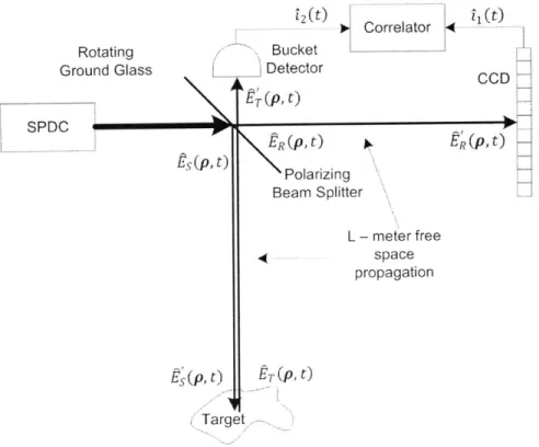
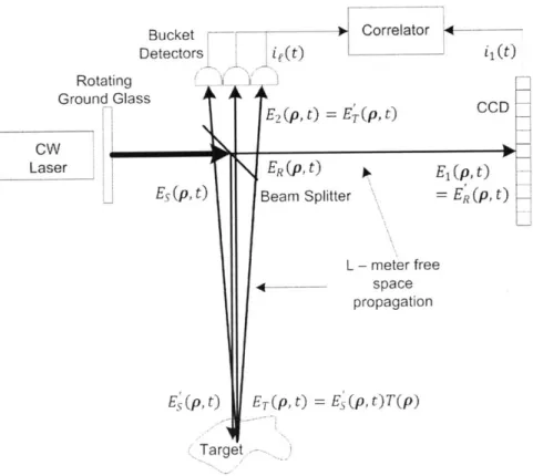
In stand-off sensing, targets will most likely be separated from the source by distances on the order of kilometers. This indicates that high-powered classical sources might be necessary. While we also consider low-flux quantum sources in Chapter 3, we start our analysis with the system shown in Fig. 2-1, which utilizes pseudothermal light to perform reflective ghost imaging. A continuous-wave (cw) laser beam is passed through a rotating ground-glass diffuser followed by a 50 50 beam splitter to produce identical, spatially-incoherent signal and reference beams whose temporal bandwidths are much lower than those of the single-pixel (bucket) and high spatial-resolution (CCD array) detectors. The signal beam illuminates a rough-surfaced planar target at distance L from the beam splitter, and some of the light reflected from that target is collected, after L-m propagation, by the bucket detector. The reference beam directly illuminates the CCD array which, for theoretical convenience. we have placed L-in away from the beam splitter.1 The photocurrents from the bucket detector 'This assumption implies that we will form a 1:1 ghost image. In an actual implementation of reflective

ghost imaging the CCD array would be in the focal plane of a lens located near the transmitter and we would obtain a minified ghost image.

i2 (t)K- (t

--io Correlator -1

Rotating Bucket

Ground Glass Detector

c w

~

2(p~) E~p~t)CCD CW (At) E (p,t)t E t) E (p, =ER E (t Beam Splitter L - meter free space propagation Ei5(pIt) E7(pAt = ES (p, t) T (p) Target

Figure 2-1: Setup for pseudothermal reflective ghost imaging.

and each pixel on the CCD are sent to a correlator, whose output for the CCD pixel located at transverse coordinate pi is

1 pi'/2

C(pi) = dt ii(t)'2 (t), (2.1)

where T, is the averaging time and we have suppressed an L/c time delay in

i

1

(t)

that is

needed to account for the delay incurred by the light returning from the target.

The configuration and notation we are using parallels the semiclassical treatment of transmissive ghost imaging in [9] with the principal distinction being that in the transmissive case the bucket detector would be behind a transmission-mask target L-m from the signal source, whereas here that target is viewed in reflection. We have also switched the labels for the signal and reference fields; in [9] the reference field illuminates the target, while the signal field goes to the high spatial-resolution detector.

linearly-polarized light fields normalized to have V/photons/m 2s units as functions of their transverse coordinate vectors and time. As a result, under the assumption of shot-noise limited detectors with quantum efficiency q. the photocurrents from the bucket and the

CCD can be written as

im(t) Jdr [qPm(r) + A m()] h(t - r), for m = 1. 2. (2.2) Here: Pm(t) =A

fdp

Em(p, t)i2 is the photon flux on the circular active region Am of detector n; q is the electron charge; Aim(t) is the shot noise from detector m; and h(t) is the detector's baseband impulse response, normalized to satisfy fdt h(t) = 1.

Phys-ically, qrPm(t) is the conditional mean of im(t), given the illumination, so that Aim(t)

is the photocurrent fluctuation conditioned on knowledge of the illumination. Note that given the photon-flux waveforms P1(t) and P2(t), the shot-noise currents Aii(t) and Ai2(t) are statistically independent, zero-mean, random processes whose correlation functions are (-Aim(tI)Aim(t 2)) = q

2 _{Pm(ti)(ti - t}

2).

The fields that determine the preceding photon fluxes are found from diffraction theory. applied on three separate patlis: the reference path (R), from the source to the high spatial-resolution detector; the signal path (S). from the source to the target; and the target-return path (T), from the target to the bucket detector. In the ensuing work, we will denote fields that have propagated L-rn on path m with a prime; i.e., if we start with some field Em(p', t),

after L-m propagation it becomes E' (p, t) as

E' (pIt) dp' Em(p'.t) k .eko(L±jpp'12

/2L) m

=

R.

S, T

(2.3)

where ko = wo/c is the wave number. and we have suppressed time delays. The fields are defined as follows: ER(P, t) is the reference field at the source. and EI(p, t) is the field illuminating the CCD: Es(p. t) is the signal field at the source, and E'(p, t) is the field illuminating the target; Er(p, t) = E'(p, t)T(p) is the target-return field. which is

the propagated signal field immediately after reflecting off a target2 _{with field-reflection} coefficient T(p), and E+(p, t) is the field illuminating the bucket detector. Since we are using the semiclassical theory of light, each photodetector is taken to directly measure the classical field impinging it, so E1(p, t) = ER(p, t). and E2(p. t) = El (p. t).

Whereas in transmissive ghost imaging it is ordinarily the case that the target's field-transmission coefficient is assumed to be deterministic, the targets of interest for reflective ghost imaging will have microscopic surface variations-from a nominal, smooth surface profile whose standard deviations can greatly exceed the illumination wavelength and whose transverse correlation scale can be sub-wavelength. When such a surface is illuminated by laser light it gives rise to laser speckle in the target return, and a reasonable statistical model for that behavior is to take the target reflectivity to be

T (,p) = T(p)e2ikoAz(p).

(.

where the height variations Az(p) are modeled as a zero-mean, real-valued, Gaussian random process with a transverse correlation on the order of a wavelength. Thus T(p) is a zero-mean. complex-valued Gaussian random process that is completely characterized by the correlation function [15]

(T*(pi)T(p 2)) = A T(PI)6(p1 - P2), (2.5)

where Ao is the center wavelength of the illumination and

T(p)

is the target's

intensity-reflection coefficient. which is nonrandom and the quantity that we are seeking to image

with the Fig. 2-1 setup.

In order to proceed further, we need to specify the source-field characteristics. Following the Gaussian-state analysis of Erkmnen and Shapiro

[4,

6, 9], we shall assume that Es(p. t) and ER(p, t)-the identical outputs from the 50-50 beam splitter in Fig. 2-1-are zero-mean, coniplex-valued Gaussian random fields that are completely characterized by their common

2

cross-spectrally pure phase-insensitive correlation function per the Gaussian-Schell model as

(EP(pi,

t)Em(P2

.

t2)) = 1 2)/a -p -2 P /2 2-(e2-t 1) 2_/2T

02 C f, m

c

{R,

S}.

(2.6)

lraa

with photon-flux P, e-2 intensity radius ao. coherence length po, and correlation time To.

The preceding setup fully specifies all that is needed to compute the spatial resolution. image contrast. and SNR of the pseudothermal reflective ghost image. Before doing so. however, let us introduce one final condition. We shall assume that the CCD pixel active region.

A

1

,

is sufficiently small that

IE1(p,

t) 12 is essentially constant over each pixel, allowing

us to use

P

1

(t) = AiEi(p,

t)12, where

A

1 is the area of

A1.

This condition ensures that the

spatial resolution we obtain is limited by the field statistics, not by the CCD's pixel size.

2.2

Spatial Resolution and Image Contrast

The spatial resolution and image contrast of the pseudotherinal reflective ghost image are

properties of the ensemble-averaged photocurrent cross correlation, i.e., Eq (2.1) averaged

over the shot noise and the fluctuations in the fields that illuminate the two detectors. Those field fluctuations arise from the randomness imposed by the ground-glass diffuser and, for the

field illuminating the bucket detector, the target's surface roughness. It is easy to see that

the fields illuminating the detectors are zero-mean random processes that are statistically stationary in time, and thus from Eq (2.2) the ensemble-averaged ghost image satisfies

(C(p1)) = (ii(t)i2(t))

Back propagating with Eq (2.3) to the field illuminating the target, the intensity correlation becomes

(IE' (pi.T1)I

2

_{|E'( p', r}

2

)|

2

)k-

L2 Jdp

2

Jdp

3 eika(lp'-31-L'-p2| 2)/2L

x (El*(pi, r1)E'*(p

2

,

T2

)E'

1

(pI.

Ti)E'(p3- T2

)) (T*(p

2

) T(p

3

)),

(2.8)

where we have exploited the statistical independence of E,,

(p.

t) and T(p), i.e.. the fluctua-tions due to propagation through the ground glass and those induced by the target's surface roughness. Equation (2.3) shows that E, (p, t), for m = R. S, is a linear transformation of the zero-mean Gaussian random process E,, (p, t); hence it too is a zero-mean, Gaussian random process. Thus, as in the Gaussian-state analysis of transmissive ghost imaging [4], we employ Gaussian moment-factoring to write the fourth-order field moment in terms of second-order moments. Making use of Eq (2.5) to evaluate the surface moment, and for A2 being the area of

A

2, Eq (2.8) becomes

(ERI(p1, r I12|EIT (p'. 72)12)

=

Jdp

₂

T(p

₂

)

[(|Ej(pi,

i) 2

)(

E'

(p2, 72)| 2)

+

I(E*(pl, T)E'(P2,

2

))|2]

(2.9)

which clearly indicates the role of photon-flux correlation in ghost image formation.

Pseudothermal ghost imaging is performed with spatially incoherent light, i.e., po < ao holds in the source's Gaussian-Schell model spatial correlation. Moreover, stand-off sensing pseudothermal ghost imaging will be performed in the far field, for which koaopo/2L

<

1 prevails. Following Erkmen and Shapiro [5], we can propagate the Gaussian-Schiell correlation function in Eq (2.6) into the far field and obtain

(E'*(P1.

t1)E'

(P2,

t2))

=F 2 C (if+pT/a

Lp

/p

Le-(te22

(2.10)

for

e.

m E

{R. S},

with aL

2L/kopo

and PL = 2L/koao being the new intensity and coherence radii. respectively.

To reduce Eq (2.7) to a form in which we can easily assess the reflective ghost image s spatial resolution and image contrast, we need to define detector's impulse response h(t). For now, let us take this to be a DC-coupled Gaussian of bandwidth QB,3 i.e..

h(t)

=

(2.11)

Because we have assumed that the detector bandwidth is sufficient to follow the temporal behavior of the light emerging from the ground glass, we have that QBTO > 1. This lets us simplify the evaluation of the temporal integrals and obtain

(C(pi)) = 2

a

d ₂ T(p2)e2(IP+1±P-)/al 2 [1 + e-Lpi-p2t/pl) (2.12)

L

aI

When the intensity radius aL is nmuch larger than the target's transverse extent, so that the entire target is uniformly illuminated on average, we get our final form for the ensemble-averaged photocurrent cross correlation.

q 2TI2 AIA42 2P 2 12/p

(Cpi

2 2

r

Jdp

2

T(p

2

)[+

e-[I i-P2|/P2

1.

(2.13)

L

waL

Equation (2.13) shows that the ensemble-average photocurrent cross correlation consists of a featureless background term.

Co

q

2

_AA

2 ) 2

JdP2 T(

2

).

(2.14)

plus the image-bearing tern,

C((1p)

=

dP2 T(P2)e IP . (2.15)

Resolution The image-bearing term contains the target's intensity-reflection coefficient

T(p2

)

convolved with a Gaussian point-spread function (PSF) that limits the spatial

resolu-3

tion to the target-plane coherence length PL = AoL/7rao. This is the same spatial resolution that was previously found via Gaussian-state analysis for far-field transmissive ghost imaging with a pseudothernial source [4]. Indeed, the only difference between Eq (2.15) and the cor-responding result for the transmissive case is the factor A₂

/L

2 _{that appears in the former.}

In transmissive ghost imaging all the light that passes through the target is collected by the bucket detector. but the quasi-Lambertian nature of the rough-surfaced target combines with the stand-off measurement by the bucket detector to introduce the solid-angle subtense factor A2/L2 < 1

in

Eq (2.15).

Contrast Turning now to the image contrast implied by Eq (2.13). we will employ the

contrast definition from

[4].

viz.

m

inax7z[C(p1)] -

inin

7

z[C(pi)]

(2.16)

Co

with the assumption that the target is entirely contained within a region R centered at the origin in transverse coordinates and having a diameter that is much smaller than aL. For simplicity. we will also assume that PL is small enough to resolve all features in the target's

intensity-reflection coefficient. so that

dp

2 T(p2

)e

P1 2 / 7rpT(p1)

(2.17)

and we will take

maxR[T(p1)]

= 1. min- [T(p1)] = 0. Thus

C ~ rp

2

_/AT,

_(2.18)

where AT -f dp2 T(P2) is the effective area of the target. Thus C ~ 1/number of

on-target resolution cells. This image contrast coincides with what was previously derived for

DC-coupled transmissive ghost imaging in far-field operation in

[4].

2.3

Signal-to-Noise Ratio

The featureless background that we encountered in the preceding section can be eliminated

by means of AC-coupling one or both of the photodetectors in the Fig. 2-1 setup. as has

sometimes been done in pseudothermal ghost-imaging experiments

[16].

SNR analysis for transmissive ghost imaging is simplified substantially by inclusion of such AC-coupled detec-tors

[6].

so we shall take the same route here by assuming that the photodetectors' baseband frequency response include a DC block. Specifically, the detectors' frequency response is now modeled by

H BG = -2n2/nQ2 -292/Q2

HB (Q) =e BQ2/ _

e-

NQ/~

(2.19)

where the DC-notch bandwidth, flyN. is much smaller than both fQB, the detectors' high-frequency cutoff, and 1/TO, the source bandwidth.4 With this AC-coupling we have that the average photocurrent cross correlation is background free, viz.. Eq (2.13) becomes

q

2q2

AIA2

(2P

)2IIP 2p

(C(p1))

=qL

A1

21

dp

2

T(p

2

)e'

2 /PA.

(2.20)

Thus it is appropriate to define the ghost image's SNR at the image point pi via

(N, C(pi))2 (C (p 1))2

(.1

SNR (.1

Var

[C(pi)]

(C2(p1)) - (C(p1))2'

i.e, it is the ratio of the squared strength of the image component of the photocurrent cross

correlation divided by the variance of that cross correlation.

Equation (2.20) provides an expression for the numerator in Eq (2.21) and the second term in its denominator. However, to simplify our results. we shall assume that PL is sufficiently small to resolve all features in

T(p),

reducing Eq (2.20) to

A

1

A

2q2 2 (2P) 2

T()

(2.22)

(CQpi)) = L2

7a

2(1) 2 (222

L TraL

4_{Because we have assumed a narrowband pseudothermal source, QNTo < 1 is a more stringent condition}

QB-This leaves us with the formidable task of evaluating

1 ,e1/2

r'i

/2

(C

2

_(p1))

₌

_dt

du

(ii(t)i

2

(t)iI(u)i

2

(u)).

(2.23)

71 -T1/2 J-T 1/2

which requires us to determine an eighth moment of the fields and a fourth moment of the target's field-reflection coefficient. Fortunately, Gaussian-moment factoring can be applied to both of these moment evaluations, but the Fresnel-propagation kernels that canceled out in finding the average photocurrent cross correlation do not do so here. We can simplify the

analysis by using the dimensionless difference coordinate v = pLko(p'- p")/L, where p' and

p" are coordinates at the bucket detector, and defining

A =

jdpT2 p)

A - J 2 , pL (2.24)

F = dv

e

v12/20(v, 4a). (2.26)

where

O((.

D) is the dimensionless version of the two-circle overlap function for circles of diameter D.

O (0 D ) =

CO

co 1D , < D ,( . 7

0, else

a = VA 2

/-ra',

and T($) =F[T(p)](() is the Fourier transform of the target. F was normalized so that it approaches one for very large receiving apertures; i.e., lin,,,, F = 1. Next, we assume that A'r/p2

>

30, which is equivalent to saying that the ghost image

shown in the Appendix, with the resulting SNR being SNR= 2 T FITA+ T2_ -9 T) P["4 _ + ± + + TP1)TOo L2 p2ip

+7

1 1 0 2A2 711 A2 A1 L 3 4,A 2 16v2Aii 2 I2 A₂ (2.28)

where I= PTop 2/a2 is the source brightness in photons per spatiotemporal mode.

Equation (2.28) was written in its full form to allow for any size bucket detector. This is useful when looking at small bucket detectors, such that A2 -> 0; even for high-brightness illumination and a long integration time. we are limited in such situations to SNR < 1 because there is no averaging of the target-induced speckle. However, for a lensed ghost imaging system it is reasonable to assume that the area of the collecting lens in front of the bucket detector is at least as largc as the area of the source beam, or

A

2

/7ra!

;> 1. In this regime, we can simplify Eq (2.28) to

T2(

SNR-2

_T

_P

A'r

+Tp1)To

T

1

7ra6

2A2

+

T(pi) L

2

+

3Air

+ 16xA

1

r

2

L

I

2 v4rp72(p1) LT(p1)ToQBpL

L

2

(2.29)

The terms in the noise denominator of Eq (2.29). which originate from different, comnbina-tions of field variacomnbina-tions and shot noises, have important physical interpretacomnbina-tions. From left to right in that denominator we have: the noise contributed by target-plane speckle from the pseudothermal illumination; the noise contributed by the speckle on the bucket detec-tor arising from the target's surface roughness; the beat noise between the pseudothermal speckle on the CCD pixel and the bucket detector's shot noise; the beat noise between the

CCD pixel's shot noise and the pseudothermal speckle on the bucket detector; and the beat

noise between the shot noises on the two detectors. From here it is of interest to look at the low-brightness (I < 1) and high-brightness (I > 1) SNR asymptotes. These are given by

16&/ Tj

A1ry

2

_I

2

_A

2

SNRL

=

T(pi)

.

(2.30)

and

SNR A- T (2.31)

_AT

7(

-2 T,

F

zraO

2rp2

P1

T 2A2

respectively.

The low-brightness SNR is dominated by the beat noise between the detectors' shot noises. It coincides with the low-brightness SNR found for transmissive ghost imaging

[6],

except for the following two differences: the reflective case has the target's average intensity-reflection coefficient, T(p1), appearing in lieu of transmissive target's

|T(p

1

)|

2; and the reflective case includes the solid-angle scaling factor. A2

/L

2, previously encountered in our comparison of the these ghost imagers' spatial resolutions.

The reflective ghost imager's high-brightness SNR asymptote is controlled by the two speckle terms from Eq (2.29), i.e., the speckle arising from the pseudothermal source's spa-tial incoherence and the speckle arising from the target's surface roughness. Neither speckle noise can be said to universally dominate the high-brightness SNR asymptote. as their rel-ative strengths are governed by both spatial and temporal factors. We need to look at two limiting cases: when the integration time is short enough that the source's spatial incoherence dominates the noise, and when the integration time is long enough that the target-induced speckle dominates the noise. These short integration-time and long integration-time, high-brightness SNR asymptotes are

SNRH.

short-Tj

27-

L

T2

(p

1

),

(2-32)

To A'

and

2 A2

SNRH,

long-Tj -

A2

(2-33)

Here we see the short integration-time. high-brightness SNR for reflective ghost

imag-ing equals the high-brightness SNR for transmissive ghost imagimag-ing with T2(p1) appearing

instead of

|T(p

1

)|

4. This agreement is to be expected, as both of these SNRs are limited

increases, the high-brightness SNR for the reflective case saturates at the value given by

Eq (2.33). Here the SNR is limited by the target-induced speckle. Because we have assunmed

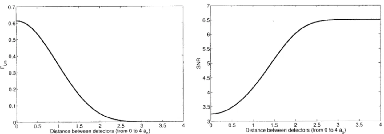
a stationary target whose field-reflection coefficient is constant, no amount of post-detector integration will reduce its speckle noise, and SNR saturation occurs. Furthermore, this effect can be severe: for A2/7ra! = 1 we find SNRH,1OngI' = 3.266, and for

A

2

/7ra2 =

2 we have

SNRH,longT, = 5.54. So, for realistic stand-off sensing, the SNR will be limited to single-digit

Chapter 3

Ghost Imaging with Non-Classical

Light

3.1

Theoretical Setup

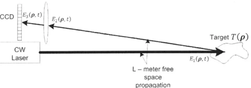
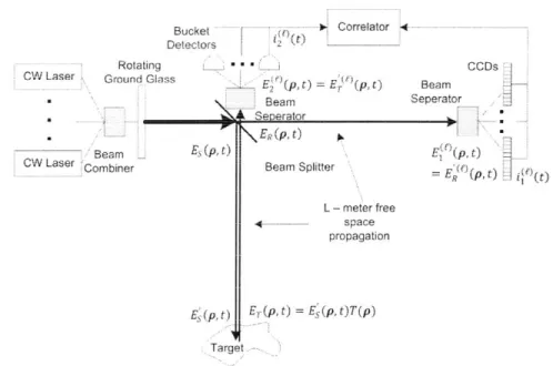
Our analysis of reflective ghost imaging in Chapter 2 focused on a pseudotherial light source with classical phase-insensitive correlation between the signal and reference fields. This setup was chosen because we felt it most closely resembled a system that could be reliably con-structed for experimentation. However, it behooves us to consider alternative light sources. especially those with quantum entanglement between the signal and reference fields. In this chapter we derive the resolution. contrast, and SNR for ghost imagers with phase-sensitive correlation between the signal and reference fields. We work within a Gaussian-state frame-work as done in [4]. exploring correlations ranging from the classical limit up to the quantum limit. But first. we need to reframe our setup in terms of quantum mechanics, as shown in Figs. 3-1(a), 3-1(b), and 3-1(c).

Rotating Ground Glass SPDC es(P

1t)

Correlator Bucket Detector (p, t) !i(t) CCD E (p, t) 'Polarizing Beam Splitter L - meter free space propagation 2s(P, t) $7(p,t)

(a) The output from an SPDC is passed creating signal and reference fields from have a non-classical cross correlation.

through a polarizing beam splitter, the signal and idler photons which

/

R7

(p, t)

(b) For sub-unity quantum efficiency detectors we

have to account for the loss, and inject vacuum to preserve the field commutator relationship. This re-lationship is given in Eq (3.6), and is analogous to the field operator and the vacuum-state operator be-ing passed through a beam splitter of transmissivity

VI]

(c) Since some light is transmitted through the tar-get, the reflected field has suffered loss. We there-fore inject vacuum as in Eq (3.4), which is similar to the field and vacuum passing through a spatially varying beam splitter of transmissivity T(p).

Figure 3-1: The setup in Fig. 2-1 is reframed in terms of quantum mechanics. The source

is changed, the classical fields become field operators, and we have to inject vacuum at the

detectors and target to preserve commutator brackets.

Pi.

(pI

t)

for i

m=T,

ESvacjlm

(p, t)

S(p, t)

T(p) x

=1

x

= 2

J

$vaeC's(p, t)

field operators

Es(p.

t) and ER(p, t). These fields obey the commutator relations

[Ef (pi,

t1),

Em(p

2,

t

2

)]

-0,

(3.1)

[Edpi, t),

E(p

2. t2)] =o,m6(pi - p2)6(ti - t2), (3.2)

where f, m E {S, R. T}. The propagation of the classical fields in Eq (2.3) becomes its operator counterpart

I

koeiko(L+pp'

2|2L)

Em(p~t)

-

dp'Em(p'.t)

i2rL for m - R,

S,T.

(3.3)

The signal and reference field operators have the same basic interpretation as their classical counterparts, i.e., having the statistics of zero-mean Gaussian random processes. but the target-return field description has changed. In order to preserve the field conuntator re-lations in Eqs (3.1) and (3.2), we have to inject vacuum to compensate for the loss at the target. as shown in Fig. 3-1(c) and modeled as

ET(p t) =

E'

(p.t)T(p)

+ vacs(p.t)/l - T(p)|2

.

(3.4)

where Evac.S(p, t) is a vacuum-state field operator.5

The photodetectors can now be thought of as making a measurement of a quantum field operator. Since we are dealing with sub-unity quantum efficiency detectors, we have to inject vacuum-state field operators to maintain the field commutator relationships at the detectors. as shown in Fig. 3-1(b). Thus, our photocurrent is a measurement of the quantum operator

I(t) = q dT dpE.(p.T) Ex(p. T)h(t -- ) for x -1.2, (3.5) J JA A3-5

'Strictly speaking, this expression requires |T(p)1 < 1 for all p. which conflicts with the statistics we have assumed for the field reflection coefficient. However, the A2/L angular subtense factor that we will

encounter on the target return will make our statistics a reasonable approximation for the detected field operator. Also note that the vacuum-state field operator will not contribute to the bucket-detector output.

where

E7(p. t) - VI E (p. t) + y1 - 77 vacm(p, t). (3.6)

and x - 1 for m = R, and x = 2 for m T. For this treatment our source will be an SPDC, whose output is Gaussian-state light with a phase-sensitive cross correlation between

the signal and reference (signal and idler) fields given by [5, 6]

I I

~2P

(p 2

(ER(pit)p, t2)) = 2 4+4)0

The fields will be taken to have no phase-insensitive cross correlation, no phase-sensitive autocorrelation, and a phase-insensitive autocorrelation given by

(E((p1,

t1)E P

(

₂,-t2)) 2 =2e t

2P2

)/a P1-p2/2pge-(tu t1

2_/p2 _m

=R,

S.

(3.8)

Tra5

Looking at the Gaussian-state cross correlation function in Eq

(3.7)

we see two separate correlations. In the low-brightness limit the second term becomes dominant, and the state can be approximated as a biphoton state with a correlation much stronger than the clas-sical limit. Conversely, in the high-brightness limit the first term dominates, and the light approaches a classical state. with the correlation being the same as for the Gaussian-Schell model in Chapter 2. Equation (3.7) captures this full quantum-to-classical behavior, allowing us to say that at low-brightness we have an entangled biphoton state, and at high-brightness we have a classical state with phase-sensitive cross correlation between signal and reference

3.2

Resolution and Contrast

To evaluate the resolution and contrast, we follow the same procedure as for classical light;

i.e.. we look at an ensemble average of the product of the photocurrents as

(C~p1)) = i Z~2(t))

=

q

2

_A1

_dJ1

_{dJT h(t}

-T1

)h(t

- T2)

jdp'

(E4(p1, T) (p'., T2)Z1 (p ,71)$2( p', T2)).

Substituting in Eq (3.6) and recognizing the independence of the zero-mean vacuum fluctu-ations from the field fluctufluctu-ations, we have

(E'(pi, T1)E k(p', T2)Zij(pi. T1)$k2(p', T,2)) = r/2(E" (p1,ITE 715 ( p', 72)5 ( pI T1)$ p',))).

From Eq (3.3) we then find that

(Z( p, ) Ej (p', T2)E'(p1,T1)E(p'.T2)) = Jdp2 dp3 eiko(P P32p 1-p 2 )/2L

x(E

'(p

1. T1)E (P2

-)

2E'

(pi

T1)E' (p3, T2,)))(T* (p2)T(p3)).

once again leaving us needing to evaluate the fourth order field moment after L-meters of propagation., as well as the second order target-surface moment. The target moment is treated in the same manner as it was for classical illumination, and is thus evaluated with

Eq (2.5). Since our fields are normally ordered, and we have Gaussian-state light, we apply

the Gaussian-moment factoring theorem to arrive at

(E'(pi, T1)E(p t )E(pi, T1)El(p', T2))

- dp2 T(p 2) [|59(pi. T1)|

2_)(|$s(P

2, 72)12) + |(E(p1, T1)E'(P2, T2))|12

which is similar to the form we found for pseudothermal light, except that we have a phase-sensitive cross correlation in lieu of a phase-inphase-sensitive cross correlation. To finish the

eval-uation, we need to propagate the phase-sensitive cross correlation and phase-insensitive autocorrelation L meters as follows:

(Ek'(pi, t

1

)E'(p

2

, t

2

))

( 2Pe)

e 2 e1P2j2 e-1I1+P2I/2pL

S 7raf

f

x ± 2 )e(|Pi+/ao 6 (t2-I) 2/2o +

i

2

e( 2+1p2 J2 )/2ag

(t2-t,)2/TJ

(39)

2 7) PTp2

and

(P 7(i ti)E', (P2, t2)) = -2e 2e-( (P2IP12)/alaP1-P2/2pig(t2-ti)/r , (3.10)

7aL

for m = R, S. We can now evaluate the ensemble average of the correlation function, once again assuming that the on-target average illumination pattern is wide enough that it is essentially uniform across the target. With that, we find that the mean of the correlation becomes

q 2rTI2 A1 Au 2P )2 1p

(C(pI))

- j2

<

Jdp

₂

T(p

₂

) I +

e-IP+ 2_/PI

(+

_1j

_(3.11)

where once again I = PTop2/a2. As was done in Chapter 2, this can be broken into the

background term

q

2 72

AIA

2

2P

2

Co

L

2

(

_a

)

_JdP

2

T(0).

(3.12)

L TraL

and the image-bearing term

q

2

r

2

_A

1

A

2

(2P

2 2/P(

C1(P1)

=

2 2

dP2 T(P2)Ikp

/i

2+P2

+.

(3.13)

L TaL _{2 v_2 I}

Resolution Comparing this to our results from pseudothermal illumination, we see that the image is blurred by the same PSF, except that the coordinates are inverted

(p1

-+ -p1). Thus, the image has the same resolution of PL = AoL/7ao.

Contrast Comparing Eq (3.12) to Eq (2.14). we see that sensitive and

phase-insensitive imaging have the same background term. Comparing Eq (3.13) to (2.15), we see that the image-bearing terms differ; this is due to our inclusion of non-classical correla-tions effects. If we look at the high-brightness case. the classical correlation dominates the non-classical correlation, and the image-bearing term for classical phase-sensitive imaging is the same as the image-bearing term for phase-insensitive imaging (except for the coordinate

inversion).

To evaluate at the contrast we will use Eq (2.16), the definition we used for the phase-insensitive imaging. Using the simplifying assumption that the PSF is narrow enough to resolve all target-features, and that

naxz[T(p1)]

1 and min[T(p1)] = 0, we can say

dp

₂ T(p2

)

XIH P2 2

/PL

~ T

-p1).

(3.14)

and simplifv our contrast definition to

AT (2 +i). (3.15)

AT 2v I/_ )-T

where once again AT =

fdp

27(p 2

).

In the high-brightness limit, Eq (3.7) approaches a classical phase-sensitive cross correlation and the contrast in Eq (3.15) approaches Eq (2.18). our result from the pseudothermal ghost imager. However, in the low-brightness limit the the quantum correlation dominates, and the contrast in Eq (3.15) grows without bound. This is the same behavior seen in transmissive biphoton imaging [1. 4]. Thus, maximally correlated phase-sensitive imaging has the same resolution as phase-insensitive imaging, but improved contrast in the low-brightness limit.

3.3

Signal-to-Noise Ratio

The derivation of the SNR for phase-sensitive light will follow what was done in Section 2.3

squared mean to the variance for the image-bearing portion of the photocurrent correlation, which will now be given by Eq (3.13). We will be implementing a DC-block in the detector response as modeled by Eq (2.19), and will assume that the target features are completely resolved by the imager, allowing us to use the simplification in Eq (3.14). With that, the mean of the image-bearing term becomes

C1(p

_C,(P)

1

)

=

q

2

A

1

A

2

q

)

2 7p/T(--p) (2

+ 1).

(3.16)

L2 7ra 2 2-\/27E(

leaving us neceding to evaluate the image-bearing terns second moment

(02(P)) 1 '/2

,/2

(C

2

₍₎₎

₁

T

dt

du

(ii(t)12(t)i1(u)2(u)).

(3.17)

1I ]-T /2 J-T /₂

In evaluating Eq (3.17), we have our first major departure from the derivation in Section 2.3. In Chapter 2 we used a semiclassical treatment of the light, where fluctuations in the measurement were treated as coming from the conversion of the continuous field to discrete charges in the detector, which we called the detector shot noise. However, we are now dealing with quantum-mechanical entangled fields, and must use a full quantum treatment. In quantum optics theory, measurement fluctuations arise from fluctuations of the quantum field. coupled with the type of measurement being performed. Mathematically. these noise terms appear from applying the commutator operations in Eqs (3.1) and (3.2) when normally ordering our higher order field-moments. While the noise qualitatively comes from different sources, quantitatively this has the same effect as the semiclassical treatment: after normally-ordering our fields we have an eighth-order moment, two sixth-order moments. and a fourth-order moment. This comes as no surprise, as it was shown in

[4]

that ghost-image formation using a downconversion source is inherently a classical phenomenon, with the only non-classical features coming from the stronger-than-classical correlation of signal and idler photons. As before, since these higher-order moments are all normally ordered. and the fields are zero-mean, we can apply the Gaussian-moment factoring theorem to express them as the sum of products of second order moments.

We evaluate the moments at a distance of L-meters from the source, using Eq (3.9) for the phase-sensitive cross correlation and Eq (3.10) for the phase-insensitive autocorrelations.

All other second-order moments evaluate to zero. We will again move to the normalized

and difference coordinate v = pLko(p' - p")/L, where p' and p" are coordinates at the bucket detector. The definitions of F, a. AF

and AT

are the same as in Chapter 2. Finally. assuming that there are at least 10 x 10 resolution cells in the image and inverting our coordinate system as pi -- -p1, we have

_Tj. E2

SNR A )

Ar+T/_a__ 0 L2 11p4 a a

2

1p

2vWp T(pl)2 To 2A2T(pi)2 A2IqT(P1) A1Z7 3 4,-A2 16v A2ZE27p

(3.18)

where ]I = + 1). Please see the Appendix for the full derivation. This result is quite

unwieldy, so we would like to simplify it by assuming that the receiving aperture is at least as large as the source aperture., giving us

T(p1)

2

_T

1 2

To

SNR -

_A'

_{TT Dwa% T(p1) L}2

T

_4,wp 2 _{(p1) T(p} 1)/TOQBp2 L2 +(p1)

TT-ta0,2

+ +

~

O'QB+

/2L

p

TO

2A 2

I,

A2 3A 1

Ii

16/5A1I2i}2 A2 (3.19)

This result corresponds to the transmissive result calculated in [6], in the same nIanner as its classical phase-sensitive counterpart in Chapter 2 did: that is. there is now a solid-angle subtense factor on terms associated with the bucket detector. and a target-speckle term in the variance that does not diminish with integration time.

In the classical limit f -± 1. Eq (3.19) becomes Eq (2.29), and we can see that classically correlated phase-sensitive imaging has the same SNR characteristics as phase-insensitive imaging with pseudothermal light. This means that the high-brightness limit is also the same, and is given by Eq (2.31). Now, in the low-brightness limit the quantum correlation

is significant, I[ -+ 21 , and the low-brightness SNR becomes

TI

8A

1

ry

2

I

(320

SNRL =

2T(i) "

(3.20)

T07,QBTO0 2 L 9

This equals the classical low-brightness limit divided by a factor of 2v 2rX, which means

that for I < 1, the low-brightness SNR is orders of magnitude larger for quantum-correlated

light than for classically correlated light. This is the second signature of biphoton state ghost

Chapter 4

Computational Reflective Ghost

Imaging

4.1

Theoretical Setup

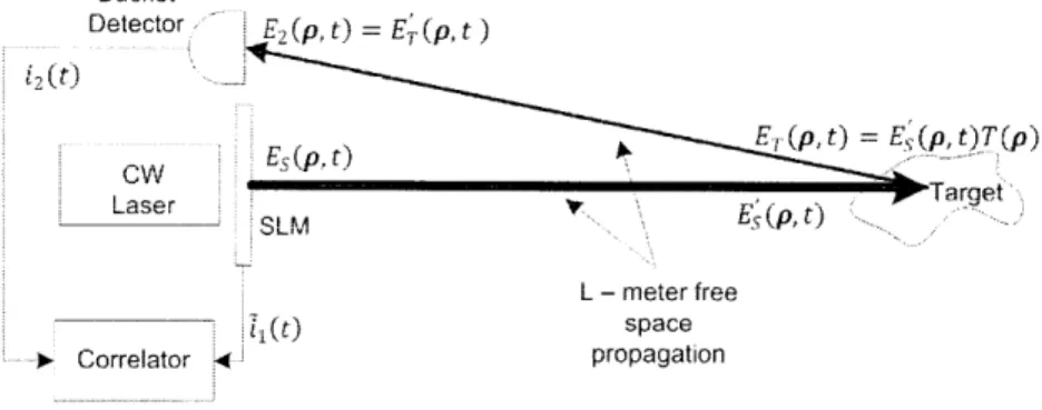
Ghost imaging requires knowledge of the time-varying speckle pattern illuminating the tar-get. Because the ground-glass diffuser in Fig. 2-1 randomly modulates the source field, we measure the reference field's speckle pattern with the CCD array, and exploit its correlation with the speckle pattern impinging on the target to form the ghost image. Suppose, however, that a known source is subjected to a deterministic spatiotemporal modulation, through use of a spatial light modulator (SLM). in a manner that projects a time-varying but determin-istic speckle pattern on the target. In this case the speckle pattern at the target can be computed from diffraction theory, and we do not need the reference arm to form a ghost image

[9].

As shown in Fig. 4-1, we form a computational ghost image by cross correlating the computed reference-arm photocurrent.

Bucket Detector E(p,t)=E(p~t) ptt GW~(p Ept)E ₅ t) E(p, t) T(p)E Laser _SM SLM SCorrelator : Es(p, t) L - meter free space propagation

Figure 4-1: Setup for computational reflective ghost imaging.

with the measured photocurrent, i2(t), from the bucket detector. Here.

PI(t)

=

A1jE(pi, t)|

2

,

(4.2)

gives the computed photon flux for a CCD pixel located at p1 in terms of the computed speckle pattern E1 (pi, t)12.

The SLM is traditionally a square of size D x D, coiposed of a grid of square pixels of size d x d. Each pixel centered at transverse location pt causes a phase shift <p(t) on the light impinging it, imparting a spatially-varying phase shift on the resulting field. This means that. assuming the light hitting the SLM can be approximated as a plane-wave, the field leaving the SLM is

rect

- Y)

e

_(4.3)

where rect(-) is the unit-length rectangle function. p = (x. y), and pt = (x/, y) is the center

of pixel f. Propagating this into the far field results in

E'(p',t) sine I

AoL

(AoL)

s nc

)e-iko(x'xt.+y'y)/L

-iko(|x'\

2_+Iy'2

)/2L i4p(t)

Siic(oL)

where sinc(-) is the sine function, and p'= (x', y').

(4.4)

I arget

4.2

Comparison to Pseudothermal Ghost Imager

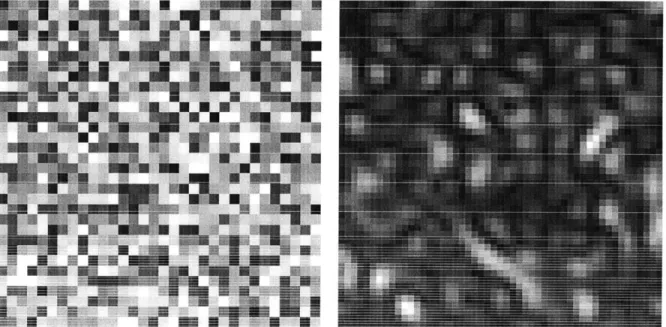
For comparison with the pseudothermal ghost imager, we would like to derive the spatial resolution, image contrast, and SNR of this computational counterpart. Looking at Eq (4.4), it is not immediately clear how to make the connection to imaging with Gaussian-state light. However, as the field in Eq (4.4) is the sum of a sufficiently large number of weighted independent, identically distributed (IID) random variables, from the Central Limit Theorem it will have Gaussian random process statistics [9]. This can be seen in Fig. 4-2, which shows a pseudorandom phase modulation pattern in (a). and the resulting far-field intensity pattern in (b). Thus, we can treat the far-field pattern E

(p.

t) hitting the target and the reference field Ei(pi, t) = E'(p. t) - now calculated from the phase shifts

by Eq (4.4) - as zero-mean. complex-valued Gaussian random processes. Furthermore, to simplify our analysis, we shall assume that we can use the Gaussian-Schell model for the field correlations as given in Eq (2.10). Under these conditions, the far-field coherence length can be approximated as PL = 2L/kOD, and the far-field intensity radius by aL ~ 2L/kd. With these assumptions, all the derivations from Chapter 2 carry over to computational ghost imaging by simple omission of the CCD array's shot noise.

Resolution Under the Gaussian-Schell assumption the spatial resolution of the conputa-tional ghost imager is identical to that of the pseudothermal ghost imager at PL = 2L/kod; therefore, in practice., the resolutions should be similar.

Contrast The computational imager has the same image contrast as pseudothermal ghost

imaging for DC-coupled operation, found in Eq (2.18). Moreover. AC-coupling of the bucket detector's photocurrent or the CCD arrays computed photocurrent will eliminate the fea-tureless background term in the photocurrent cross correlation, giving the computational ghost imager the same high-contrast behavior seen earlier for AC-coupling in pseudotherial