HAL Id: halshs-00586254
https://halshs.archives-ouvertes.fr/halshs-00586254
Preprint submitted on 15 Apr 2011HAL is a multi-disciplinary open access archive for the deposit and dissemination of sci-entific research documents, whether they are pub-lished or not. The documents may come from teaching and research institutions in France or abroad, or from public or private research centers.
L’archive ouverte pluridisciplinaire HAL, est destinée au dépôt et à la diffusion de documents scientifiques de niveau recherche, publiés ou non, émanant des établissements d’enseignement et de recherche français ou étrangers, des laboratoires publics ou privés.
Economic satisfaction and income rank in small
neighbourhoods
Andrew E. Clark, Nicolai Kristensen, Niels Westergård-Nielsen
To cite this version:
Andrew E. Clark, Nicolai Kristensen, Niels Westergård-Nielsen. Economic satisfaction and income rank in small neighbourhoods. 2008. �halshs-00586254�
WORKING PAPER N° 2008 - 44
Economic satisfaction and income rank
in small neighbourhoods
Andrew E. Clark
Nicolai Kristensen
Niels Westergård-Nielsen
JEL Codes: C23, C25, D84, J28, J31, J33
Keywords: satisfaction, neighbours, income
comparisons, geo-coded data
Economic Satisfaction and Income Rank
in Small Neighbourhoods
Andrew E. Clark*, Nicolai Kristensen**and Niels Westergård-Nielsen***
September 2008 Abstract
We contribute to the literature on well-being and comparisons by appealing to new Danish data dividing the country up into around 9000 small neighbourhoods. Administrative data provides us with the income of every person in each of these neighbourhoods. This income information is matched to demographic and economic satisfaction variables from eight years of Danish ECHP data. Panel regression analysis shows that, conditional on own household income, respondents report higher satisfaction levels when their neighbours are richer. However, the individuals are rank-sensitive: conditional on own income and neighbourhood median income, individuals are more satisfied as their percentile neighbourhood ranking improves. A ten percentage point rise in rank (i.e. from 40th to 20th position in a 200-household cell) is worth 0.11 on a one to six scale, which is a large marginal effect in satisfaction terms.
Keywords: Satisfaction, Neighbours, Income Comparisons, Geo-coded Data.
JEL codes: C23, C25, D84, J28, J31, J33.
* Corresponding Author. [email protected]. Paris School of Economics, IZA, and
CCP, Aarhus School of Business, University of Aarhus; ** Danish Institute of Government
Research and CCP, Aarhus School of Business, University of Aarhus; *** CCP, Aarhus
School of Business, University of Aarhus, and IZA. We thank the Rockwool Research Unit, Anna Piil Damm and Marie Louise Schultz-Nielsen for letting us use their work on the geo-coded data, and Anna Piil Damm, Andrew Oswald, Dan Wilson and seminar participants at the EEA conference (Milan) for very useful comments.
1 Getting to Know Your Neighbours
The empirical estimation of social interactions in Economics, which includes the recent work on relative utility, has one essential requirement: identifying those with whom you interact, or who are in the reference group. The broad idea is that individuals compare to, or interact with, others who are in some sense close to them. These can be individuals with whom they identify (salience) or those that they see very often.1
While many different kinds of salient reference groups can be justified ex
ante, it is nigh on impossible to actually prove that any retained reference group
defined by observable individual characteristics (such as age, sex and education) is the “right” one. A frequency of interaction criterion, which will include family, friends, work colleagues, and neighbours, is perhaps easier to defend. It is to this second type of physical closeness, and in particular to neighbours, that we appeal in this paper, to tease out the relationship between individual well-being and others’ income.
A number of existing papers have carried out just such an exercise. Luttmer (2005) showed that individual life satisfaction was positively correlated with own income, but negatively correlated with average income by local area in a number of waves of the US National Survey of Families and Households. Similar findings on American, Canadian, Latin American, and South African data are reported by Blanchflower and Oswald (2004), Graham and Felton (2006), Helliwell and Huang (2005) and Kingdon and Knight (2007), respectively.
Even so, while the motivation for comparing to those who are physically close may seem unimpeachable, there does remain the difficulty of measurement. How can we calculate average income (or some other moment) at a finely-disaggregated level? Survey data is at a disadvantage here. While surveys do provide information on individual well-being, there are rarely enough respondents to provide anything like accurate information at the very local level, producing substantial measurement error, or even empty cells.
Most external datasets also suffer from the same drawbacks as the original survey, leading to relatively aggregated “local” areas that may be thought to stretch the definition of neighbours a little too far. The solution we take here is to match in external data, using population-based information on local neighbourhood
1
Alternatively, the reference group can be directly controlled in an experiment, as in Clark et al. (2008b) and McBride (2007).
characteristics. Particular attention is paid to the homogeneity of the households within these small neighbourhoods, as described below.
2 Matched Geo-coded Data
This paper is based on data of unusual richness. Eight waves of survey data from the Danish sample of the European Community Household Panel (ECHP)2 have been merged with administrative records. The ECHP survey data, which constitute a panel spanning 1994-2001, cover about 7,000 individuals in the first few years. Due to sample attrition this falls to about 5,000 individuals by 2001.
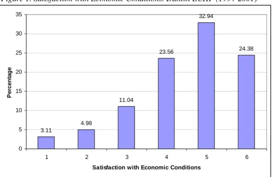
The dependent variable is satisfaction with economic conditions, which is our proxy measure of utility. This is formulated as follows: “How satisfied are you
with your economic conditions? (Please indicate your satisfaction on a scale from 1-6 where 1 signifies “not satisfied at all” and 6 signifies “fully satisfied)”. The
distribution of responses to this question is shown in Figure 1. We assume that the respondent’s answer to this question applies to how well the whole household is doing, not just the individual him/herself. The empirical analysis will therefore relate the respondent’s answer to household income: both her own and those in the neighbourhood.
The Danish component of the ECHP was sampled randomly from the central administrative database, the Central Personal Register (CPR). The CPR contains an entry for each individual in Denmark; each individual has a unique CPR number.
The geo-referenced data comes from a newly-developed data set described in Damm and Schultz-Nielsen (2008). This data set is based on a geographical grid of size 100*100 meters (i.e. 10 000 square meters, or a hectare) covering the entire country. Some of these hectare cells are not inhabited, while others are only very thinly inhabited which poses data confidentiality problems – around two-thirds of inhabited hectare cells contain under five households. Damm and Schultz-Nielsen (2008) have therefore used an aggregation technique to produce clusters of neighbouring hectare cells, where each cluster includes a minimum of 150 households. A second clustering exercise uses the same strategy to produce clusters containing at least 600 households. The priorities in the clustering process were to obtain a classification that does not change over time, is marked out by physical barriers, and is compact, consists of contiguous hectare cells, and is relatively homogenous in terms of type and ownership of housing. In particular, they make sure that the resulting clusters do not contain a major road or waterway, or a
2
See http://epp.eurostat.cec.eu.int for details of the ECHP data.
similar natural boundary. As such, no cluster contains households that are “both sides of the tracks”. Their adjustment process also ensures that an area which consists of mainly single homes is not in the same cluster as an area with blocks of flats (see Damm and Schultz-Nielsen, 2008, for more details).
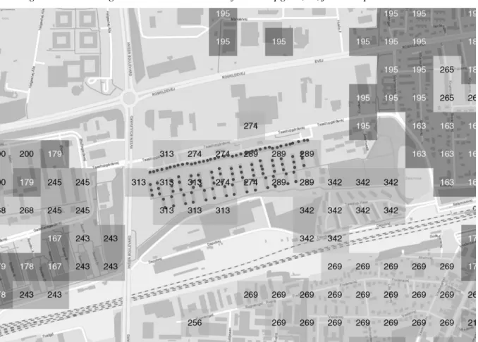
This clustering process transforms the original 431 233 inhabited hectare cells into 9404 and 2296 small and large neighbourhoods respectively (defined by containing a minimum of 150 and 600 households respectively). Figure 2 shows some of the resulting small neighbourhoods in the area of Taastrupgård, Høje Tåstrup (a suburb of Copenhagen). The dots refer to individual addresses which were defined by the government to be “socially-exposed” (in the Government’s Programme Committee for Avoidance of Ghetto areas). The neighbourhoods here match the area well (although the fit is less good in other areas). In general Figure 2 brings out that the constructed neighbourhoods are small: Taastrupgård is divided into three small neighbourhoods of 313, 274 and 289 households in 2004, each containing between 5 and 7 hectare cells (the addresses indicated by the dots in Figure 2 are thus obviously multi-household dwellings).
We then merge the ECHP data with on these small neighbourhoods, matching via the ECHP respondent’s CPR number. Not all small neighbourhoods contain an ECHP respondent, and our regression analysis covers just over 4000 of the 9404 small neighbourhoods mentioned above.
The resulting merged file contains individual-level information, such as demographics (although we will not use the ECHP income information, as discussed below) and our dependent variable, satisfaction with economic conditions. It also contains aggregated information regarding the neighbourhood in which the ECHP respondent lives. This aggregate information on neighbours can take many forms, covering income, earnings, education, and occupation, for example, but also detailed housing characteristics and even behaviours such as new car purchases (again in great detail). The individual-level information refers to all years of the ECHP (1994-2001), while neighbourhood information is available for all years from 1980-2004.
We wish to use this mix of individual- and local-level information to consider the broad question of social interactions. There are a number of ways of looking for evidence of these, as listed below.
• Modelling the behaviour of individual i (ai) as a function of that of her peer group (ai*), where a might represent car ownership, for example:
ai = f(ai*, ….).
• Modelling the utility of individual i (Ui) as a function of both her own and her peer group’s behaviour: Ui = u(ai, ai*, ….).
• Modelling the utility of individual i (Vi) as a function of both her own and her peer group’s income: Vi = v(yi, yi*, ….).
We here consider the last of these, and wish to show that individual well-being is affected by not only own but also peer-group income. Empirical estimation of these kinds of social interactions has been bedeviled by three measurement issues: those of utility, income, and the peer group itself.
For the first of these we appeal to a satisfaction variable, the validity of which has been addressed in Clark et al. (2008a), for example. Second, our key right-hand side variable is income. This is obtained from administrative data for both the ECHP respondent and the local neighbourhood (we therefore do not use ECHP self-reported income), and is arguably fairly free from measurement error because it is double-checked by individuals and employers. We consider household equivalent income (converted using the OECD scale), expressed in real terms in 1980 Danish Kroner. Last, the peer group here consists of the neighbours in the small neighbourhoods, as described above.
The following section shows how own and others’ income are related to economic satisfaction in eight years of panel data.
3 Economic Satisfaction and Neighbourhood Income
We exploit the panel nature of our data to run fixed effect regressions. Table 1 shows some of the results from fixed-effect linear estimation (“within” regressions) of economic satisfaction. The sample consists of around 34,000 observations on 6,800 individuals in 4,000 small neighbourhoods. The two income variables are log of own household annual income, and log of the median household annual income in the neighbourhood (which is less sensitive to outliers than the mean). These both attract positive and significant coefficients in the first column of Table 1. Not only do individuals feel better off as their own income grows, they also feel better off as they live with richer neighbours. Note that these are fixed effect panel regressions, so they are not driven by the inherently satisfied seeking out richer areas. Re-estimating column 1 as a pooled cross-section with clustered standard errors produces a very similar estimated coefficient on neighbourhood income (but a larger estimated coefficient on own household income: “happy” people do indeed earn more).
The regressions in Table 1 also control for a variety of other variables, such as age (which continues to be U-shaped, even within individuals), education, number of years in the neighbourhood, and so on. These mostly attract estimated
coefficients which are consistent with those in the literature. We also control for degree of interaction with neighbours (a dummy variable for talking to them at least twice a week), which attracts a negative but insignificant estimated coefficient.
The results in column 1 may at first sight seem inconsistent with a literature that has insisted on income comparisons in individual well-being. The particular nature of the peer group here may explain why. Having richer neighbours may make me feel worse off in a relative income sense, but have positive spillovers in creating local community social capital. This latter might work through criminality and anti-social behaviour, or via the creation (and funding) of local projects. While it is hard to test directly for many of these, we can address the issue of whether I like having richer neighbours because they pay more taxes and thus provide me with better amenities. Local taxes are not collected at the small neighbourhood level, but rather at the municipality level. To see whether local taxes might explain my preference for rich neighbours, we add, in column 2 of Table 1, a variable showing median municipality household income to the regression. This attracts a completely insignificant coefficient, while that on neighbourhood income remains positive and significant.
An alternative interpretation is that I don’t necessarily want to have rich neighbours per se, but I do like to have neighbours who have the kind of characteristics that attract higher incomes: for example, prime-age, married, and well-educated. The natural test here would be to introduce increasing numbers of neighbourhood demographic variables to see if these are behind the positive neighbourhood income coefficient in Table 1.
We have previously hinted that richer neighbours may induce two counteracting effects: a feeling of lower relative income, but also the possibility of creating local public goods. The final column of Table 1 is a first pass at empirically distinguishing between these two concepts. Here we introduce three income variables: own and neighbourhood income, as in column 1, but also the individual household’s normalized rank in the local income distribution (defined as: rank in neighbourhood / number of households in neighbourhood). Normalised rank is just over zero for the poorest household in the neighbourhood, and one for the richest household. Income rank has previously been appealed to in the context of job satisfaction (Brown et al., 2008) and effort at work (Clark et al., 2008b).
The advantage of normalized rank in this context is that it is unit-free, which helps us to control for the local public goods interpretation. Own household income and median neighbourhood household income only tell us whether the respondent lives in a household which is in the top or bottom half of the local
income distribution. For those above the median, a tighter distribution of local income produces higher rank, whereas for those beneath the median, higher rank comes from a wider distribution.
Rank therefore includes information about the second moment of the income distribution that is perhaps less germane for public-good provision, but is central in determining my own position in the local income ranking. We therefore include it explicitly as a third explanatory variable of economic satisfaction.
The results in column 3 show that, conditional on own and neighbourhood median income, local income rank is strongly positively correlated with economic satisfaction. A rise of ten percentage points in rank is associated with economic satisfaction which is 0.11 higher on the one to six scale: this is a substantial effect. The addition of rank drives the coefficient on own household income down, and that on neighbourhood median income up. This is to be expected. The results in the first column of Table 1 arguably combined several different phenomena. A part of the positive return to own household income is that local rank rises; equally greater median neighbourhood income reduces my own rank, ceteris paribus. Once we control for these rank effects, it is to be expected that own income matters less, and others’ income matters more. The estimated coefficients on all three income variables are significant at the five per cent level.
4 Conclusion
A common theme in the subjective well-being literature has been comparisons to others, but no agreement has been reached on who are these others. One natural definition is in terms of geographical or social distance; the people with whom you rub shoulders every day (friends, colleagues, family, and neighbours). The drawback is that many surveys do not contain sufficient information on these individuals to be useful. Matching from external data sources requires us to identify the respondent’s firm or local neighbourhood. While some work has appealed to such matching, the “neighbourhoods” in question often turn out to be very large indeed.
Danish register data allows us to overcome this drawback, by appealing to many thousands of small neighbourhoods (containing a minimum of 150 households) and administrative data regarding the incomes of everyone in Denmark. We can thus construct truly “local” measures of income, amongst many other things.
We match individual economic satisfaction scores from eight years of ECHP data to measures of both own income and neighbourhood median income,
both derived from administrative data. Our first main finding from panel regressions is that individuals report higher satisfaction levels when their neighbours are richer. Our second finding is that individuals are nonetheless sensitive to their relative position with respect to their neighbours: moving from the 51st percentile to the 100th percentile of the small neighbourhood income distribution is predicted to raise satisfaction by 0.55 points on a one to six scale. While richer neighbours appear to be welcome, being at the top of the pile still counts.
References
Blanchflower, David G. and Oswald, Andrew J. (2004). “Well-being over time in Britain and the USA.” Journal of Public Economics, 88, 1359-1386.
Bolster, Ann, Burgess, Simon, Johnston, Ron, Jones, Kelvyn, Propper, Carol and Saker, Rebecca (2004). “Neighbourhoods, Households and Income Dynamics: A Semi-Parametric Investigation of Neighbourhood Effects.” CEPR Discussion Paper No. 4611.
Brown, Gordon D.A., Gardner, Jonathan, Oswald, Andrew J. and Qian, Jing (2008). “Does Wage Rank Affect Employees' Wellbeing?” Industrial
Relations, 47, 355-389.
Clark, Andrew E., Frijters, Paul and Shields, Michael (2008a). “Relative Income, Happiness and Utility: An Explanation for the Easterlin Paradox and Other Puzzles.” Journal of Economic Literature, 46, 95-144.
Clark, Andrew E., Masclet, David and Villeval, Marie-Claire (2008b). “Effort and Comparison Income.” CEP Discussion Paper No. 0886.
Damm, Anne P. and Schultz-Nielsen, Marie-Louise (2008). “The Construction of Neighbourhoods and its Relevance for the Measurement of Social and Ethnic Segregation: Evidence from Denmark.” Aarhus School of Business, Department of Economics WP 08-17.
Graham, Carol and Felton, Andrew (2006). “Inequality and happiness: Insights from Latin America.” Journal of Economic Inequality, 4, 107-122.
Helliwell, John F. and Huang, Haifang (2005). “How’s the job? Well-being and social capital in the workplace.” NBER Working Paper No. 11759.
Kingdon, Geeta and Knight, John (2007). “Community, comparisons and subjective well-being in a divided society.” Journal of Economic Behaviour &
Organisation, 64, 69-90.
Luttmer, Erzo F.P. (2005). “Neighbors as Negatives: Relative Earnings and Well-Being.” Quarterly Journal of Economics, 120, 963-1002.
McBride, Michael (2007). “Money, Happiness, and Aspirations: An Experimental Study.” University of California-Irvine, Working Paper 060721.
Figure 1. Satisfaction with Economic Conditions. Danish ECHP (1994-2001) 3.11 4.98 11.04 23.56 32.94 24.38 0 5 10 15 20 25 30 35 1 2 3 4 5 6
Satisfaction with Economic Conditions
Pe rc e n ta g e
Figure 2. Small neighbourhoods in the area of Taastrupgård, Høje Tåstrup
Source: Damm and Schultz-Nielsen (2008).
Table 1. Economic Satisfaction, Income and Rank within Small Neighbourhoods: Panel Results
Baseline Baseline and
Municipality
Baseline and Rank
Ln(HH income) 0.390** 0.390** 0.070*
(0.021) (0.021) (0.028)
Ln(median grid HH income) 0.228** 0.236** 0.634**
(0.052) (0.055) (0.057)
Ln(median municipality HH income) --- -0.062 ---
--- (0.156) ---
Relative rank in small grid --- --- 1.124**
--- --- (0.068)
See Neighbours Often -0.019 -0.019 -0.016
(0.016) (0.016) (0.016)
Single -0.057* -0.057* 0.025
(0.027) (0.027) (0.028)
Health problems dummy -0.023 -0.023 -0.023
(0.017) (0.017) (0.017)
Age dummies (9) Yes Yes Yes
Education dummies (6) Yes Yes Yes
Socio-Economic Group dummies (3) Yes Yes Yes
No. and Ages of children dummies (5) Yes Yes Yes
No. Years in Grid dummies (5) Yes Yes Yes
Regional dummies (13) Yes Yes Yes
Year dummies (8) Yes Yes Yes
Observations 33 870 33 870 33 870
Notes: Standard errors in parentheses; + significant at the 10% level; * significant at the 5% level; ** significant at the 1% level. These regressions refer to individuals observed in 4095 small neighbourhoods. These are linear fixed-effect (“within”) regressions.