Demand prediction modeling for utility vegetation management

Demand Prediction Modeling for Utility Vegetation Management

by

Wade Allen McElroy

B.S. Mechanical Engineering, University of Nevada Las Vegas, 2009 M.S. Aerospace Engineering, University of Texas at Austin, 2010

Submitted to the MIT Sloan School of Management and the Department of Mechanical Engineering in Partial Fulfillment of the Requirements for the Degrees

of

Master of Business Administration and

Master of Science in Mechanical Engineering

In conjunction with the Leaders for Global Operations Program at the Massachusetts Institute of Technology

June 2018

K 2018 Wade Allen McElroy. All rights reserved.

The author hereby grants to MIT permission to reproduce and to distribute publicly paper and electronic copies of this thesis document in whole or in part in any medium now known or

hereafter created.

Signature of Author___

Signature redacted

Certified by_

Certified by_

Accepted by_

Accepted by_

Signature redact

MIT Sloan School of Management Department of Mechanical Engineering May 11, 2018

:ed

Georgia Perakis, Thesis Supervisor William F. Pounds Professor of Management MIT Sloan School of Management

Signature redacted

Konstantin Turitsyn, Thesis Supervisor Professor, MIT Scpool of Engineering

Signature redacted

Maura'erson Director, MIT Sloan MBA Program

AT loan School of4anagement

Signature redacted

Rohan Abeyratne Professor and Graduate Officer MIT Mechanical Engineering

/ 1 MASSACHUSETTS INSTITUTE OF TECHNOLOGY

JUN 0

7

2018

LIBRARIES

_

This page left intentionally blank

Demand Prediction Modeling for Utility Vegetation Management

By

Wade Allen McElroy

Submitted to the MIT Sloan School of Management and the MIT

Department of Mechanical Engineering on May 11, 2017 in partial fulfillment of the requirements for the degrees of Master of Business Administration and Master of Science in

Mechanical Engineering

Abstract

This thesis proposes a demand prediction model for utility vegetation management (VM) organizations. The primary uses of the model is to aid in the technology adoption process of Light Detection and Ranging (LiDAR) inspections, and overall system planning efforts.

Utility asset management ensures vegetation clearance of electrical overhead powerlines to meet state and federal regulations, all in an effort to create the safest and most reliable electrical system for their customers. To meet compliance, the utility inspects and then prunes and/or removes trees within their entire service area on an annual basis. In recent years LiDAR technology has become more widely implemented in utilities to quickly and accurately inspect their service territory.

VM programs encounter the dilemma of wanting to pursue LiDAR as a technology to improve their operations, but find it prudent, especially in the high risk and critical regulatory environment, to test the technology. The biggest problem during, and after, the testing is having a baseline of the expected number of tree units worked each year due to the intrinsic variability of tree growth. As such, double inspection and/or long pilot projects are conducted before there is full adoption of the technology.

This thesis will address the prediction of circuit-level tree work forecasting through the development a model using statistical methods. The outcome of this model will be a reduced timeframe for complete adoption of LiDAR technology for utility vegetation programs. Additionally, the modeling effort provides the utility with insight into annual planning improvements. Lastly for later usage, the model will be a baseline for future individual tree growth models that include and leverage LiDAR data to provide a superior level of safety and reliability for utility customers.

Thesis Supervisor: Georgia Perakis

Title: William F. Pounds Professor of Management Science, MIT Sloan School of Management Thesis Supervisor: Konstantin Turitsyn

This page left intentionally blank

Acknowedgments

I would like to thank the team of vegetation management experts that assisted in this work. Your unwavering support and attention to this project was noticeable and meaningful. The task that you all take on is an important one, and I'm glad that you took the time to consider my contributions in making that work a safer, more reliable, and better for all of the residents in the service territory.

I'd like to thank my thesis advisors Georgia Perakis, and Kostya Turitsyn for their support of this work. Additionally, I'd also like to thank the Leaders for Global Operations program for their guidance and support throughout the program.

I'd like to thank my parents Dave and Kim McElroy who have shaped me into the person that I have become today. Without your guidance, support, lessons, humor, and spirt I would have never been able to accomplish anything that I have. And lastly, I would like to thank my girlfriend Nicole who supported me throughout this entire two year adventure. Your kind words, subtle motivation, helpful and lighthearted distractions, endless ability to listen, incredible and unparalleled outlook on the world, and outright excellence in all that you do drove me to be just a bit better. I could not have asked for a better companion to have by my side on this journey.

This page left intentionally blank

Contents

1

Introduction and Background ... 13

1.1 U tility V egetation M anagem ent O verview ... 13

1.2 Technology Adoption in Vegetation Management ... 15

1.2.1 R em ote Sensing ... 15

1.2.2 T ree G row th M odeling ... 16

1.3 P roblem Statem ent and G oals... 16

1.4 Focus of Project... 17

1.4 .1 D istribution ... 17

1.4 .2 Circuit Level... 17

1.4.3 R outine T rim s ... 18

1.5 T hesis H ypothesis ... 18

1.6 T hesis Contributions and O utline... 18

1.7 L terature R eview ... 19

2 D ata Sources... 2 1 2.1 O verview ... 2 1 2.1.1 W ork M anagem ent System (W M S) ... 2 1 2.1.2 Project M anagem ent D atabase (P M D ) ... 22

2.1.3 T ree G row th D ata ... 22

2.1.4 Circuit Location Inform ation ... 22

2.1.5 W eather D ata... 23

2.1.6 D rought D ata ... 23

2.1.7 Practices V ariable ... 24

2.2 Preparing the D ata Set ... 25

2.2.1 W eather D ata... 25

2.2.2 Creating Running Average and Standard Deviation Parameters... 26

2.2.3 Sp ecies G row th D ata ... 27

3.1 D istribution of Trim s ... 29

3.2 W eather D ata ... 32

3.2.1 Tem perature D ata ... 32

3.2.2 Precipitation Inform ation ... 35

3.2.3 D rought Data ... 37

4 M odeling A pproach ... 39

4.1 O verview ... 39

4.2 D ata Fram e and Variable Selections ... 39

4.3 T est and Training Split ... 40

4.4 Clustering M ethods ... 40

4.5 M odels ... 40

4.5.1 Stepw ise Linear Regression ... 4 1 4.5.2 CA RT ... 41 4.S.3 Random Forest ... 42 4.6 A ccuracy M easures ... 43 4.7 Final A pproach ... 44 5 M odel Results ... 45 5.1 Baseline M odels ... 45 5.2 V ariable Selection ... 45

5.2.1 Tem perature V ariable Selection ... 46

5.2.2 Precipitation Variable Selection ... 46

5.2.3 D rought V ariable Selection ... 47

5.2.4 Practices V ariable ... 48

5.2.5 Species and PM D V ariable Selection ... 48

5.3 Clustering M ethod Results ... 49

5.3.1 Clustering M ethods ... 49

5.3.2 Clustering Size Verification ... 49

5.3.3 Inter-M odel Errors ... 51

5.4 Input D ata Treatm ents ... 52

5.4.1 Outlier Refinem ent... 52

5.4.2 Normalization and Final Model ... 53

5.5 Variable Significance ... ... 54

5.5 .1 L n a o e Variables i n fc n e ... 54

5.5.1 Linear M odel Variables ... 55

5.5.2

V ariable

Inflation

Factors...

56

6 Conclusions and

Im

rove m ents... 7

6.1 Recom m endations ... 57

6.2 General Fin dings... 57

6.3 Future W ork...

58

Appendix A: List of Acronym s ... 60

Appendix B: All M odels Accuracy Table ... 61

A ppendix C: All M odel Accuracy Table in Rank Order ... 62

List of Figures

Figure 1: Electrical Compliance Example ... 13

Figure 2: Vegetation Management Program Process Flow Diagram ... 14

Figure 3: Representative LiDAR point cloud... 16

Figure 4: NOAA U.S. Climatological Divisions ... 24

Figure 5: Operational Calendar for System Analyzed ... 25

Figure 6: Weather Station Distance Density Plot for 2017 Circuits ... 26

Figure 7: Divisional Breakdown of Tree Growth Rate Types... 27

Figure 8: Total Trims Probability Density by Year... 29

Figure 9: Log Transformation of Total Trims Probability Density by Year... 30

Figure 10: Transformation of Total Trims by Normalization ... 30

Figure 11: Total Trims Box Plot by Year ... 31

Figure 12: Total Trims Box plot by Year without outliers... 31

Figure 13: Temperature Data Correlation Matrix... 32

Figure 14: Correlation Plot for Winter Temperature Variable... 33

Figure 15: Boxplot of Minimum Average Temperature by Season and Year... 34

Figure 16: Boxplot of Average-Average Temperature by Season and Year ... 34

Figure 17: Boxplot of Days Below 32 degrees F by Season and Year ... 35

Figure 18: Precipitation Data Correlation Plot... 36

Figure 19: Boxplot of Total Precipitation by Season and Year ... 36

Figure 20: Drought Index Correlation Plot ... 37

Figure 21: Boxplot of Modified Palmer Drought Index (PMDI) over Years ... 38

Figure 22: Modeling Approach Flow Chart... 39

Figure 23: K-Mean Clustering Size Accuracy Plots ... 50

Figure 24: Units Clustering Size Accuracy Plots ... 50

Figure 25: Scatter Plot of Model Error by Unit Cluster... 51

Figure 26: Scatter Plot of Model Error by Z-Score for Training and Testing Datasets ... 52

List of Tables

Table 1: Baseline Model Performance ... 45

Table 2: Temperature Variable Selection Model Performance ... 46

Table 3: Precipitation Variable Selection Model Performance... 47

Table 4: Drought Index Selection Model Performance ... 47

Table 5: Practices Variable Model Performance... 48

Table 6: Species and PMD Variable Model Performance ... 48

Table 7: Clustering Method Model Performance... 49

Table 8: Individual Cluster Model Performance... 51

Table 9: Outlier Removal Model Performance ... 53

Table 10: Normalization Model Performance ... 54

Table 11: Linear Model Cluster Standardized Coefficients ... 55

Table 12: Linear Model Variable Inflation Factor (VIF)... 56

List

of Equations

Equation 1: Out-of-sample R2 . . . ... 43

Equation 2: Root Mean Square Error ... 43

Equation 3: Volume Weighted Mean Absolute Percentage Error ... 43

Equation 4: Symmetric Mean Absolute Percentage Error... 43

Equation 5: Naive Model Formulation... 45

This page left intentionally blank

1 Introduction and Background

1.1 Utility Vegetation Management Overview

Utility vegetation management (VM) programs provide preventative maintenance for asset management; for this thesis the focus will be on trees and electrical power conductors. Vegetation surrounding assets are regularly trimmed or removed to prevent growth that would otherwise damage the assets. The work is completed in accordance with both state public utility commission and federal regulatory requirements. Examples of regulatory requirements are depicted in Figure 1, and show that the risk to assets is predominantly focused on physical clearance from the conductor. VM work is critical to a utility safely and reliably providing service in its territory, but can also present large challenges. One notable challenge is that scale associated with ensuring that the entire system is within compliance, where a system network or grid can span over 100,000 miles of overhead conductor and in excess of 100 million trees within reasonable proximity.

Figure 1: Electrical Compliance Example1

In response to the issues of large scale with high regulatory compliance metrics, VM groups will deploy a program similar to the one shown in Figure 2 to provide routine tree work. The major facets of VM programs are:

* Planning and scheduling of work: when covering the entire service territory it is critical to create a plan for the expected workload, it is customary for utility planners, patrollers, and tree workers to participate in this planning session.

* Circuit patrols: consist of visual inspection, typically by walking, of an entire circuit and identifying specific trees that have the potential to become out of compliance in the given year -presumably all of the trees visited will be in compliance and will only need to be worked for growth in the coming year.

" Performing tree work2: where the trees that have been prescribed work from the patrols

are physically treated. The tree crews will apply best practices for preforming the trims as to not harm the long-term health of the tree, but also strive for a trim that will not require revisiting the tree for multiple years3.

* Quality assurance and control: quality steps occur following a patrol and/or a tree

working step to ensure that standard procedures and regulatory requirements are followed. Examples include, verifying that trees that needed to be prescribed were, and conversely trees that did not require work were not.

The two most significant areas of work revolve around patrols and tree work. Patrols are performed for the entire service territory by trained specialists that prescribe work to ensure that both the utility assets are protected and to ensure the trees remain clear of electric facilities. The tree work prescription is then provided to an independent group or company that carries up the defined tree service. Lastly, another level of inspection, quality assurance and control, is conducted on both the patrol and tree work to confirm the general process does not have any issues. Utilities can select to perform this process over any time frame they deem suitable to stay within regulatory compliance; a typical selection is annually.

Routine Operations

Create Curdent Year C efrPesibd

Inspection / Quality

Conducted separate and randomly after work s completed in Routine Operations process

Employee

r

Ire

Key:-

L~JLj

Figure 2: Vegetation Management Program Process Flow Diagram

2 Tree workis a general phrase in vegetation management to imply the trimming and/or removing of trees

to provide adequate clearance.

1.2 Technology Adoption in Vegetation Management

Despite the possibility to implement VM programs with a relatively manual process, new technology has and will continue to play a key role in VM. The linkages in the routine operations of Figure 2 between the utility, patrol, and tree crews in the field have been aided by the implementation of a digital records system over the last 20 years. This digital system has built up to include instantaneous generation of electronic work instructions, tracking work progress, and quick and reliable access to previous work conducted. In recent years, VM programs have been investigating and testing the possibility for the following technologies to improve their operations reliability and efficiency.

1.2.1 Remote Sensing

One major area of assistance for VM programs comes via remote sensing technologies, or electronic observation from a distance. Within this broad definition there exist multiple sensor packages and even further platforms to deploy these sensors. Each of the sensors can span wide ranges of spectra from infrared to ultra violet, and can be installed on platforms that include: unmanned aircraft systems (UASs, or more commonly referred to as drones), rotary aircraft (helicopters), fixed-wing aircraft and orbital satellites. Although all of these potential systems can provide meaningful information to vegetation managers, Light Detection and Ranging (LiDAR) on fixed wing aircraft has provide the greatest promise.

LiDAR is a technology that uses the reflection of visible light to measure distance. The system collects numerous distance measurements (on the order to 2 to 100's of points per square meter) by performing continuous swaths of the system and finally creating what is referred to as a point cloud. Figure 3 shows a representative point cloud that contains millions of induvial points that make up multiple trees, houses, and utility lines. The color of the individual trees in Figure

3 signifies unique tree species, which is determined through the process of hyperspectral4

imagery analysis. This information is then fused with the LiDAR point cloud to produce a multivariate, single data set.

4 _{Hyperspectral refers to additional sensors information that is acquired in the infrared, visible, or}

ultraviolet wavelengths that is then mapped to the individual LiDAR point cloud point. In essence appending additional information to that point in 3D space.

Figure 3: Representative LiDAR point cloud'

The key advantage of LiDAR to vegetation mangers is the ability to quickly and accurately acquire information on the clearance between vegetation and conductors over thousands of miles of overhead electrical lines, while also producing a data source that can be revisited and reused. Under the current system, people are required to manually patrol the entire network to make visual inspections that cannot be re-examined outside of their recommended prescriptions without physically revisiting the site.

1.2.2 Tree Growth Modeling

An additional advantage of LiDAR is extremely granular information about individual trees. Currently VM programs focus at the parcel level and the number of trees located at that parcel. However, the continuity of an individual tree record is not guaranteed. With the implementation of LiDAR, tree level records will be available, if not required. In practice the information gathered could even be one level lower at the individual branch levels, as this is fundamentally what is measured in a LiDAR scan and trimmed by the tree crews. With this added information it would be possible for VM programs to investigate the use of tree growth models. At its fullest capability, this would allow for a process flow where patrolling of a circuit may not be required, as the system would have a statistical prediction of whether each tree needs work or not. A future state system like this would be extremely challenging, if not infeasible, without the measurements provided by LiDAR.

1.3 Problem Statement and Goals

Despite all of the advantages of implementing a LiDAR program, an issues arises with technology adoption, where VM programs encounter the dilemma of wanting to pursue LiDAR as

a technology to improve their operations, but still cannot immediately trust the output data. Subsequently, the VM groups find it prudent, especially in the high risk and critical regulatory environment, to test the technology. The nature of the test would be comparing the number of detections6 to an expected value provided externally or by direct comparison to a human patroller. However, during the testing process, a problem arises associated with how to anticipate the number of detections given the degree of variability in the number of units worked annually. The goal of this thesis is to address the problem of unknown circuit-level tree work counts by applying modern statistical methods to predict annual trees worked, and variables that are influential to those deviations. The result of applying this model will be a decreased timeframe for full scale adoption of LiDAR technology for utility VM programs.

1.4 Focus of Project

Within VM programs there are details, such as groupings of work, which are not fully covered in Figure 2. In order to properly scope the predictive model, focus areas were required to make the model both general enough to be comprehensive, yet detailed enough to provide accuracy and usefulness. The result of this scoping is a model concentrating on the distribution system for routine trims on an annual basis for circuits. Below is further explanation of the decisions made in the scoping effort.

1.4.1 Distribution

The scope will be on the electrical distribution system. Although a model could be created separately for a transmission system, the differences in regulatory structure made it more suitable to only provide a model for distribution circuits.

1.4.2 Circuit Level

The scale of the model will be at the circuit level. Utilities, and VM programs by association, will customarily divide required work within the service territory by a geographic hierarchy from the full system to geographic divisions to circuits. Where circuits are the general name given for a contiguous stretch of conductor from the distribution substation to the termination of the line, the model will attempt to predict at this level. This selection was made due to the applicability to LiDAR detections and furthermore to the general work planning structure used in VM programs. Divisions and systems were not selected, or even analyzed, because data inconstancies and nuances were found at the individual circuit levels. Furthermore, individual trees in a logistic model (trim this year or not) were not pursued because the data was not yet available with any confidence.

6 Detections is a term used to imply a set of criteria, mostly distance, are met for an induvial tree as

determined through LiDAR data analysis. For example, if using Figure 1 for Distribution a LiDAR detection would be when a tree is found to be within 10 inches of a conductor. Although this is inside of the regulatory compliance range, the detection distance and logic can potentially be greater.

Lastly it is critical to distinguish that predictions are made for each circuit on an annual basis which, for ease, will be referred to as a circuit-year. This grouping is reasonable as the patrol and tree work for an individual circuit is traditionally carried out on an annual basis over a couple week span.

1.4.3 Routine Trims

The unit being predicted will be tree trims. This base unit is applied mainly because it is the most commonly performed VM program operation, as well as the clearest to predict. However VM programs conduct other work, a few of additional services that are performed but not included in the prediction model are:

" Brush: not all trees have clear distinct branches that can be trimmed and tracked, instead brush units can be applied to wispy branches that are measured on an approximate volume removed compared to a single tree.

* Removals: at times patrollers may prescribe the removal a tree, for example there are some fast growing species that may have grown to a point where compliance may not be guaranteed and removing the tree is the best course of action. Note, this value is still included in the model because a tree that was worked over many prior years that will not be worked in the future due to removal could be helpful for prediction.

* Hazard Trees: in the case of a dead and dying tree, patrollers will prescribe a unique removal associated with unhealthy trees.

* Proactive Reliability Tree Work: this group of tree working, both trims and removals, is related to additional operations that are conducted in a truly preventative fashion. The trees in this category are healthy and not out of compliance, but are a risk to safely and reliably providing electrical service. This work can be conducted for example on specific species that might be subject to shedding branches, or geographically based on historical weather issues that have resulted in downed power lines.

1.5 Thesis Hypothesis

The hypothesis tested in this thesis is that with statistical modeling it is possible to predict the number of number of trees trimmed in a given circuit-year at a higher accuracy than a naive model or simple running average. The increase in model accuracy is attributable to a collection of additional variables that help indicate the number of trees worked, in addition to clustering similar circuits before to model creation.

1.6 Thesis Contributions and Outline

This thesis describes the process of creation, rationale, and results for numerous predictive models from a representative vegetation management program. In Chapter 2, the assumptions, sources, and variables implemented, and more importantly variables excluded, from the data

frames have are discussed. Chapter 3 conducts data exploration consisting of plotting of the variables presented in Chapter 2 to inform the model creation process, with a specific emphasis on avoid selecting collinear variables. Chapter 4 describes the statistical models implemented, the assumptions made with each of the models input variables, and lastly describes the process to be implemented for variable and model selection. Chapter 5 presents the results of the modeling process and short comings observed from the multiple model combinations that could be implemented. The final result is a model that marginally improves the volume weighted Mean Absolute Percentage Error (vwMAPE), by 1.1%, and symmetric Mean Absolute Percentage Error (sMAPE), by 0.3%, over a simple running average prediction. Although these seem to be less than stellar results form a predictive sense, the results provide guidance for LiDAR adoption, meaningful variables, as well as overall vegetation management operations procedures. Finally Chapter 6 provides summarized findings, recommendations of future work, and major contributions. Below is a list of the notable contributions:

" The most useful predictive variables are the US Drought Monitor Index values and VM program process improvements metrics

* Continuous weather variables, not discrete variables that contain for example the

number of days a criteria is met, are superior for tree trim prediction

" Average weather variables, not extremes for a time period, are superior for tree trim prediction

" Clustering prior to modeling created marginally better performance, with clustering by the running average number of units being superior to other more sophisticated (i.e. K-Means) clustering methods

* Linear regression returns superior models than CART and Random Forest models

1.7 Literature Review

Previous research in the area of vegetation growth predictions have focused in two major areas: large scale growth patterns and local growth of pruned high value vegetation; such as, olive trees [1], and pears [2], where pruning is used as a way of increasing growth and subsequently the per plant yield.

Large Scale Growth Modeling -The large scale growth research has developed multiple growth models, with seminal analytical publications starting around 1933 [3]; however, when applied to separate regions and/or problems numerous modeling updates have been evaluated in [4] [5], and [6]. [6] focused on vegetation management as whole, and presents a four-tiered system of models that consider temporal aspects of modeling from strategic planning (50-100 years), long-term planning (10-15years), multiyear planning (3-5 years), and operation planning (up to 1 year). Similar to the range in years of models, the variables considered also have wide range is the physical size and diversity - from individual tree growth mechanism at the cellular

level, to tree nutrient completion and shading at the forest level. Some attempts have been made in vegetation management groups to predict individual species growth in small samples [7], but the largest research focus has been related to predicting vegetation outages [8], [9], [10].

Local Growth Modeling -More recent studies [1], [2], [9] have begun investigations into local growth via the use LiDAR based data as a variable, with specific research traction in the applications of pruning volume perditions for biomass energy use [1]. Although research into tree growth modeling has been conducted across a wide array of topics and variables, the regime of vegetation growth pertaining to utility trim predictions on an annual level is a limited.

However, the research in the area of predictive modeling at utilities has become more common. For example, prior work from [8], [11], and [12] have shown promising results when applying statistical modeling to utility based questions. Specifically, [8] highlights the value of vegetation-related data.

2 Data Sources

2.1 Overview

There are six main data sources that were used for the creation of the data frame analyzed: Work Management System (WMS), Project Management Database (PMD), Tree Growth Data, Circuit Location Information, Weather Data, and Drought Data. In total these databases combined to create a data frame of 14 project years, comprised of 35,960 circuit-years, and 100+ variables that could be utilized for prediction.

2.1.1 Work Management System (WMS)

The Work Management System (WMS) is the database that contains all of the tree work that has been conducted in the service territory for the last 15+ years. For the purposes of the data frame creation, information was evaluated from 2001 to 2017. The variables provided from this database include:

* Total Trims: the prediction variable for the models; it depicts the number of routine trims

that occurred in a given circuit-year.

* _{Project Year: the organizational year in which tree work is conducted. Assumed to begins}

on October 1 and ends on Sept 30 of the following year. For example, work conducted on circuit ABC between October 1, 2016 and September 30, 2017 is assigned to the 2017 project year.

* _{R1 Removals: are a specific group of removals for trees that have a diameter at breast} height (DBH) of less than 12 inches but greater than or equal to 4 inches. All removals less than 4 inches are considered Brush and not counted in this metric.

" Division7: the regional grouping created by the VM group to divide work evenly. This categorical variable was included but not used in the data frame as a potential clustering variable where historical groupings could have nuanced meanings not fully described by the other variables.

* Species Trim Data: the Total Trims variable is an aggregation of individual tree trim records. For instance, these records will indicate that on 12/23/2007 a Palm Tree with a DBH of 17 inches was trimmed at 123 Main Street on Circuit ABC. Although plenty of information is contained in this type of record, the purpose was to obtain the specific species information and combine all of the identical species records up to the circuit level. The final result being circuit-year ABC-2007 had X Palm Trees, Y Black Oaks, Z Orange Trees, etc. The result of this system is combined with information from Tree Growth Data in Section 2.2.3.

2.1.2 Project Management Database (PMD)

The Project Management Database (PMD) is similar to WMS in that it provides insight into the trims conducted in a circuit-year; however, the PMD contains additional information about the project in that year. Some of the unique project level information found in PMD is:

* Project Quarter: organizationally VM programs might elect to group circuits by seasonal quarters for planning purposed. Similar to the Divisions variable it is included as a way of exploring potential grouping of circuits made by VM experts.

* Planned Units:8 at the beginning of a project VM mangers are required to insert a planned number of trims. Presumably this variable is a culmination of knowledge and negotiation with patrollers and tree trimmers in the field. Although this is included in the data frame, it was excluded from model creation due to a high degree of variability for the actual units. This variability is assumed to be by mangers not applying a consistent timing and rationale for updating this variable.

* Tree Contractor:9 is a categorical variable for the group that provided tree work for that circuit-year, as it is common that a single tree crew to cover an entire circuit every year. The rationale behind including this variable is gaining potential insight into the influence that an individual tree work group might provide. That is, a certain group may typically trim more trees than the average over last year's units, where another contractor might do the opposite. This variable was omitted from model creation due to challenges in data cleanliness.

2.1.3 Tree Growth Data

The Tree Growth Data was provided by a vegetation patroller as their stratified (slow, medium, fast, etc.) assessment document for how quickly a tree might grow on average in the service territory. The document maps over 150+ species to the following categories: SF (Super-Fast), FSF (Fast-Super-(Super-Fast), F ((Super-Fast), MF (Medium-(Super-Fast), M (Medium), SM (Slow-Medium), S (Slow), and NA (Not Applicable). These variables were added to the data frame as a way of potentially characterizing similar circuits.

2.1.4 Circuit Location Information

The location of the circuit was provided by the utilities GIS team. For ease, the circuit locations were taken to be at the geometric midpoint of the circuit. No additional variables and

/

or weightings were applied in an attempt to compensate for circuits that were longer or shorter. The implications associated with this location method are most impactful in the linking of weather information.

22

8 Not implemented in final models

2.1.5 Weather Data

One of the most crucial groups of variables to include is weather data. The weather data utilized in this model was obtained from the U.S. National Oceanic and Atmospheric Administration (NOAA) "Global Summary of the Month"10 _{dataset. This specific weather data}

source was pursued due to successful implementations in [8] and [11], an overarching reliability of NOAA weather stations as a whole, and a diversity of locations. Monthly averages were selected as a way to still identify extreme conditions, while not becoming too granular (such as daily values) and large to become a hindrance during modeling. Additional modifications are discussed in Section 2.2.1. The following variable were added to the data frame:

* _{Monthly Average Minimum Temperature (TMIN): Average of daily minimum temperature}

" Monthly Average Maximum Temperature (TMAX): Average of daily maximum temperature " Monthly Average Temperature (TAVG): Computed by adding the unrounded monthly/annual

maximum and minimum temperatures and dividing by 2.

* Extreme maximum temperature for month (EMXT)

* Extreme minimum temperature for month (EMNT)

* Number of days with maximum temperature >= 90 degrees Fahrenheit (DX90)

" Number of days with minimum temperature <= 32 degrees Fahrenheit (DT32)

* Total Monthly Precipitation (PRCP)

* _{Highest daily total of precipitation in the month/year (EMXP)}

* Number of days in month with >= 0.01 inch (DP01)

" Number of days in month with >= 1.00 inch (DP10)

These variables were selected to investigate if there is stronger predictive power associated with average weather patterns, more extreme weather conditions, or the frequency of being above or below certain thresholder vales. Excluded from the data frame are variables related to: wind, snow, and soil conditions. These were all excluded due to their sparse nature in the data frame, in essence there are very few stations that record these parameters regularly. Although snow could be predictive by providing mountain snows that support long-term water aiding vegetation growth, it was excluded as relating snow fall at the closest weather station would not necessarily imply that the given circuit would benefit from that snowfall.

2.1.6 Drought Data

In addition to the weather data explored, US drought information via the Palmer Drought Severity Index was added to the data set. Monthly data by climate division was obtained from the NOAA National Climate Data Center11. Interestingly, the divisional basis of the data is far coarser

10 https://www.ncdc.noaa.gov/cdo-web/datasets

than the individual weather station data, as shown in Figure 4. The result is there will be limited distinction among the individual circuits but potential power within the overall variable on an annual basis - meaning, years of greater or lesser drought will be discernible in the models. Additionally the Modified Palmer Drought Severity Index was included due to a high correlation with the other Palmer Index' and is considered the operational variant of the index since 1991 replacing the original Palmer Index that was developed in 1965 [13]. Lastly, the Vegetation Drought Response Index (VegDRI) was not included because the current VegDRI model is currently being developed for data back to 1989 [14].

to, 7 .

~

t

10

81 > 1

17~~I 7

1 1 7A a~~vt'

~

)'-

~

Figure 4: NOAA U.S. Climatological Divisions13

2.1.7 Practices Variable

Over the range of years in the dataset there have been numerous subtle changes to overall

vegetation management process and procedures - with changes seeking to install process

improvements to better carry out the annual work. To capture these alterations a comprehensive variable was provided by vegetation management experts to adjust for these changes. The variable is applied to all circuits in a given project year, no specific weighting were provided for specific circuits, or circuit-years14.

12 Other drought indexes include: Palmer Z Index and the Palmer Hydrological Drought Index, and the Vegetation Drought Response Index (VegDRI)

13 https://www.ncdc.noaa.gov/monitoring-references/maps/us-climate-divisions.php

2.2

Preparing the Data Set

The original data sources from Section above2.1 all needed to be linked to a given circuit-year, along with additional processing conducted on a few the raw values. The process and assumptions made are listed in the follow sections.

2.2.1 Weather Data

Among all of the data sources, the weather data was the most involved to link to a desired year. The start the linking process, the closest weather station for the desired given circuit-year was identified. Next, all available weather information from that weather station for the

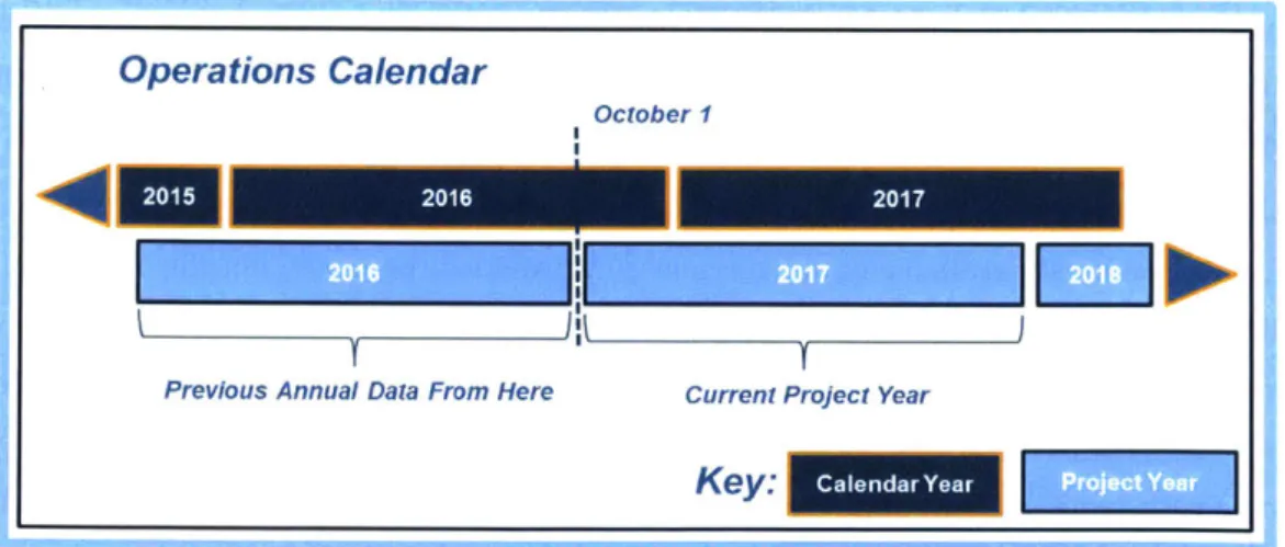
previous project year was assigned. Figure 5 shows a typical operational year, noting that the

weather data is obtained from the previous project year, not calendar year preceding it. For example, Fall weather data for a circuit-year of 2017 is obtained from 2015. This approach assumes that the predictions for the upcoming project year are made at the beginning of that project year. The implication of this method is that for a circuit that is inspected and trimmed late in a project year, for instances August, the data associated will not contain any of the most recent weather that has been encountered since September of the prior year, up to an 11 month gap in the August example. This scheme, despite the late project year issue discussed, was utilized because the model will also be used for planning purposes that are currently solidified before the start of new project year, and would require future weather inputs to be valid.

Operations Calendar

October 1

2015

Previous Annual Data From Here Current Project Year

Key: CalendarYear

Figure 5: Operational Calendar for System Analyzed

Once the weather information for the closest circuit is applied, a check is completed to ensure that all weather parameters were assigned, as it is highly possible that a given weather station

may not have all of the weather variables desired - for example, there may be a station that only

records temperature and not precipitation. If weather variables were not all filled, the next closest weather station is found and any missing values were assigned to the circuit-year. This

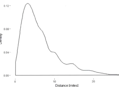
process is repeated until a full weather data frame is obtained. Figure 6 shows the distances for all of the weather stations, note that most weather stations are reasonably close to the circuits, with a mean of 6.4 miles and max of 26.4 miles.

0.12- 0.08- 0.04- 0.00-0 10 20 Distance [miles]

Figure 6: Weather Station Distance Density Plot for 2017 Circuits

Finally, weather data is grouped by season (Fall (FAL): October to December, Winter (WIN): January to March, Spring (SPR): April to June, Summer (SUM): July to September) to limit the number of variables considered in the model. This step was taken to limit the likelihood of collinearities between similar months and additionally shrink the data frame for decreased computational time. This operation decreased the number weather variables from 156 to 39.

2.2.2 Creating Running Average and Standard Deviation Parameters

Previously available data from a circuit provided the model insight into the size of the circuit. Two variables were initially considered: last year's total trims and a running average of prior year's total trims. For modeling, the running average was implemented in favor of the single previous year. Within a single year, there was a significant lag term that presented a source of error with large shifts in units from year to year, which significantly impacted predictions. For the running average a maximum of five previous year total trims was used. When there were less than five years of data available, the running average would take only the available data, for example, for circuit-year of 2004 the running average used only 2002 and 2003 trim information. Although this created circuit years with less than five years running average, the method was implemented with the assumption that including the earlier years in the data set with smaller running averages was better than creating a smaller training set. This assumption was not verified in the modeling conducted.

The same method discussed is used for calculating the standard deviation; however to ensure that the standard deviation was reasonably calculated, three values must have been present. This selection omitted all project years for 2001 and 2002, as 2003 was the earliest that three years' worth of information was available to perform the standard deviation calculation. This variable was not used in general prediction, and is only applied to the model presented in Section 5.4.2 where the normalization is performed on the total trims.

2.2.3 Species Growth Data

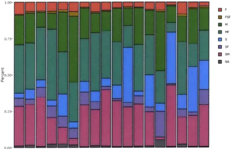
The final manipulated group of parameters is related to species growth data. This process consisted of taking the WMS generated species data from Section 2.1.1 and relating them to the growth rate (i.e. Slow, Medium, etc.) of the individual species. First, all of the species were assigned to a growth rate from their individual species. Next, the percentage of that growth rate making up the circuit was assigned to each growth rate5. Figure 7 shows the distribution of growth rates for 18 of the geographic divisions studied. This method was pursued due to a recommendation in [8] that stated species concentrations was a better predictive variable than land coverage information.

1.00-EF PON FSF M WNW MF 0.75- s 5lF ~ NA C- 20.50- 0.25-0.00-"L L L L L i

Figure 7: Divisional Breakdown of Tree Growth Rate Types

Additionally, the top three species percentage of the total circuit unit count16, calculated in a similar set of steps with growth rate, were also added to the data frame. Percentages were utilized for these variables as a way of clustering similar circuits, but were not included as raw

15 This implies a circuit-year could have, for example, F = 0.625, M = 0.125, and S = 0.250, with the rest

equal to zero.

16 _{An example of the species percentage variable is a circuit that has 25 oak trees, 12 palm trees, 10 birch}

trees, and three other species with 4 trees in a given circuit-year. The highest tree species percentage of the entire circuit, in this case 42%, 20%, and 17% would be reported.

unit values to avoid high correlation with the running average values that are assumed basis for circuit-year scaling.

The rationale behind creating these species variables was related to clustering, where it could be advantageous to group circuits with high concentrations of similar species together. For example, a cluster of fastcircuits could grow at a rate that is independent of weather variables; that is, despite the best trim practices a circuit full of Palm Trees, a Super-Fast species, would need to be revisited annually regardless of the weather conditions. On the other end of spectrum, a circuit compromised of slow growing species might have an increased trim cycle and subsequently might react to long term weather patterns in a unique way. The inclusion of these variables allows for the creation of these type of clusters.

3 Data Exploration

The exploratory data analysis is dedicated to discovering any unique features of the data frame and evaluate any potential useful and/or harmful relationships found within the data. The areas explored include the prediction variable, total annual trims, and the weather data.

3.1 Distribution of Trims

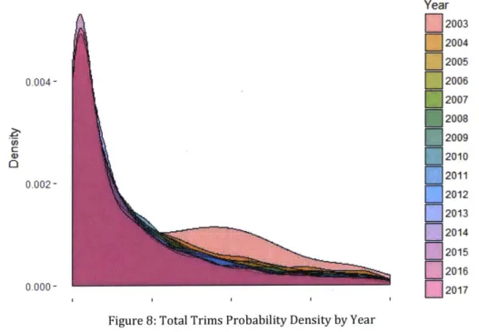
Figure 8 and Figure 9 depict the probability density function for each project years' total trims. Figure 8, a plot of the raw total trims count, shows that many of the circuits in the data frame are skewed to the lower trim count. Figure 9 preformed a log transformation and shows that this transformation creates a nearly normalized circuit distribution. This transformation was not pursued for further analysis due to the fact that the higher unit circuits, which also have higher variances, were challenging to predict in the log form. This was amplified by the face that small log errors were amplified to meaningful raw unit prediction errors that ultimately hinder accuracy metrics. This form of transformation also expands the lower range units further, giving a wider range to values that are practically helpful for accuracy metrics. Lastly, the observed difference in the 2003 distribution can be attributed to only having 82 observations, versus the typical 2,000+ circuits per year.

Year 2003 2004 2005 0.004- 2006 2007

D2008

D

12009

2010 0 2011 0.002- _{2 012} 2013

D2014

D

2015 0.000-

EI2017

Figure 8: Total Trims Probability Density by Year

1 7

A transformation of: log1 0 (TotalTrims + 1) was applied. The addition of 1 was added to avoid issue with

Year 0.8-

D

2003

D

2004 F12005 2006 0.6- 2007

D

2008 Z 2009 0.4- n2010

D

2011 F12012 0.2- 2013 2014 2015 2016 0.0- n.2017

Figure 9: Log Transformation of Total Trims Probability Density by Year

Another transformation investigated was normalization, using the running average and standard deviation. This transformation is shown in Figure 10. This transformation is of interest as it will provide insight into what makes a circuit-year have a number of units above or below a mean year, and thus will evaluate the error from the mean. An interesting observation when the total trims are presented in this fashion is that the center of the distributions are all slightly below 0. For a perfectly normal distribution the errors would be expected to be centered at 0, this tends to imply that there have been a general decrease in the number of units over the years - as the mean value applied is taken from the prior year's averages.

Z-Score of Predictions Year 0.5-2003 2004 - 2005 0.4- 2006 2007 2008 2009 0.3- 2010 2011 2012 2013 0.2- 2014 / 2015 2016 2017

.0-

--5.0 -2.5 0 2.5 5.0

Figure 11Figure 11, an annual boxplot of circuit-year trim, is an attempt to access the prevalence of outliers on an annual basis. The resulting data shows that a large percentage of the circuit-years are classified as outliers. The maximum circuit in a year also appears to be decreasing over the range of years, where 2004 and 2005 contain circuit-years that are roughly two times that 2016 or 2017. Figure 12, a zoomed version of Figure 10, shows a similar trend with the medians and third quartiles deceasing over of the project years.

a * S 0 I * 2

j

S * - S ; I g S * . S - * S 5 S * 2003 E 2004 2005 2006 2007 M 2008 2009 2010 2011 0 2012 F 2013 L 2014 O 201S O 2016 13 2017 2004 2006 2008 2010 Project Year

Figure 11: Total Trims

I

I

I

I

2012 2014 2016

Box Plot by Year

I

I

I

I

* ' S

I.

I

'V 2006 2008 2010 Project Year 2012 2014 2016

Figure 12: Total Trims Box plot by Year without outliers

LU 2003 * 2004 * 2005 * 2006 * 2007 * 2008 * 2009 2010 * 2011 2012 (2 2013 L 2014 0 2015 2016 2017 2004 I

3.2 Weather Data

The investigation of the weather parameters contained three immediate groupings of interest: temperature, precipitation, and drought. Within each of these groups there are focuses to analyze any overarching trends and any collinearities that might exist that would impact variable selection.

3.2.1 Temperature Data

The temperature data contains three general metrics: averages (AVG,MIN,MAX), extremes (EMXT,EMNT), and days (DX90,DT32) in which a weather event has occurred (for example number of days above 90 degrees F). As each of these variables are derived from the same physical phenomena it is expected that collinearity will be present, and as such variable selection prior to model fitting will be required.

Figure 13 takes an initial look at all of the average and extreme temperature parameters via a correlation matrix. Many of the variables appear to be highly correlated, specifically weather variables from the Spring and Summer seem to have the highest correlations. This implies that temperatures from April to June are highly related to temperatures from July to September.

- - WL ii F W W F- F F i W F- F- F- W WU TMAX_WiN TMIN_WI 0.8 TAVGWIN EMXTWIN _0.6 EMNTWIN TUAXSPR _0-4 TMINSPR TAVGSPR _0.2 EMXTSPR EMNTSPR 0 TMAXSUM TMINS -0.2 TAVG SUM EMXT SUM -04 EMNT_-SUM TUAX FAL -0.6 TMIN-FAL -0-8 TAVGFAL EMXTFAL -1

Figure 13: Temperature Data Correlation Matrix1 8

18 Figure 13 is a correlation matrix, where the boxes colors are related to the correlation value between the

Figure 14 explores only the Winter variables, and the same high correlations are seen between the continuous average and extreme variables. Additionally, the days' variables are included and tend to have a lower correlation; however, this is likely an impact of the nature of the variable. For example, in the case of Winter variables, there are probably only a few circuits, if any, that were above 90 degrees F. As a result, it is unlikely that the days variables should be correlated, but for the same reason potentially less insightful for prediction.

zz z z z z z z Z9 9I * ?. I !F.I TMALWI TAVGWIN EMXT.WIN EMNT...WIN DT32LWIN DX32_WIN DX9WIN -0.6 -0.6 ,0.2 60 4.2 64A -4.6 EMXP..VMN -0.32 -.26J-.25 _

Figure 14: Correlation Plot for Winter Temperature Variable19

Boxplots in Figure 15: Boxplot of Minimum Average Temperature by Season and YearFigure 15, Figure 16, and Figure 17, look at few of trends and predominant features of the weather data. Notably in Figure 15 and Figure 16 we observe that many of the box plots for the Spring and Summer seasons appear quite similar, which supports the multiple correlation matrix findings. However, one notable difference between the two different variables in the size of the interquartile range (IQR). In the case of the minimum average variables in Figure 15 the IQR is smaller, especially in the Spring and Summer seasons. Furthermore, Figure 16 does not have as many outliers, once again highlighted in the Spring and Summer seasons. For variable selection this would tend to imply that there is higher variability seen in the Winter and Fall seasons for temperature, which could be helpful for later clustering and modeling predictions. Figure 17 creates a similar boxplot, but for a variable that is preforming a daily count of days with a minimum temperature below 32F within the season. In this variable we notice highly skewed distributions, where in this case Spring and Summer, with exception of one year for the Spring,

19 Figure 14 is a correlation matrix, where the bottom left is the listed correlation value and colored in the

same fashion as Figure 13 (dark red with a correlation of -1 to dark blue with a correlation of +1). The upper right displays the same information where the circles are the size of the absolute value of the correlation (-1 and +1 the largest) and the fill following the same coloring scheme as the bottom left

- -- le_9 0.81082 0.66 0.A9 0.860 -0.32-0.4-0.71 0.79 -0.36 -0.32 -OA1 -0-23 -0.3 0A2 0.26 0 17 0.37

the IQR range is 0 with a median of 0. Although the shape of distributions are slightly different, the correlations can still be high. Combining with Figure 14 we observe that the DT32_WIN has a -0.84, -0.79, and -0.71 correlation coefficient with the average minimum temperature, the average-average temperature, and the extreme minimum temperature respectfully.

70 60 50 40

r

20 * a 0 * 0*0 * HI * 440 Sm a * * S I iS S I I!

II

'S..I U...

.

LI

u;!g;!il. 10

TMINWIN TMINSPR TMINSUM TMINFAL

Variable

Figure 15: Boxplot of Minimum Average Temperature by Season and Year

100 90 80 600 750 60 50

i I

₁

1PIN

0 :1:;,1': --0 .. . .0 -TMAXWIN S * 00 ; ': S. *0

TMAXSPR TMAXSUM TMAXFAL

Variable E IN N U U U 0 rL 03 2003 2004 2005 2006 2007 2008 2009 2010 2011 2012 2013 2014 2015 2016 2017 E 1, U U U U U U U U U 0 0 U U 2003 2004 2005 2006 2007 2008 2009 2010 2011 2012 2013 2014 2015 2016 2017

Figure 16: Boxplot of Average-Average Temperature by Season and Year DT32-WIN 3 0 I. 3. ~ ;1 .310 10 3 3 DT32_SPR DT32 SUM .2 * 3

:

*.': 0 .31.0 0* * * ~ * Ig. *11 .2030 0.00 0*** * 0.03.1 ~ 03 * *~' ~ ~

:;~~

!

*ut

~;.

I;*!

;II

Ii: 'Ii

I:

III

I~

IS

~iw

~:u

DT3LFAL Variable

Figure 17: Boxplot of Days Below 32 degrees F by Season and Year

3.2.2 Precipitation Information

The precipitation data, much like the temperature data, contains three groupings of average, extremes, and daily counts. As noted in the temperature section it is expected that collinearity exists within the data. However, unlike the temperature data the precipitation data is potentially more prone to outlier years of high rains, or extended low rain years.

Figure 18 shows a high correlation among of many of the variables, with the only low correlations found with Summer variables related to the Winter and Fall. This finding indicates that only a single family of precipitation data should be evaluated. Figure 19 looks at the total precipitation for the multiple seasons over the 14 years of the data frame. Within it we see that the low correlations for the Summer season in Figure 18 are attributable to considerably low rainfall in that season on average. Interestingly, the Spring season on average has low median precipitation compared to the Fall and Winter seasons. Lastly in Figure 18, the annual trends within a given season have large variability year to year, a feature not seen in the temperature information. For example, in the Winter season precipitation in 2014 and 2016 are well below and outside of the IQR of the all other years.

80 60 0 E 40 El M U El 1] 2003 2004 2005 2006 2007 2008 2009 2010 2011 2012 2013 2014 2015 2016 2017 20

z z z

0.70-0.75 0.41 0.58 0.4 0.76 0.6110.3 048 0.52 0.39 0.32 0.44 0-3 0.82 0.61 0.5 0.7410.56 0.47 0.65 10.56 0.46 PRCP_WIN EMXPWIN DP01_WIN DP10_WN PRCP_SPR EMXPSPR DPO1_SPR DP10_SPR PRCP_SUM EMXPSUM DP01_SUM DP10_SUM PRCP_FAL EMXPFAL 10.4110.33 DP01_FAL 0.36 DPIFAL 0 3 r .1 0' 1 0.3910.38 0.3310.52 U) 0L 6~ D.79 D.37 J 18 w: a-U1) 0) ,~ (L

n1

0.33 0.27 0.55 0.426.47 0.28 0.49 0.4 .38 0.27 0.27 053 S0.49 0.43 0.53

Figure 18: Precipitation Data Correlation Plot

US I. 5

!1.

;~IIliii

0 PRCP SPR

!IImIajlrnhlaa

PRCPSUM Variable

Figure 19: Boxplot of Total Precipitation by Season and Year

O)l w D U) 0L b. U) I LL₁ 0 a. tr o a-. UiL LLI U-o- ,c 5 C_{a- (} 0 2 U)l a-. 0 wt a-0.91 0.59 0.5310.3610 24

ill

0.461 0.8 0.6 0.4 0.2 0 -0.2 -0.4 -0.6 -0.8 --1

0

_ @4@

4.

0.46 0.3910.84 0.79 0.68 55 0 25 0.25 0.8 0.671 0.55 20 15 S.

II

ii 0S

!

II

* :

10 33_E S 3 UIa; a..

*1

U U U M 2003 2004 2005 2006 2007 2008 2009 2010 2011 2012 2013 2014 2015 2016 2017 0U

:1

5 00 S

I

I

PRCP.WIN

I

PRCPFAL i i i i i i i i i i

e

.

3.2.3 Drought Data

Drought data differs from the preceding variables as it is an externally calculated index, as compared to a distinct measurement. Additionally, the drought indexes have an averaging component that accounts for prior weather information to create the index. Consequently a single extreme precipitation event or warming season, although influential in the other parameters, may not be reflected as strongly in this index. The analysis of the drought indices included: any correlations that might exist between the variables, as there are four potential indices over four seasons to select from, and overall trend information, as it might differ slightly from the previous spot measurement data.

Figure 20 provides the correlation matrix for all drought indices investigated, and shows high correlation among all of the variables. This is interesting as even within the same index the seasonal component does not appear to be unique enough to drive a lower correlation. This finding is potentially related to the nature of the index that takes in historical data and not change drastically seasons by season, resulting in variables that are fairly well correlated.

-IL PDSIFAL PHDIFAL ZNDXFAL PMDIFAL PDSI_WIN PHDI_WIN ZNDX_WIN PMDI_WIN PDSISPR PHDISPR ZNDXSPR PMDISPR PDSISUM PHDI_SUM ZNDX_SUM PMDISUM 0.93 0.62 0.97 0.9 0.92 0.55 0.87 0.84 0.86 -1 j A z z

z af Wr

W W

0

: 2 :

< IL D D D :D a OLLa . 0 7 0 i.4 0. 0 0 . Z . 01 Z 01 T 0. 6- 5- h- a- 8- N 6- 8- ELL L i N a-0.47 __ __ _ 0.97 0.6 0 1*

0.76 0.69

0.82

*

. .

..

*

0.82 0.710.87 0.97 1_ _ _0

0.42

0.38

0.46 0.79 0.77

__

* *

0.75 0.68

0.81

0.980.980.83

**

0.7 0.66 0.77 0.91 0.89 0.77 0.88 0.72 0.66 0.78 0.93 0.92 0.78 0.91 0.98 0.64.4 0.59 . .. 0.65 0.84 0.76 0.7 0.61 0.65 0.71 0.76 0.7 0.92 0.84 0.9 0.81 0.79 0.72 0.9 0.81 0.91 0.88_ 099 1 .9 0.950.92 0.9 0.93 0.82 0.67 0.71 .750. 8810.86 0.74 0.8 0.99 0.97 0.93 0.98 0.97 0.6 0.4810.66

0.580.581

.58]0.430.54I0.73[0.67I0.75f0.68 0.87 0.811 0.79 {065 0.7 0.73 0.86 0.85 0.7310.83

10.98

0.96 0.93

0

0.96 0.99 .99I0.84 - 0.8 0.6 0.4 - 0.2 -0 -0.4 -0.6 -0.8

Figure 21 evaluates the change in Palmer Modified Drought Index over the years of 2003 to 2017. As noted in the precipitation data there were arid conditions in 2014 and 2016, especially in the Winter season. This is seen in the time series of Figure 21where the 2015 and 2016 project years are associated with extreme drought conditions.

6

I

2 E RU -2 -4 -6 -8

LLI ~

q"

:;~

**0

*1

7

I

I!

III

2003 2004 2005 2006 2007 2008 2009 2010 2011 Year

U

(1

*PMDFAL PMDIWIN * PMDISPR * PMDI SUM

I

2012 2013 2014 2015 2016 2017

Figure 21: Boxplot of Modified Palmer Drought Index (PMDI) over Years

I I

U M

I