HAL Id: halshs-00587884
https://halshs.archives-ouvertes.fr/halshs-00587884
Preprint submitted on 21 Apr 2011
HAL is a multi-disciplinary open access archive for the deposit and dissemination of sci-entific research documents, whether they are pub-lished or not. The documents may come from teaching and research institutions in France or
L’archive ouverte pluridisciplinaire HAL, est destinée au dépôt et à la diffusion de documents scientifiques de niveau recherche, publiés ou non, émanant des établissements d’enseignement et de recherche français ou étrangers, des laboratoires
A large scale experiment: wages and educational
expansion in France
Marc Gurgand, Eric Maurin
To cite this version:
Marc Gurgand, Eric Maurin. A large scale experiment: wages and educational expansion in France. 2007. �halshs-00587884�
WORKING PAPER N° 2007 - 21
A large scale experiment:
Wages and educational expansion in France
Marc Gurgand
Eric Maurin
JEL Codes: I2
Keywords: education, returns to schooling, natural
experiment, signaling.
P
ARIS-
JOURDANS
CIENCESE
CONOMIQUESL
ABORATOIRE D’E
CONOMIEA
PPLIQUÉE-
INRA48,BD JOURDAN –E.N.S.–75014PARIS TÉL. :33(0)143136300 – FAX :33(0)143136310
www.pse.ens.fr
CENTRE NATIONAL DE LA RECHERCHE SCIENTIFIQUE –ÉCOLE DES HAUTES ÉTUDES EN SCIENCES SOCIALES
A Large Scale Experiment:
Wages and Educational Expansion in France
Marc Gurgand and Eric Maurin
∗August 24, 2007
Abstract
We evaluate the wage impact of the strong and rapid increase in school-ing levels experienced by the cohorts born after WWII in France. In or-der to identify the causal effect of education, we exploit the fact that the small group of people graduating from elite education (Grandes Ecoles ) remained stable, while the rest of the system experienced tremendous transformation. This provides a well defined control group. Using large scale labor force surveys for the 1990’s, we find that the cohorts that re-ceived more education have a lower wage gap, relative to Grandes Ecoles. We show that such a large scale experiment measures a social return to schooling even in the presence of signaling, whereas strategies based on quasi-experiments are not necessarily robust to signaling. Our instrumen-tal variable estimation finds returns to schooling very similar to the rest of the literature, which is a strong case against the signaling hypothesis.
1
Introduction
As a result of renewed interest for education policies and evaluation methods, significant progress has been made over the past decade in the measure of re-turns to schooling. Convincing figures mostly confirm the picture based on traditional Mincerian wage regressions: that returns to schooling are about 8% in developped countries, maybe slightly higher (see Card, 2001, for a survey). They result from empirical strategies based on quasi-experiments: exploiting a source of exogenous variation in individual schooling levels allows to identify the causal effect of education on wages. Typical examples are Angrist and Krueger (1991) that use quarter of birth as a random event or Oreopoulos (2006) using a regression discontinuity design.
∗Gurgand: Paris School of Economics / Paris-Jourdan Sciences Economiques (UMR 8545
CNRS-EHESS-ENPC-ENS) and Crest; Maurin: Paris School of Economics / Paris-Jourdan Sciences Economiques, CEPR and Crest. Email: gurgand@pse.ens.fr, maurin@pse.ens.fr. This paper has benefited financial support from the CEPREMAP Public finance and redis-tributive policies program. We thank seminar participants at Crest, Université catholique de Louvain and Iredu.
Some of these approaches jointly provide returns to schooling estimates and the evaluation of schooling policies: for instance Duflo (2001) for school building in Indonesia, Meghir and Palme (2005) for secondary education reform in Swe-den or Oreopoulos (2006) for compulsory schooling laws in the United Kingdom. However, evaluation requires that these policies be local, either in the geograph-ical or cohort dimension. Yet, many policies are general and long lasting, such as the comprehensivation of the British system or the French democratization considered here: it is no less important to measure their consequences in a convincing manner.
Moving away from the canonical experimental paradigm has another feature: it is less likely that returns to schooling can result from mere ability-ranking. Indeed, since the 1970’s, the possibility that the value of schooling may lie in its informational content rather than result from improved productivity (the so-called signaling model), has been a serious theoretical challenge to the hu-man capital literature. In a hypothetical controlled experiment, whereby a few randomly chosen individuals would be granted more schooling, their wage in-crease would actually be caused by education. However, in a pure signaling model, they could simply free-ride over the signal conveyed by the mass of educated individuals that are, in equilibrium, the most intrinsically productive ones. Therefore, such a convincing identification strategy would measure private returns but would fail to measure social returns - thus would have ambiguous policy implications - if signaling played a role in the labor market.
Recent empirical evidence over the signaling model is limited and mixed (Lang and Kropp, 1986, Kroch and Sjoblom, 1994, Bedard, 2001, Chevalier et al., 2004, for instance). Therefore, the policy implication of estimated returns to schooling remains an open question, and one that is rarely raised in the recent literature. Large scale experiments allow to make progress in this direction, be-cause a general wage increase resulting from wide educational expansion cannot result from mere ability-ranking among the population. Naturally, this must come at the cost of less random-like identification strategies.
In this paper, we evaluate the strong and rapid increase in schooling levels that affected the cohorts born in France between 1946 and 1970. During this period, the share of males with no degree dropped from 43% to 25%, whereas school duration increased by 2.5 years on average. This has been a complex process, involving more schooling, to a large extent focussed at vocational ed-ucation, but also a progressively less segmented secondary education system. We evaluate the male wage impact of this experience as a whole. In particular, we compute returns to schooling that, we argue, do not include private returns from signaling, if any. The returns we find - 5 to 9% - are very similar to the rest of the literature and, as often, slightly higher than standard OLS estimates. As such, these findings are not supportive of the signaling model, and it is very likely that private returns provide a legitimate guidance for policy purposes.1
Our evaluation of the French experience relies on the existence of a control
1In a very different setup, Acemoglu and Angrist (2000) cannot find positive externalities
deriving from average schooling in the population, which implies similarly that private returns are no different from social returns.
group: the male population that receives elite education in the very traditional Grandes écoles system. It hardly changes in size (4%) and composition over this period: we thus assume that the unobserved characteristics of this group remain constant, relative to the 96% remaining population. Using a difference-in-difference approach, we can trace out the wage gap between the Grandes écoles graduates and the rest of the population, accross cohorts observed in the same labor market - that of the 1990’s. As the latter group becomes more and more educated, the wage gap should decrease if schooling increases wages. More-over, this cannot result from mere signaling, as it cannot result from relative positions within the 96% "treated".
The rest of the paper is organized as follows. Using a canonical signaling model, Section 2 clarifies the conditions under which schooling returns based on quasi-experiments can measure social returns if the signaling model is relevant, and argues that the current approach is robust in this sense. Section 3 presents educational expansion in France over the period considered and the specific situation of Grandes écoles. The identification strategy based on difference-in-difference and instrumental variables is exposed in Section 4 and results are presented in Section 5. Finaly, Section 6 explores the possibility that the results could be driven by the evolution of the minimum wage. Section 7 concludes.
2
Human capital vs.
signaling : interpreting
returns to schooling
From a policy perspective, the labor market signaling model introduced by Spence (1973) challenges the literature on returns to education. This model argues that wage-education contracts can be rationalized as a separating device that reveals unobserved productivity to employers (see Riley, 2001, for a general exposition). As a result, the wage-education relationship does not necessarily imply that schooling raises productive capacity. Social and private returns to educational investment then differ. This section clarifies the conditions un-der which returns to schooling estimated using quasi-experiements are likely to measure social returns, if the signaling model is relevant. It illustrates that an empirical strategy based on a full scale experiment, like this one, is very likely to measure the full social returns to education in all cases.
Consider an economy with one schooling degree and initial productive capac-ity u continuously distributed in the population, with cumulative F (u). Individ-uals can undertake education at a cost c(u) that is decreasing in u and education enhances productivity by β ≥ 0. Call w0(u) the wage received by an individual with productivity u and no degree, and w1(u) her wage if she receives education. The optimal choice is always to choose education if c(u) ≤ w1(u) − w0(u).
We consider two opposite models. In the human capital model, individuals are paid their own marginal productivity, so that:
w0(u) = u w1(u) = β + u
We specify the signaling model in a way similar to Bedard (2001). If a separating equilibrium exists2, it is such that:
c(u∗) = w1(u∗) − w0(u∗)
where u∗ is the marginal type that chooses to receive education, with:
w0(u∗) = E(u|u ≤ u∗) (1)
w1(u∗) = β + E(u|u ≥ u∗)
In essence of the signaling model, workers are paid the average productivity in their group.3
The typical quasi-experimental strategy to estimate returns to education does identify private returns to education, holding down unobserved ability, but it may fail to estimate the same parameter in either model. Consider an experiment or an instrumental variable that randomly lowers the schooling cost for a share α of the population: individuals thus treated (T = 1) face a cost ec(u) < c(u). Call u∗ and ue∗ the marginal types in the untreated and treated population respectively. The corresponding shares of unschooled individuals are F (u∗) and F (ue∗). The Wald estimator used in the quasi-experimental approach is based on the comparison of treated with untreated, namely:
E(w|T = 1) − E(w|T = 0) [F (u∗) − F (eu∗)]
In the human capital model, the reduced form difference is:
E(w|T = 1) − E(w|T = 0) = [1 − F (eu∗)] β + E(u) − [1 − F (u∗)] β − E(u) = [F (u∗) − F (eu∗)] β
so the Wald estimator measures β, which happens to be both the social and the private return in this model.
In the signaling model, provided that the employers cannot identify the treated from the untreated, which would be typically true in a small-scale experiment or if information on wether a person is under treatment is not readily observable, wages are now formed as a mixture of treated and untreated average produc-tivity in each schooling level. Assuming a separating equilibrium exists, the marginal types in each population are such that:
c(u∗) =ec(eu∗) = w1(u∗,ue∗) − w0(u∗,ue∗) with equilibrium wages set at:
w0(u∗,eu∗) = F (eu∗)E(u|u ≤ eu∗) + (1 − α) [F (u∗) − F (eu∗)] E(u|eu∗≤ u ≤ u∗) F (eu∗) + (1 − α) [F (u∗) − F (eu∗)] w1(u∗,eu∗) = [1 − F (u ∗)] E(u|u ≥ u∗) + α [F (u∗) − F (eu∗)] E(u|eu∗≤ u ≤ u∗) [1 − F (u∗)] + α [F (u∗) − F (eu∗)] + β
2We do not discuss here the conditions for existence and unicity. We simply consider the
possibility that there is signaling in the economy and the implications this would have for estimation methods.
3Empirical wage heterogeneity within schooling levels is not modelled here and could result
Comparing wages of treated and untreated now gives:
E(w|T = 1) − E(w|T = 0) = F (ue∗)w0(u∗,eu∗) + [1 − F (eu∗)] w1(u∗,ue∗) −F (u∗)w0(u∗,eu∗) − [1 − F (u∗)] w1(u∗,eu∗) = [F (u∗) − F (eu∗)] [w1(u∗,eu∗) − w0(u∗,eu∗)] and the Wald estimator thus measures:
E(w|T = 1) − E(w|T = 0)
[F (u∗) − F (eu∗)] = w1(u∗,ue∗) − w0(u∗,ue∗) > β
The signaling effect of education is captured altogether with direct productivity effect. In particular, a positive private return can be found, even when β = 0.
Notice also that, in this model, the quasi-experimental approach would be strictly equivalent to ordinary least squares. This could provide another possible interpretation to the fact that instrumental variable estimates are only slightly higher than ordinary least squares in most empirical applications (Card, 2001): the small rise could simply be due to measurement error correction in the ab-sence of a more foundamental difference. Our results, however, will rule this out as a serious line of interpretation.
The center piece is that a quasi-experimental or instrumental variable strat-egy is robust to the signaling hypothesis only if we can assume that employers can sort out treated and untreated. The ideal controlled experiment that would draw randomly a small sample of persons would identify private returns per-fectly, but would fail to demonstrate the existence of a social return. In contrast, an empirical approach based on a full scale policy that affects entire generations is more robust to the possibility that there is signaling. In such an experiment, treated and untreated can be sorted out by employers, as they well known that schooling distribution has evolved and that degrees held by younger people may mean less. An interesting implication is that robustness to signaling may come at the cost of a weaker identification strategy.
The experiment considered in this paper can be viewed as a decrease in schooling cost from c(u) to ec(u) < c(u) over two generations, which leads to a general schooling level increase in the second generation. The central point is that generations are sufficiently far appart that employers are very aware of their potential differences, in particular regarding their unobserved ability. The second generation being the treated one (T = 1), it is trivial that the Wald estimator measures β in the human capital model. In the signaling model, the first generation receives w0(u∗) and w1(u∗) as defined in equation 1 whereas the second generation receives w0(ue∗) and w1(ue∗). However, the Wald estimator still measures β: E(w|T = 1) − E(w|T = 0) = F (ue∗)w 0(eu∗) + [1 − F (eu∗)] w1(eu∗) −F (u∗)w 0(u∗) − [1 − F (u∗)] w1(u∗) = [F (u∗) − F (eu∗)] β
The intuition is very obvious: as long as the mean E(u) is the same in the two populations, an increase in average wage can only result from the real impact
of schooling, β. Obviously, large scale experiences bring more information on social returns than do small scale experiments. As a corolary, the signaling model can be ruled out if returns are insensitive to the size of the experiment used for identification.
With generations far appart, however, we cannot exclude systematic differ-ences in mean productive capacity accross cohorts. This would be confounded with the effect of schooling, β. In our empirical setup, therefore, we introduce "Grandes Ecoles" (thereafter GE) to control for these potential changes. In the context of this illustrative model, GE would come as a third level, rationed by a numerus clausus, so that the specific cutoff type u for GE does not change accross generations. The data examined in the next section show that this is a reasonable assumption. As a result, we can interpret changes in average GE wages between generations as a measure of cohort-specific changes rather than changing selectiviy into that level. This provides a control for systematic differences in unobserved ability accross cohorts.
3
Educational expansion in France
The cohorts born after World War II in France have experienced a strong and rapid increase in schooling levels, only comparable to the generalization of pri-mary education that occurred in the late 19th century (Marchand and Thélot, 1997). Two phases can be distinguished. The first one concentrated efforts on vocational education, especially at secondary education level: it implied cohorts born from 1946 until the mid sixties. The second phase witnessed a fast in-crease in high school graduation for cohorts born from the mid-sixties to the mid-seventies.
In order to document this evolution, we use data from the French labor force surveys (enquêtes Emploi ) from 1990 to 2002. This data is a yearly rep-resentative sample of 1/300 of the metropolitan population, in which schooling information is very detailed. We restrict our sample to individuals aged 26 to 56 (and out of school) at survey date. Because the survey has a three years rotating panel structure, we use only one out of three years in order to compute the cohort schooling levels, so as to exploit information on a single individual only once. When we get to estimating wages, we will use the same data, but with all available years and make proper adjustment to estimator variances for individual correlation over time.
3.1
Two periods of a fast increase in secondary education
As illustrated by table 1, the main target during the first phase was lower sec-ondary school, with specific emphasis on its vocational components4: about 30% of men born in 1946 had one such degree and this figure rose to 38% twenty years later. For women, the figures are 21% and 30% respectively. Meanwhile, the share who ended up with no degree at all from initial education decreased from43% (for men) and 53% (for women), to 30% (for men) and 28% (for women). This trend is due to reforms that have made access to lower secondary educa-tion easier and more democratic. During that period, the effort on vocaeduca-tional schooling also took place at a higher education level (grades "Brevet de techni-cien supérieur " and "Diplôme universitaire technologique", both lasting for two years after High School): the share of a cohort with such degrees increased from 5% to 9% for men and 6% to 12% for women. This resulted from the increased supply (in volume and diversity) that took place in the late 1960’s.
The second phase was shorter but faster: over ten years (individuals born from the mid-sixties to the mid-seventies), the share ending up with no degree decreased by an additional 8 percentage points, and the share at lower voca-tional education also decreased, whereas access to higher vocavoca-tional education continued to rise, by about 5 percentage points for both men and women. More importantly, the share of the population getting a High School degree ("Bac-calauréat ") increased at an unprecedented pace: it doubled from 11 to 22% for men and rose from 15 to 24% for women. To a large extent, this increase was due to technical High School curricula, so that, overall, long term vocational training has been substituted for short term one over this period. It should be noted that the share of a cohort getting a Baccalauréat degree (or higher) is stable since the mid 1990’s (that is for cohorts born after 1975 approximately). To sum up, during the first period (twenty cohorts), average declared school-ing duration increased by 1.4 years for men and 1.9 years for women (from 11.3 and 11.1 years, respectively). The second phase was even more impressive: over only ten cohorts, average schooling increased again by 1.6 years for both men and women.
3.2
Grandes écoles and higher education
While such strong changes were taking place, little or very little was happening at higher education levels. In table 1, we have broken down non-vocational higher education into three levels: the first level is a University two-years degree, corresponding to the American Colleges; the second level is University Graduate level, up to PhD. The third level is specific to the French two-tier system. Since the early 19th century, a higher education track, distinct from University, developped in parallel, under the label Grandes écoles. They form an elite sector, with rationed entry, ruled by selective examinations. The students from High School considered the most academically performant are accepted into two-years "Classes préparatoires", where they are trained for this examination. Depending on their ranking, they are then received into the clearly stratified GEs, where training lasts two to three years. Those who fail the selective examination join University at the Graduate level. GEs are traditionnally public and train mostly engineers, but private management schools are also present.
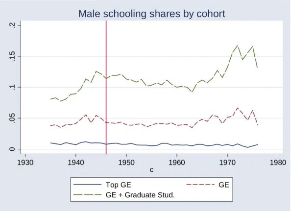
From table 1 and figures 1 and 2, it is apparent that the share of a cohort getting any of these three levels as a highest degree hardly changed during the first phase defined above, and this is in sharp contrast with what happened in the rest of the schooling system.
This observation will be the basis for our empirical strategy. As access to GE is a rationed process that has not expanded, it is reasonable to assume that, year after year, it was attended by the "same" population: the 5% most successful students. This provides us with a control group, whose unobserved characteristics (specifically "ability") has not changed relative to the rest of the population. In another context, a related identification strategy has been used by Acemoglu and Pischke (2001), who assume rank in the income distribution to be a proxy for the household unobservable characteristics that affect demand for schooling, and could be counfounded with income level.
In a nutshell, if educational expansion affecting the bunch of the population has a causal effect on wages, then the cohort-based wage gap with those who access GEs must have decreased. Such a decrease cannot result from unobserved characteristics.
Strictly speaking, however, the share of GE appears to be constant for men belonging to cohorts 1946-1964 (see tests in table 2), that is during the first phase of educational expansion. The male cohorts 1964-1973, as well as females over the whole period, experienced a slow but statistically significant increase. When we isolate the Top ranked GEs (that represent about 20% of GE students5), the share is also constant for the cohorts 1946-1964, and even so for a larger span, 1946-1970. In contrast, if we enlarge the GE group to include Gratudate studies, the share moves significantly with cohorts, even for males, first decreasing, then increasing.
In the following, we will thus consider two definitions of the "control group", GE or Top ranked GE, the latter for both cohorts sets 1964 and 1946-1970. Also, in order to avoid issues related to labor supply and selectivity, we will restrict our wage analysis to males.6 As illustrated in tables 1 and 2, the wage earners sub-sample shares the features of the whole population.
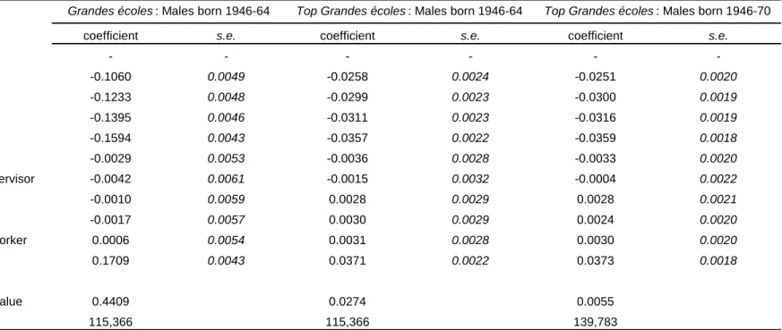
In order to justify further the hypothesis that the GE group maintained a stable composition relative to the population, we test that its social origins did not change. The labor force surveys have information on the father’s profes-sion. Using five social classes, in order to have sufficient data, table 3 regresses the probability to be a GE or Top-GE graduate, conditional on social origin, a cohort trend and a cohort trend interacted with social origin. The social stratification is very clear, but, for GEs, it does not change significantly over time (the same holds for the wage earners sub-sample). Albouy and Wanecq (2003) have made a comparable statement using the same data. The hypothesis seems less robust for Top-GEs: sons of modest origin tend to catch up with sons of managers, whereas the intermediate class tends to loose ground. However, these movements are very small. Furthermore, Euriat and Thelot (1995) have analyzed exhaustive data on the four most prestigious Top-GEs: Ecole poly-technique, Ecole normale supérieure, Ecole nationale d’administration (ENA) and Hautes études commerciales (HEC). They find that, for our period of in-terest, the students’ social origins, relative to the social structure of the whole
5The list of Top GEs is imposed to us by enquête Emploi.
6If anything, the fact that women access to GE has increased over cohorts would imply
population, has remained remarkably stable.
4
Empirical model and identification strategy
4.1
The difference-in-difference model
Consider the following wage equation:
log w = θc+ γa+ βd+ u
where c is an index for birth cohort, a for age, d for schooling degree (starting d = 1 for no degree, up to d = n for the highest) and u unobserved productive capacity. As date effects cannot be separated from age and cohort effects, they are embedded in parameters θc and γa, that have thus no direct interpretation. This model is additive in age, following the recent literature (e.g. Duflo, 2001, Meghir and Palme, 2005, Oreopoulos, 2006, etc.) that relies on cohort analysis to estimate returns to schooling.
Wage expectancy conditional on schooling, cohort and age is: E(log w|d, c, a) = θc+ γa+ βd+ E(u|d, c)
Expectancy E(u|d, c) varies with schooling d both because schooling decisions are endogenous and because the schooling system is selective: this is the so-called "ability bias". This expectancy also varies with cohorts c because, as access to some degrees is enlarged or restricted, the average ability of the population with any level d may change. For that reason, variations in schooling levels accross cohorts cannot be used directly as a source of identification for parameters βd. Yet, the identification strategy pursued in this paper relies on the observa-tion that the share and social structure of the populaobserva-tion receiving the elite degree d = n ("Grandes écoles") remained stable over several cohorts, whereas huge changes were taking place in the rest of the schooling system. Therefore, we assume that selectivity between that level and the rest of the population remained constant accross cohorts, in the sense that:
E(u|d < n, c) − E(u|d = n, c) = E(u|d < n) − E(u|d = n), ∀c (2) This provides a control group for difference-in-difference identification. For the upper level:
E(log w|d = n, c, a) = θc+ γa+ βn+ E(u|d = n, c) Also, for the group that did not get d = n:
E(log w|d < n, c, a) = θc+ γa+ X j<n
Comparing average GE wages with that of the rest of the population defines ∆(c). Under (2): ∆(c) = E(log w|d < n, c, a) − E(log w|d = n, c, a) = X j<n βjP (s = j|d < n, c) − βn+ E(u|d < n) − E(u|d = n) A difference-in-difference estimator thus identifies:
∆(c0) − ∆(c) =X j<n
βj[P (d = j|d < n, c0) − P (d = j|d < n, c)]
Because the share getting a given degree rises with cohorts at all levels (except ”no degree”), the difference ∆(c0)−∆(c) must be positive for c0> c, if it is the case that rising education increases wages (namely: β1< β2< . . . < βn). As such, the wage gap between GE graduates and the rest of the population taken as a whole must decrease, as the general schooling level rises (even though the level of selectivity may change over time for any degree d < n). Note that this does not exclude the possibility that E(u|d = j, c) decreases along cohorts for every j < n, as a result of expanded access of each level to students with lower academic performance.
Notice that P (d = j|d < n, c) is observable, so that in principle, all βj’s could be identified separately. Unfortunately, over the period considered, those probabilities move in parallel, so that the contribution of each schooling level is not distinguishable empirically. The parameter that we can actually estimate instead provides a general assessement of twenty years of educational expansion, which is not disaggregated, but is very robust under hypothesis (2).
The model is estimated based on the following specification:
log w = θc+ γa+ α1(d < n) + bc1(d < n) + ε (3) with 1(d < n) a dummy for non-GE graduate. Normalizing b1946 = 0, for instance, bc would estimatePj<nβj[P (d = j|d < n, c) − P (d = j|d < n, 1946)] that must be positive if there is a return to education. Parameter α estimates E(u|d < n) − E(u|d = n) − βn, that is the baseline wage gap between GE and the rest of the population, including the effect of unobserved characteristics, which cannot be distinguished from the causal effect βn.
4.2
Instrumental variable estimation
The core hypothesis in this paper is that a change in the differential wage between GE graduates and the rest of the population accross cohorts can only be explained by educational expansion. In order to quantify this effect in terms of return and compare orders of magnitude with the literature, we can correlate the drift in bc with the increase in average schooling years (below level n) by cohort. More formally, we can switch this approach to an instrumental variable strategy. Consider the equation:
where S is an individually defined variable that measures schooling time.7 The difference-in-difference model assumes that the interaction between cohort dum-mies and no-GE dummy, explains education but has no direct effect on wages, once no-GE dummy and cohort dummy are included additively in the model. As a result, the set of interactions provides a vector of instrumental variables for S.
This approach does not imply that we have to assume a constant mar-ginal return to schooling time, r, accross education levels or accross individ-uals. Rather, the IV estimate can be interpreted as a weighted average of possibly heterogenous returns, what Angrist and Imbens (1995) call an aver-age causal response (ACR). To be explicit, take cohort 1946 as a reference, consider cohort c and the instrument Zc = 1(d < n) × 1(cohort= c). Specify log w = θc+ γa+ α1(d < n) + RS + u, where RS is a counterfactual individ-ual specific shift associated with S years of education. For IV to estimate the ACR, two assumptions are needed. First, the monotonicity assumption that moving from cohort 1946 to cohort c would never imply reduced schooling for anybody. Second, the independance assumption that the instrument is orthog-onal not only to counterfactual wages at any level S, but also to the sequence of schooling responses to the instrument itself. Under these conditions, the IV parameter r (based on the two cohorts only in this example) estimates:
X k
ωkE [Rk− Rk−1|S1≥ k > S0]
where S0is counterfactual schooling for Zc = 0 and S1is counterfactual school-ing for Zc= 1 and:
ωk=
P (S1≥ k > S0) P
jP (S1≥ j > S0)
is a weighting factor. Rk− Rk−1 captures the local return at schooling duration k. The condition S1≥ k > S0 implies that only individuals who would increase their education under the effect of the instrument contribute to the estimation. Moreover, the education levels at which changes are more likely make a stronger contribution. The monotonicity assumption, that allows such an interpretation, is reasonable in this context: it implies that the increase should take place at all education levels (except GE) along cohorts, which we actually observe. The independance assumption basically requires here that, if cohort 1946 had been exposed to the cohort c schooling system, it would have had the same schooling levels on average.
When more cohorts are included, the estimator measures a weighted sum of these effects, where cohorts that contribute a more efficient estimation receive more weight (see Angrist and Imbens, 1995, theorem 2).
7Notice that, as we condition on age rather than on potential experience, the return that
we estimate takes into account the fact that an additional schooling year reduces potential experience by one year. In that sense we compute net returns. They should be lower than the returns based on traditional Mincer equations, but are more policy relevant and are comparable to much of the returns estimated in the recent literature.
5
Estimation results
5.1
Difference-in-difference estimation
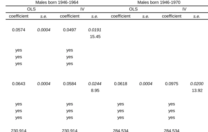
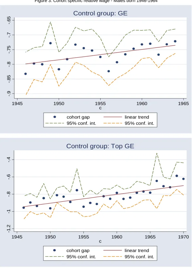
Equation (3) is estimated based on data on males aged 26 to 56, from the 1990 to 2002 labor force surveys enquête Emploi, using the hourly log-wage rate as an explained variable. As individuals are surveyed three years in a row - following a rotating panel structure - we allow for panel individual autocorrelation. Figure 3 presents the series of estimates of the cohort wage gap between GE and non-GE, (α + bc) defined in equation (3), for several definitions of the control group over the samples 1946-1964 and 1946-1970. It shows very clearly that the wage gap between GE graduates and the rest of the population is decreasing along cohorts, for both control groups and samples. Assuming that the differences in unobserved ability accross the two groups did not change, we can interpret this as the result of the strong increase in the schooling level of the "treated" group. Figure 3 also shows that the evolution of cohort effects is reasonably approx-imated by a linear trend. The corresponding specification is presented in table 4 for the two samples and GE or Top-GE when applicable. Specification (1) im-plies that the wage gap between GE students and the rest of the population has decreased by about 0.35% per generation, or about 6.3% in all 18 generations.8 During this first shooling expansion period, the share of the male population with some degree increased by 14% (table 1). Therefore, the average degree was worth a 45% wage increase (0.063/0.14).
The effect is somewhat higher when we consider Top-GEs and when we ex-tend the cohort range. The wage gap reduction rises up to 1% per generation. This trend in wage gap reduction is all the more striking, as school duration increased slightly for GE graduates over the period (see table 1). An obvious reason for these higher figures is the accelerated increase of schooling level that took place during the second period of educational expansion. In addition, as we extend the cohort range, the very nature of schooling progress changes. In-deed, during the second period, about 22% of the population has shifted from no degree or lower vocational degree to High school graduation or tertiary voca-tional degree (table 1). These maybe more rewarding degrees, or the population concerned by these very changes may have higher latent returns to schooling than the population affected by the increase at lower secondary education, that characterized the first period. Generally, one must bear in mind that this is an overall evaluation of a set of actions that resulted in increased levels but included many qualitative changes and a complex intrication of schooling policies.
5.2
Instrumental variable estimation
Relating the above cohort trends with the corresponding increase in schooling duration provides a measure of the returns to schooling that would make this
8This figure is not directly apparent in the table because the cohort variable has been
results comparable to the literature. Equivalently, instrumental variable estima-tion of the standart returns to schooling model are presented in Table 5, using the declared age at completed initial education to measure schooling time. Or-dinary least squares are also reported. The OLS returns are around 6%, which is very much in line with what is usually found in developped countries.
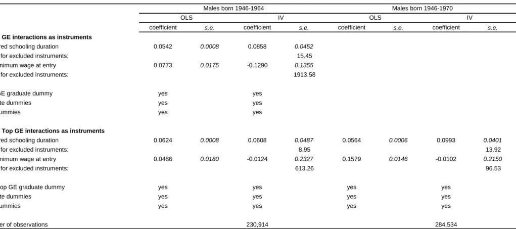
The IV estimates use either GE dummy interacted with cohort dummies or Top-GE dummy interacted accordingly. For the base sample, 1946-1964, they are slightly lower, between 5 and 6%, depending on the set of instruments. This should not result from weak instruments that would bias the IV estimator towards OLS, because the excluded instruments explain schooling duration very well. The estimation based on the extended cohorts generates a somewhat higher return (9.8%), but it is not significantly different from the OLS at the 5% level. As discussed in the above section, the nature of the educational expansion for the additional cohorts 1965-1970 is specific: the reduced form has shown that, when these cohorts are included, the cohort effect is somewhat steeper. Using different identification strategies, Maurin and McNally (2005) and Maurin and Xenogiani (2007), find very comparable results for France.9
In theory, there is a possibility that selectivity could drive those results: the younger low education cohorts could be more often unemployed, so that the productivity of the working sample could be higher than for older cohorts, if the unemployed are on average less productive. Yet, the 26-56 age range is not the most sensitive to unemployment. Moreover, selectivity correction can be implemented using the GE×cohort interactions as instruments for both schooling and selection probability, because there are as many as there are cohorts. When we introduce the selection probability as a control function in various ways (as an inverse Mills ratio or as a quartic function), returns to schooling remain very robust.
Overall, these results are very much in line with the previous litterature that uses IV based on quasi-experiments to estimate the returns to schooling. In most of the available estimates, OLS returns are most often around 6 or 7% and incrase slightly - but not always - when IV is implemented (cf. Card, 2001, table II). In most cases, the difference between OLS and IV are not significant. As argued, our estimation based on a large scale experiment should be more robust to the possibility that the underlying model involves signaling, so that this 5 to 9% coefficient can be considered a measure of the social return to schooling. There is no evidence that this return is very different from either OLS in France or estimates elsewhere based on strategies that would measure the private rather than the social return if they were distinct. In this context, there is little evidence in favor of the signaling hypothesis.
9More precisely, those two papers report returns to the order of 13-14%. But this paper
measures years of education as actual duration spent studying, including grade repetition, whereas the above mentioned papers use years implied by attained levels. Using the latter measure here would generate returns around 10-13%. The difference between our baseline 6-9% and this 10-13% indicates how much is spared by frequent repetition in the French system.
6
The minimum wage impact on wage
equaliza-tion
In assumption (2), E(u|d < n, c) and E(u|d = n, c) are understood to describe the evolution of the unobserved characteristics of individuals, that may affect simultaneously school performance and the wage rate. We have argued that it is a reasonable hypothesis, in the French context, to consider that E(u|d < n, c) − E(u|d = n, c) is constant accross cohorts 1946-1964 or 1946-1970 (depending on the definition of n). As a result, we attribute changes in the wage gap, as depicted in figure 3, to the increased schooling level of the treated group. But we may consider that labor market or other events also contained in the residual u, could equalize wages along the cohort dimension. In this section, we explore the possibility that the minimum wage could have such an equalizing effect, if workers at lower schooling levels have benefitted from minimum wage increases. Figure 4 shows the strong movements in the (net) minimum wage that occurred since WWII, whether expressed in real terms or relative to the average wage.
First, notice that the current level of the minimum wage is not a source of concern. As cohorts get more educated on average, they should be less affected by the minimum wage truncature, conditional on age: by itself, this would predict an increase in the wage gap, rather than the observed decrease. However, conditional on age, different cohorts are not observed at the same date, therefore at the same level of the minimum wage. Yet, as illustrated in figure 4, the minimum wage was fairly stable during the 1990’s, our period of observation. All in all, current minimum wage is not an obvious alternative explanation to our findings.
The impact of past minimum wage could be more relevant, to the extent that entry wages have lasting effects. Baker et al. (1994) argue that this is the case in the United States. In the same line, Beaudry and DiNardo (1991) find a link between past unemployment and current wage, although von Wachter and Bender (2006) argue the evidence is not so strong. Still, there is no available evidence for the minimum wage impact specifically. If there is persistency, then a wage increase (relative to GE) accross cohorts could be explained by a trend in the minimum wage at the time of entry in the labor market. For cohorts 1946-1964, the relevant minimum wages are those prevailing between 1959 and 1990. Over this period, the minimum wage was first stable (or decreased relative to the average wage), then increased strongly, then was stable again (figure 4). To test whether the minimum wage is an omitted variable in the previous estimations, we include it, evaluated at time of entry on the labor market. Our initial equation is thus extended to:
log w = θc+ γa+ α1(d < n) + rS + λwc+6+S+ ε0
where wtis the minimum wage at date t and c + 6 + S measures age at entry on the labor market. It is important to note that, because schooling is endogenous, so is wc+6+S. A higher minimum wage due to longer schooling and thus later entry, may be confounded with unobserved ability. We can instrument this
variable using the same instruments as previously, because there are as many instruments as there are cohorts. Identification is made possible because the schooling variable is increasing steadily with cohorts, whereas the minimum wage is stable for early and late cohorts.
Results are presented in table 6, with the real minimum wage included in levels. Based on ordinary least squares, entry minimum wage seems to have some effect on future wages, but this has no impact on the estimated returns to schooling in any specification. Once schooling and minimum wage are in-strumented, there is no longer any evidence that the latter has some impact, whereas the IV returns to schooling remain similar to previous results, or even slightly higher but also less precisely estimated.
Another approach is to leave out the workers with low education, say less than S = 10, thus those most affected by the minimum wage.10 If minimum wage changes were driving the results, the returns to schooling should drop. If we do this, however, the "treated" population is no longer stable accross cohorts: as general education levels increase, individuals with a given low schooling level represent a smaller and smaller share of the population. Should they be in the lower tail of productive capacity, the remaining group (S ≥ 10) would have decreasing average unobserved productivity. Therefore, if anything, we would underestimate the returns to schooling. The corresonding IV estimates are presented in table 7. Coefficients are similar to baseline IV, with only an increase for cohorts 1946-1964 with GE as a control group, but not a significant one, given confidence intervals. Overall, we can find no convincing evidence that the minimum wage does explain the constant trend in wage gap reduction.
7
Conclusion
This paper uses a difference in difference strategy to evaluate a large scale policy: the significant and fast increase in schooling levels that benefited the cohorts born after World War II in France. It exploits the fact that the group that had access to the elite segment of the educational system, the Grandes écoles, has remained stable in size and social composition. As a result, the evolution of the wage gap between GE graduates and the rest of the population, cohort after cohort, should reflect the fact that the schooling level of the "treated" group has increased steadily relative to the "control", and should not result from changes in their relative unobserved characteristics. Using labor market data for the 1990’s, thus observing every one in the same economic environment, we find indeed that the wage gap has become regularly and significantly smaller cohort after cohort. Quantifying this effect implies wage returns to schooling between 5 and 9%, in the usual range for developped countries.
Naturaly, there can be other events that, for some cohorts and not others, affected GE graduates differentialy from the rest of the population. In par-ticular, we explore the possibility that increased minimum wage over much of
1 0The S = 10 threeshold is used because a large share of increased schooling under the
the period when these cohorts entered the labor market, could explain the gap reduction. Our results are robust to this possibility.
Although our identification strategy is not based on a quasi-random feature, it offers an evaluation of a large and long lasting experiment taken as a whole. Moreover, the interpretation of returns to schooling is straightforward in such a setup: steady wage increases of entire cohorts is not compatible with the view that there are private but no social returns to schooling. As our estimated returns are similar both to ordinary least squares and to returns estimated elsewhere, it is likely that there is little gap between private and social returns in general. This is a strong case against the signaling hypothesis.
References
Acemoglu D. and Angrist J., 2000, "How large are human capital externali-ties? Evidence from compulsory schooling laws", NBER Macroannual, 9-59.
Acemoglu D. and Pischke J.-S., 2001, "Changes in the wage structure, family income, and children’s education", European Economics Review, vol. 45, 890-904.
Albouy V. and Wanecq Th., 2003, "Les inégalités sociales d’accès aux grandes écoles", Economie et statistique, n◦361, 27-52.
Angrist J. and Imbens G., 1995, ”Two-stage least squares estimation of average causal effects models with variable treatment intensity”, Journal of the American Statistical Association, vol. 90, 431-442.
Angrtist J. and Krueger A., "Does compulsory school attendance affect schooling and earnings", Quarterly Journal of Economics, vol.106, 979-1014.
Baker G., Gibbs M. and Holmstrom B., 1994, "The wage policy of a firm", Quarterly Journal of Economics, vol. 109, 921-955.
Beaudry P. and DiNardo J., 1991, "The effect of implicit contract on the movement of wages over the business cycle: evidence from microdata", Journal of Political Economy, vol. 99, 665-688.
Bedard K., 2001, "Human capital versus signaling models: University access and High School dropouts", Journal of Political Economy, vol. 109, 749-775.
Card D., 2001, "Estimating the return to schooling: Progress on some per-sistent econometric problems", Econometrica, vol. 69, 1127-1160.
Chevalier A., Harmon C, Walker I. and Zhu Y., 2004, "Does education raise productivity of just reflect it?", The Economic Journal, vol. 114,
F499-F517.
Duflo E., 2001, "Schooling and labor market consequences of school con-struction in Indonesia : Evidence from an unusual policy experiment", American Economic Review, vol. 91, 795-813.
Euriat M. and Thélot C., 1995, "Le recrutement social de l’élite scolaire en France. Evolution des inégalités de 1950 à 1990", Revue française de sociologie, vol. 36, 403-438.
Kane Th. and Rouse C., 1995, "Labor market returns to two- and four-year college", American Economic Review, vol. 85, 600-614.
Kroch and Sjoblom, 1994, "Schoolin as human capital or a signal. Some evidence", Journal of Human Ressources, vol 29, 156-180.
Lang and Kropp, 1986, "Human capital versus sorting: the effects of com-pulsory attendance laws", Quarterly Journal of Economics, vol. 101, 609-624.
Magnac Th. and Thesmar D., 2002, ”Analyse économique des politiques éd-ucatives: l’augmentation de la scolarisation en France de 1982 à 1993”, Annales d’économie et de statistique, n◦65,1-32.
Marchand O. and Thélot C., 1997, ”Formation de la main-d’oeuvre et capital humain en France depuis deux siècles”, Les dossiers d’Education et formation, n◦80.
Marin E. and McNally S.,2005, "Vive la Révolution ! Long Term Returns of 1968 to the Angry Students", CEPR DP n◦ 4940.
Marin E. and Xenogiani T., 2007, "Demand for Education and Labour Market Outcomes: Lessons from the Abolition of Compulsory Conscription in France", forthcoming Journal of Human Resources.
Meghir C. and Palme M., 2005, "Educational reform, ability and family background", American Economic Review, vol. 95, 414-424.
Oreopoulos Ph., 2006, "Estimating average and local average treatment ef-fects of education when compulsory schooling laws really matter", American Economic Review, vol. 96, 152-175.
Riley J., 2001, "Silver signals: Twenty-five years of screening and signalling", Journal of Economic Literature, vol. 39, 432-478.
Spence M., 1973, "Job market signaling", Quarterly Journal of Economics, vol. 87, 355-374.
von Wachter T. and Bender S., 2006, "In the right place at the wrong time. The role of firms and luck in young workers’ careers", American Economic Review, vol. 96, 1679-1705.
No degree Lower voc. H.S. grad. Higher voc. College (2 years) Univ. grad. Grandes écoles School duration School duration among GE 1946 42.9% 29.9% 9.8% 4.6% 1.4% 7.1% 4.3% 11.3 17.5 1950 38.8% 33.3% 9.4% 5.4% 1.8% 7.4% 3.9% 11.6 17.6 1954 36.2% 35.3% 11.0% 5.6% 1.7% 6.6% 3.6% 11.9 17.6 1958 35.8% 34.9% 10.3% 6.2% 1.5% 7.1% 4.0% 12.2 17.5 1962 31.6% 38.4% 11.1% 7.2% 1.7% 6.1% 4.0% 12.5 17.7 1966 29.7% 37.4% 10.8% 9.7% 1.8% 6.2% 4.5% 12.9 18.0 1970 25.3% 31.8% 15.1% 12.8% 1.8% 8.1% 5.2% 13.7 19.0 1974 21.2% 24.2% 22.6% 14.8% 1.6% 10.9% 4.7% 14.4 18.0
No degree Lower voc. H.S. grad. Higher voc. College (2 years) Univ. grad. Grandes écoles School duration School duration among GE 1946 53.4% 21.2% 9.8% 5.6% 2.3% 7.0% 0.7% 11.1 17.0 1950 48.2% 23.6% 10.4% 7.1% 3.2% 6.9% 0.6% 11.4 16.7 1954 45.2% 23.9% 11.6% 8.3% 2.6% 7.2% 1.2% 11.9 17.3 1958 40.7% 24.8% 14.1% 9.4% 2.8% 7.3% 0.9% 12.2 17.6 1962 35.1% 27.9% 15.4% 10.7% 2.5% 7.2% 1.2% 12.6 17.6 1966 28.2% 30.7% 14.8% 12.0% 2.6% 9.6% 2.1% 13.3 17.8 1970 23.2% 26.6% 18.3% 14.7% 2.6% 12.5% 2.1% 14.0 17.3 1974 20.2% 16.9% 23.6% 17.4% 2.5% 16.0% 3.4% 14.7 17.7
No degree Lower voc. H.S. grad. Higher voc. College (2 years) Univ. grad. Grandes écoles School duration School duration among GE 1946 42.1% 29.8% 10.2% 4.6% 1.7% 7.2% 4.4% 11.3 17.4 1950 38.7% 32.6% 10.0% 5.9% 2.1% 6.8% 3.9% 11.5 17.5 1954 35.4% 35.7% 11.2% 6.0% 2.1% 6.0% 3.5% 11.9 17.6 1958 35.5% 35.3% 10.0% 6.3% 1.8% 6.7% 4.3% 12.2 17.5 1962 30.4% 39.4% 11.1% 7.2% 1.7% 6.1% 4.2% 12.5 17.6 1966 26.9% 38.0% 11.2% 10.3% 2.0% 6.5% 5.0% 13.1 17.9 1970 23.0% 32.7% 15.2% 13.9% 2.0% 7.9% 5.3% 13.7 18.0 1974 18.3% 25.2% 22.8% 16.0% 1.4% 10.8% 5.5% 14.5 17.9
Males earning a wage Females
Males
Sub-sample
F-test p-value F-test p-value F-test p-value
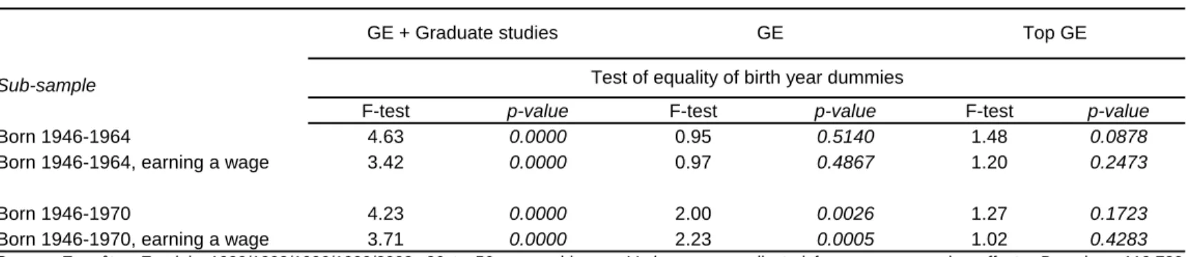
Born 1946-1964 4.63 0.0000 0.95 0.5140 1.48 0.0878
Born 1946-1964, earning a wage 3.42 0.0000 0.97 0.4867 1.20 0.2473
Born 1946-1970 4.23 0.0000 2.00 0.0026 1.27 0.1723
Born 1946-1970, earning a wage 3.71 0.0000 2.23 0.0005 1.02 0.4283
Source: Enquêtes Emploi, 1990/1993/1996/1999/2002; 26 to 56 years old men. Variances are adjusted for survey year-wise effects. Based on 119,720 observations for 1946-1964 (89,126 for wage earners) and 144,958 for 1946-1970 (108,967 for wage earners).
Table 2: Effect of birth year on the proportion of men graduating from elite education
Top GE Test of equality of birth year dummies
coefficient s.e. coefficient s.e. coefficient s.e.
Father Manager/Professional (ref.) - - - - -
-Father Technician/Supervisor -0.1060 0.0049 -0.0258 0.0024 -0.0251 0.0020
Father Self-employed -0.1233 0.0048 -0.0299 0.0023 -0.0300 0.0019
Father Clerical -0.1395 0.0046 -0.0311 0.0023 -0.0316 0.0019
Father Farmer/Manual worker -0.1594 0.0043 -0.0357 0.0022 -0.0359 0.0018
Cohort trend -0.0029 0.0053 -0.0036 0.0028 -0.0033 0.0020
Cohort trend x Father Technician/Supervisor -0.0042 0.0061 -0.0015 0.0032 -0.0004 0.0022
Cohort trend x Father Self-employed -0.0010 0.0059 0.0028 0.0029 0.0028 0.0021
Cohort trend x Father Clerical -0.0017 0.0057 0.0030 0.0029 0.0024 0.0020
Cohort trend x Father Farmer/Man. Worker 0.0006 0.0054 0.0031 0.0028 0.0030 0.0020
Constant 0.1709 0.0043 0.0371 0.0022 0.0373 0.0018
F-test for interacted cohort trends: p-value 0.4409 0.0274 0.0055
Number of observations 115,366 115,366 139,783
Top Grandes écoles : Males born 1946-70
Source: Enquêtes Emploi, 1990/1993/1996/1999/2002; 26 to 56 years old men. Linear probability model. Standard errors are adjusted for survey year-wise effects. The cohort variable is standardized (original mean :1957.78 and s.e.: 7.34).
Table 3: Probability to access elite education, conditional on social origin
Top Grandes écoles : Males born 1946-64 Grandes écoles : Males born 1946-64
coefficient s.e. coefficient s.e. Specification (1)
Non-GE graduate -0.7571 0.0069
Non-GE graduate x cohort trend 0.0259 0.0088 Specification (2)
Non-Top GE graduate -0.8429 0.0155 -0.8247 0.0137
Non-Top GE graduate x cohort trend 0.0483 0.0183 0.0747 0.0146
Cohorte dummies yes yes
Age dummies yes yes
Number of observations 233,189 287,031
Source: Enquêtes Emploi, 1990 to 2002; 26 to 56 years old men. Explained variable is log-wage. Each couple of coefficients is from a separate regression. Standard errors account for the panel autocorrelation structure. The cohort variable is standardized (original mean :1957.78 and s.e.: 7.34).
Table 4: Difference-in-difference wage regression
Males born 1946-1970 Males born 1946-1964
coefficient s.e. coefficient s.e. coefficient s.e. coefficient s.e.
Using GE interactions as instruments
Declared schooling duration 0.0574 0.0004 0.0497 0.0191
F-test for excluded instruments 15.45
Non-GE graduate dummy yes yes
Cohorte dummies yes yes
Age dummies yes yes
Using Top GE interactions as instruments
Declared schooling duration 0.0643 0.0004 0.0584 0.0244 0.0618 0.0004 0.0975 0.0200
F-test for excluded instruments 8.95 13.92
Non-Top GE graduate dummy yes yes yes yes
Cohorte dummies yes yes yes yes
Age dummies yes yes yes yes
Number of observations 230,914 230,914 284,534 284,534
Source: Enquêtes Emploi, 1990 to 2002; 26 to 56 years old men. Explained variable is log-wage. Each coefficients is from a separate regression. Standard errors account for the panel autocorrelation structure. Excluded instruments for schooling time are Non-GE or Non-Top-GE dummy interacted with cohort
Table 5: OLS and IV returns to education
OLS IV
Males born 1946-1964
OLS IV
coefficient s.e. coefficient s.e. coefficient s.e. coefficient s.e.
Using GE interactions as instruments
Declared schooling duration 0.0542 0.0008 0.0858 0.0452
F-test for excluded instruments: 15.45
log minimum wage at entry 0.0773 0.0175 -0.1290 0.1355
F-test for excluded instruments: 1913.58
Non-GE graduate dummy yes yes
Cohorte dummies yes yes
Age dummies yes yes
Using Top GE interactions as instruments
Declared schooling duration 0.0624 0.0008 0.0608 0.0487 0.0564 0.0006 0.0993 0.0401
F-test for excluded instruments: 8.95 13.92
log minimum wage at entry 0.0486 0.0180 -0.0124 0.2327 0.1579 0.0146 -0.0102 0.2150
F-test for excluded instruments: 613.26 96.53
Non-Top GE graduate dummy yes yes yes yes
Cohorte dummies yes yes yes yes
Age dummies yes yes yes yes
Number of observations 230,914 284,534
Source: Enquêtes Emploi, 1990 to 2002; 26 to 56 years old men. Explained variable is log-wage. Minimum wage is expressed in real terms. Standard errors account for the panel autocorrelation structure. Excluded instruments for schooling time and minimum wage are Non-GE or Non-Top-GE dummy interacted with cohort dummies.
Table 6: Impact of minimum wage at labor market entry
IV IV
OLS OLS
coefficient s.e. coefficient s.e.
Using GE interactions as instruments
Declared schooling duration 0.0916 0.0211
F-test for excluded instruments 13.14
Non-GE graduate dummy yes
Cohorte dummies yes
Age dummies yes
Using Top GE interactions as instruments
Declared schooling duration 0.0594 0.0396 0.0953 0.0341
F-test for excluded instruments 4.37 5.01
Non-Top GE graduate dummy yes yes
Cohorte dummies yes yes
Age dummies yes yes
Number of observations 184392 235070
Source: Enquêtes Emploi, 1990 to 2002; 26 to 56 years old men, with more than 10 years of schooling. Explained variable is log-wage. Each coefficients is from a separate regression. Standard errors account for the panel autocorrelation structure. Excluded instruments for schooling time are Non-GE or Non-Top-GE dummy interacted with
Males born 1946-1964 Males born 1946-1970
Table 7: IV returns to education, restricted to individuals with 10 years of schooling or more
Figure 1 Figure 2 0 .0 5 .1 .1 5 .2 1930 1940 1950 1960 1970 1980 c Top GE GE GE + Graduate Stud.
Male schooling shares by cohort
0 .0 5 .1 .1 5 .2 1930 1940 1950 1960 1970 1980 c Top GE GE GE + Graduate Stud.
Figure 3: Cohort specific relative wage - Males born 1946-1964 -.9 -. 85 -. 8 -. 75 -. 7 -. 65 1945 1950 1955 1960 1965 c
cohort gap linear trend
95% conf. int. 95% conf. int.
Control group: GE
-1 .2 -1 -. 8 -. 6 -.4 1945 1950 1955 1960 1965 1970 ccohort gap linear trend
Figure 4