Paleoclimatic variability inferred from the spectral analysis of Greenland and Antarctic ice-core data

HAL Id: hal-03230733

https://hal.archives-ouvertes.fr/hal-03230733

Submitted on 20 May 2021

HAL is a multi-disciplinary open access

archive for the deposit and dissemination of

sci-entific research documents, whether they are

pub-lished or not. The documents may come from

teaching and research institutions in France or

abroad, or from public or private research centers.

L’archive ouverte pluridisciplinaire HAL, est

destinée au dépôt et à la diffusion de documents

scientifiques de niveau recherche, publiés ou non,

émanant des établissements d’enseignement et de

recherche français ou étrangers, des laboratoires

publics ou privés.

Paleoclimatic variability inferred from the spectral

analysis of Greenland and Antarctic ice-core data

P. Yiou, K. Fuhrer, L. Meeker, J. Jouzel, S. Johnsen, P. Mayewski

To cite this version:

P. Yiou, K. Fuhrer, L. Meeker, J. Jouzel, S. Johnsen, et al.. Paleoclimatic variability inferred from the

spectral analysis of Greenland and Antarctic ice-core data. Journal of Geophysical Research. Oceans,

Wiley-Blackwell, 1997, 102 (C12), pp.26441-26454. �10.1029/97JC00158�. �hal-03230733�

JOURNAL OF GEOPHYSICAL RESEARCH, VOL. 102, NO. C12, PAGES 26,441-26,454, NOVEMBER 30, 1997

Paleoclimatic variability inferred from the spectral

analysis of Greenland and Antarctic ice-core data

•,4 j jouzel,1

• L. D Meeker,

.

P. Yiou, 1 K. Fuhrer,

.

S. Johnsen,

•'6 and P. A. Mayewski

•

Abstract. PMeoclimate variations occur at various time scales, between a few

centuries for the Heinrich events and several hundreds of millenia for the glacial

to interglacial variations. The recent ice cores from Greenland (Greenland Ice

Core Project and Greenland

Ice Sheet Project 2) and Antarctica (Vostok) span

at least one glacial oscillation and provide many opportunities to investigate

climate variations with a very fine resolution. The joint study of cores from both

hemispheres

allows us to distinguish between the sources

of variability and helps

to propose mechanisms of variations for the different time scales involved. The

climate proxies we analyze are inferred from •1sO and •D for temperature and

chemical

species

(such as calcium)

for the joint behavior

of the major ions in the

atmosphere, which yield an estimate of the polar circulation index. Those data

provide time series of climatic variables from which we extract the information

on the dynamics of the underlying system. We used several independent spectral

analysis techniques, to reduce the possibility of spurious results. Those methods encompass the multitaper spectral analysis, singular-spectrum analysis, maximum entropy method, principal component analysis, minimum bias spectral estimates, and digital filter reconstructions. Our results show some differences between the two hemispheres in the slow variability associated with the astronomical forcing. Common features found in the three ice-core records occur on shorter periods, between 1 and 7 kyr. The Holocene also shows recurrent common patterns between Greenland and Antarctica. We propose and discuss mechanisms to explain such behavior.

1. Introduction

Deep ice-core data provide a mine of information of

climate variability over a wide range of time scales, ow- ing to their very fine resolution and their time span.

The recent European(Greenland Ice Core Project(GRIP)) and American (Greenland Ice Sheet Project (GISP2)) cores from Greenland and the Vostok core from Antarc- tica are the longest ice cores, to date, and they all span at least one glacial-interglacial cycle. The GRIP

•Laboratoire de Mod61isation du Climat et de l'Environnement,

Commissariat/t l'Energie Atomique, Gif-sur-Yvette, France.

2Physikalisches Institut, Universitat Bern, Bern, Switzerland. 3Department of Mathematics, University of New Hampshire, Durham.

4Also at Glacier Research Group and Climate Change Research Center,

Institute for the Study of Earth, Ocean, and Space, University of New

Hampshire, Durham.

SGeophysical Institute, University of Copenhagen, Copenhagen, Denmark. 6Science Institute, University of Reykjavik, Reykjavik, Iceland.

7Glacier Research Group and Climate Change Research Center, Institute for the Study of Earth, Ocean, and Space, University of New Hampshire,

Durham.

Copyright 1997 by the American Geophysical Union.

Paper number 97JC00158. 0148-0227/97/97JC-00158509.00

ice core [Dansgaard

et al., 1993] was drilled on the

ice divide at Dome Summit (72ø34'N, 37ø37'W) and

30 km west of GRIP [Grootes et al., 1993] and reached

the bedrock at 3053.4 m and penetrated 1.55 m into

bedrock. The accumulation rate averages 20 cm/yr; therefore the cores were expected to give detailed infor-

mation over more than one paleoclimatic cycle, but it is now almost certain that fully reliable time series are

limited to the last 110 kyr B.P., the older

part being

dis-

turbed due to the proximity of the bedrock [Bender et al., 1994; Chappellaz et al., this issue]. The annual cycle

can be visually detected on the top parts of the cores, which has therefore an absolute chronology. Annual layer counting was performed on the GISP2 ice core down to •0 50 kyr B.P., and the chronology was then es-

tablished

through

correlations

with the •sO of oxygen

in

air bubbles between Greenland and other records were performed by Bender et al. [1994]; the GISP2 time se-

ries in this study use this chronology. The new GISP2 annual layer chronology now extends to 110 kyr B.P.

[Meese et al., this issue]. The top 14.5 kyr of the GRIP

ice core were also dated by annual layer counting, and

the rest of the core was dated with the use of glacio-

logical models [Dansgaard et al., 1993; Johnsen et al.,

26,442 YIOU ET AL.: PALEOVARIABILITY FROM ICE-CORE DATA

1995] . The Vostok project is a cooperative effort be- tween Russia, the United States, and France [Vostok

Project Members, 1995]; it was drilled in East Antarc- tica (78ø28•S, 106•48•E) and is presently 3125 m deep.

The accumulation rate is about 2 cm/yr; this means that the annual layers are too thin for visual detection and models of chronologies have to be used to date the samples [Lorius e! al., 1985; Jouzel e! al., 1993; Wael-

bvoeck et al., 1995].

From these ice cores, climatic information was re-

trieved through isotopic measurements of oxygen 18

[Dansgaard et al., 1993; Grootes et al., 1993] and deu- terium [Jouzel et al., 1993], greenhouse gases (CO2 [Barnola e! al., 1987] and CH4 [Chappellaz et al., 1990, 1993]), dust content [Petit et al., 1990], electrical con- ductivity [Taylor et al., 1993] and various chemical species [Legrand et al., 1992, 1993; Mayewski e! al.,

1993a, 1993b, 1994, this issue]. We focused on the iso-

topic

measurements

((•1sO

and 5D), expressed

in perrail

with respect to the standard mean ocean water, and chemical species in the Greenland records. The two isotopes mainly account for the local temperature vari- ations at the top of the inversion layer, where the pre-

cipitation formed [Jouzel and Merlivat, 1984; Johnsen

et al., 1989; Jouzel et al., this issue], while the chemical species are proxies for the intensity of the polar circu-

lation [Mayewski et al., 1993a].

The time series derived from the experimental mea- surements are generally irregular but bear many re- semblances and recurring patterns embedded in noise. These patterns cover the well-documented glacial-inter- glacial cycle and the abrupt oscillations during the last ice age that are found in all cores. Our challenge is then to decipher the climatic information from these appar- ently noisy signals and assess the statistical significance of the near periodicities in order to infer plausible phys- ical mechanisms.

Our strategy is to cut our records into identifiable

climatic periods. The main reason is that climate dy-

namics is not necessarily stationary on all time scales.

For example, if we look at climatic variations occurring on time scales of centuries to millenia either during an ice age or during an interglacial interval, the two in-

tervals (cold and warm) have very distinct regimes and

a global analysis would only average those differences without an appropriate investigation of the proper dy- namics of each regime. On the other hand, if we look at

slower variations linked to orbital forcing [Hays et al., 1976; Berger et al., 1993], then we obviously need to

consider the full length records and the minute temporal details are no longer necessary. Therefore we adapted the time "windows" from the paleoclimatic signals to the processes at play on each characteristic time scale. This methodology is a time-frequency analysis where we have introduced our a priori knowledge of the cli-

matic system.

Massive iceberg discharges from the Laurentide and the Scandinavian Ice Sheets during the last ice age have

been documented recently [Heinrich, 1988; Bond and Lotti, 1995] and generically called "Heinrich events"

[Broecker eta!., 1992]. They have been associated with

sea surface temperature variations over the North At-

lantic and temperature variations over Greenland [Bond et al., 1993; Pat!lard and Labeyrie, 1994]. This cumula- tive evidence points to global climate instability during the last glacial age. This is why we elected to study

this particular period of climate history, with its high

variability.

The Holocene (11.6 kyr B.P. to present) is the in-

terglacial period we are presently enjoying. Its last 10 kyr have proved to be remarkably stable, compared

to glacial-to-interglacial variations [Johnsen et al., 1992].

Fluctuations in the Holocene glaciochemical series, al- though small compared to those in the glacial portion of

the record, reveal marked variability in climate [ O'Brien et al., 1996]. Nevertheless, these little variations testify

to internal climate variability involving the atmosphere and the ocean during a globally stationary climate and

possible (but unknown) solar or volcanic forcings [Stu-

iver et al., 1995]. Hence we picked this period, in addi- tion to obvious reasons that concern human civilization.

In this paper, we summarize methodological guide- lines for time series processing; we particularly insist

on the necessity of robust and stable methods, due to

the many irregularities in most paleoclimatic signals. These techniques include singular spectrum analysis, the multitaper method, the maximum entropy method, minimum bias spectral estimates, and digital filter re- constructions. Then we apply these recent techniques to the ice-core data described in section 3, for the three cli-

matic periods we described above. The results are given

in section 4, where we also propose physical mechanisms to interpret them.

2. Methods

In this section, we describe a few new numerical tech-

niques to extract information from time series. It is

important to note that climatological time series very

seldom verify the hypotheses required by any mathe- matical method and that several techniques should be

used as cross checks for the validity and stability of re- sults [Ghil and Yiou, 1996; Yiou e! al., 1995]. Most

of the methods here are implemented in a public do-

main computer tool kit (SSAToolkit) developed by Der- linger et al. [1994] (available on the world wide web at http://www.atmos.ucla.edu/). In companion papers

[Mayewski

et al., this issue;

Meeker

et al., this issue],

al-

ternate techniques, but based on similar principles, are used to extract periodic components. We briefly discuss them in the Appendix.

2.1. Sampling

Data sampling (or resampling) is an important step

prior to time series analysis, in the field of paleodata processing. Most signal analysis methods require a reg-

YIOU ET AL.: PALEOVARIABILITY FROM ICE-CORE DATA 26,443

ular time sampling, which is generally not the case for ice-core data. An array of interpolating techniques is described and tested by Benois! [1986] and Yiou et al.

[1995]. It has been shown that the interpolation method

of choice can affect the spectral estimates in the high fre- quencies, hence limiting the relative confidence in this

part of the spectrum [Yiou et al., 1995]; overall, how-

ever, less than one third of the frequency range seemed affected by the choice of the interpolating method.

The technique we adopted proceeds by averaging the signal over nonoverlapping "bins" of equal time inter-

vals •- [Benoist, 1986; Yiou et al., 1995]. This scheme corresponds to a weak low-pass filter [Benoist, 1986].

The property of this interpolation process is that the Nyquist p•-;• ;o or. tr the in•nnslc process does ,,v•

contain power in the [-l/r, l/r] frequency band, then

the aliasing is negligible with this interpolating scheme.

Numerical experiments [Yiou et al., 1995] show that it does not create spurious oscillations (contrary to regu-

lar cubic spline methods) and hence the spectrum can

be estimated with more confidence. On the other hand,

this method is only useful when one is willing to under-

sample the time series, i.e., if r is greater than a typical

time step of the signal. If oversampling is desired, an- other type of interpolation, using the physical relation linking depth and time in order to preserve the data skewness, can be used, with little spectral alterations. 2.2. Singular Spectrum Analysis

Singular spectrum analysis (SSA) is designed to ex-

tract information from short and noisy time series and

give hints on the (unknown) dynamics of the underly-

ing system that generated the series [Broomhead and

King, 1986; Vautavd and Ghil, 1989]. It was moti- vated by mathematical and experimental results [Tak-

ens, 1981; Packard et al., 1980], which showed that under generic conditions, a time series of observables from a dynamical system contains enough information to reconstruct this "unknown" dynamical system. The starting point of the method is to embed a time series

{X(t)}, t = 1,...,N in a vector space of dimension

M, with M presumably larger than the effective but unknown dimension d of the underlying system. The

embedding procedure constructs a sequence {X(t)} of

M-dimensional vectors of delayed coordinates from the time series X:

.•(t) = [X(t),X(t + 1),...,X(t + M- 1)], (1)

with t = 1,..., N- M + 1. If d is larger than four or the

time series contains (random) noise, a raw application

of this technique will fill any two-dimensional projection in a dense way so that no information can be retrieved. SSA allows us to unravel the information entangled in the delayed coordinate phase space by decomposing the constructed sequence of vectors into elementary oscil- lation patterns. Hence this method generates data- adaptative filters for the separation of the time series into statistically independent components, like trend,

deterministic oscillations, and noise. Thus a clean sig- nal can be analyzed through reconstructed components

(RCs), pattern-wise

or by using other mathematical

tools [Allen, 1992; Vautard ½! al., 1992]. Details of SSA algorithms and properties have been investigated

by Penland et al. [1991], Vautard et al. [1992], and

Allen [1992].

An important step in signal processing (and SSA in

particular)

is the quantitative

detection

of noise

and its

characteristics. Climatic time series are often contam- inated by red noise, which affects preferably low fre-

quencies; it is a first order autoregressive process whose

spectral

characteristics

(• 1If 2 shape

in a frequency

diagram) are generic

in climate time series

[Ghil and

cruoe r•'• .... no,. •hen, I•]. In general, very ---•-

tests can be devised from comparisons with an "ideal-

ized" noise process: the spectrum of a noise process is

known to have a particular shape, and if the data spec- trum lies above an ideal noise spectrum, it is generally considered as "significant." This approach can be very deceptive because a single noise realization can have a very different spectrum from an ideal one, especially if the number of data points is small; it is the average of such spectra over many realizations that will tend to

the spectrum of the ideal noise process. Allen [1992] devised tests to compare the statistics of simulated (or surrogate) red noise time series with those of a climatic signal; this is the Monte Carlo SSA (MC-SSA). Alter-

natives to MC-SSA, based on a standard procedure of

principal component analysis [Preisendorfer, 1988] to

estimate distributions of serial correlations, can also be

used with a smaller computing cost [Lall and Mann, 1995]. Multivariate generalizations of (MC-) SSA have been developed by Plaut and Vautard [1994] and Allen and Robertson [1996].

2.3. Mul•i•aper Method

The purpose of this nonparametric spectral method

[Thomson,

1982; Percival and Walden,

1993] is to cir-

cumvent the problem of the variance of spectral esti- mates; indeed, the variance of raw Fourier spectrum

of a random process equals the spectrum itself [Jenkins and Watts, 1968], which means that the potential errors can be as large as the calculation itself. A set of inde-

pendent estimates of the power spectrum is computed, by premultiplying the data by K orthogonal tapers, i.e.,

functions which are built to minimize the spectral leak-

age outside a scaled bandwidth N9 (9 is a frequency

bandwidth)

due to the finitehess

(N) of the data. Then,

averaging over this ensemble of spectra yields a better

and more stable (with lower variance)

estimate than

with single-taper

methods

[Thomson,

1990]. Detailed

algorithms for the calculation of those tapers are given

by in Thomson

[1990],

Percival

and Walden

[1993],

and

RSgnvaldsson [1993]. The choice of K and N• is a

trade-off between stability and frequency resolution, so

26,444 YIOU ET AL.: PALEOVARIABILITY FROM ICE-CORE DATA

Harmonic

analysis

(estimate

of line frequencies

and

their amplitude)

can be performed

by MTM, with a

statistical F test on the amplitude. One of the main

assumptions

of MTM harmonic

analysis

is that the sig-

nal must yield periodic

and separated

components.

If

not, a continuous

spectrum

(from a colored

noise

or a

chaotic

system)

will be broken

down to spurious

lines

with arbitrary frequencies

and possibly

high F values.

This is a danger

of the method,

which

can be partially

avoided if the raw power spectrum is computed, hints

for lines are detected,

and the parameters

Nft and K

are varied.

Time-frequency analyses (evolutive spectral analyses)

with moving windows were performed with this method

by Yiou et al. [1991] and Birchfield and Ghil [19931. In addition, a multichannel MTM generalization (i.e., with a spatial extent) has been investigated by Mann et al. [1995].

2.4. Maximum Entropy Method

The maximum entropy method (MEM) is potent to

estimate line frequencies in an autoregressive time se-

ries. Exhaustive details are given by Burg [1967] or Childers [1978].

MEM is very efficient for detecting frequency lines

for stationary time series. If this hypothesis is not ver- ified, or if the time series is not close to autoregressive,

cross testing the time series with other techniques is necessary. Moreover, the behavior of the spectral es- timate depends on the choice of the autoregression or- der M: the number of peaks in the spectrum increases with M, regardless of the time series content. An upper

bound for M is generally taken as N/2. Heuristic crite- ria have been devised to refine the choice of a reasonable M [Haykin and Kessler, 1983; Benoist, 1986], based on

a minimization of the residual of a least squares fit be-

tween the autoregressive approximation and the origi-

nal time series [Haykin and Kessler, 1983]. The rise of

such criteria can be tricky because they all appear to

underestimate the order of regression of a time series

[Benoist, 1986]. Thus they still do require trial-and- error sensitivity tests [Yiou e! al., 1996].

2.5. Empirical Orthogonal Function Analysis

Empirical orthogonal function (EOF) analysis [P½izoto and Oort, 1992], like principal component analysis (PCA) [Peisendorfer, 1988], is used for multivariate data in the

hope that a new basis can be found so that the infor- mation in the data is expressed with fewer coordinates. Its formulation is quite similar to the SSA method and it is useful for data with more than two variables. In principle, SSA theory can be embedded into PCA, as the computations essentially involve the diagonalization of a covariance matrix and projections onto the eigen- vectors. We exposed at length SSA in this paper, thus we will be very brief for PCA, which is used to extract a common variation component within a set of chemical measurements.

In practice, we have a sequence of vectors V•, n = 1,...,N, e.g., eight-dimensional vectors representing the variations of chemical species measured in the GISP2

ice core [Mayewski

et al., 1994]. Then we want to

compute a basis in this multi dimensional space (eight- dimensional in this particular case), in which the vari-

ance is most efficiently represented; that is, it can be

described by the least possible number of vectors. If V denotes the N x M matrix containing the sequence of

N data M-dimensional vectors V,, then the covariance

C of the matrix V is 1

(2)

where the superscript t denotes matrix transposition.

We then look for the eigenelements of the symmetric and definite positive matrix R by solving

Re• = ,k•e•, (3)

where the M vectors e• are called the EOFs, as with

SSA. Projections P• of the data V onto this eigenbasis can be defined as

r• - e• V.

(4)

They give a new representation of the data in which

each P• represents ,k•/,X• +... + ,k•u percent of the co- variance of V.

For example, the first and the second EOF in the GISP2 chemical species record represent 70% and 14%, respectively, of the variance of the data.

3. Data

As explained in the introduction, we focused on two

types of data with a very high temporal resolution: iso- topes and chemical species. The GISP2 chronology we use is based on annual layer counting down to • 50 kyr

and then derived

by correlations

with •sO of O•. [Bender

et al., 1994]. For the GRIP ice core, the chronology was

based on layer counting down to 40 kyr; the rest of the

core was dated with a glaciological model [Dansgaard e! al., 1993] and correlation with a marine-sediment record [Grootes et al., 1993].

The Vostok records were dated using a glaciologi-

cal model [Jouzel et al., 1993] with a control point

at 110 kyr B.P., where the record is assumed to be synchronous with the Spectral and Mapping Project

(SPECMAP) record at marine stage 5 [Jouzel et al., 1993]. Alternative chronologies based on correlation with deep-sea core records [Sowers et al., 1993] or or- bital tuning [Waelbroeck et al., 1995] have also been

explored. 3.1. Isotopes

We studied oxygen 18 (GRIP/GISP2) and deuterium (Vostok) from the core water. Those values are nor- realized to standard mean ocean water (SMOW) and

expressed in per mil delta values. These isotopes are proxies for the temperature of formation of the precip-

YIOU ET AL.: PALEOVARIABILITY FROM ICE-CORE DATA 26,445 itation (at the inversion layer) as shown by numerical

[Jouzel

and Merlivat, 1984; Jouzel

et al., 1994] and ex-

perimental studies [Johnsen et al., 1989]. Jouzel et al. [this issue] review the assessment of the temperature-

isotope relationship. The relationship between the iso- topic content of snow and temperature at the precipi-

tation site has been investigated for Greenland through

observations of present-day distribution in surface snow

[Johnsen et al., 1989] and examined through a hierarchy of isotopic models [Jouzel et al., this issue and references therein]. The use of present-day spatial temperature-

isotope gradient for interpreting the Greenland isotopic profiles has been challenged by recent paleothermome-

try measurements [Cuffey et al., 1995; Johnsen e! al.,

1995b]. Those two studies led to the conclusion that the isotopic ratios can be used as palcothermometers, and each group has, using different calibration procedures, produced a central Greenland temperature record. We have based our spectral analyses on the isotopic records themselves and checked that the spectral properties are not significantly modified when the temperature records inferred either from the present-day isotope relationship

(throughout the records as currently done at Vostok) or

time dependent calibration [Cuffey et al., 1995; Johnsen et al., 1995b] are used.

The sampling for all the cores is continuous and de- tailed: 55 cm, i m at GISP2, and either 50 cm or 1 m

at Vostok (with few 2-m samples). Therefore the time sampling varies from a few years (the upper part of the Greenland cores) to 100 years, with larger sam-

pling intervals

(up to 200 years) for the periods

near

50, 60, and 100 kyr B.P. at GRIP, GISP2, and Vostok, respectively. Therefore we generated several time series

with different time steps (and the interpolating tech-

nique described above) from each record, depending on

the length of the records (full record, glacial period, or

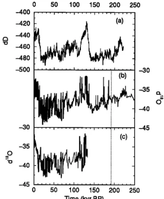
Holocene) and the time scale to be investigated. The full-extent isotopic profiles for the three cores are shown in Figure 1.

3.2. Soluble Ions

Soluble ions (Ca, Na, C1, SO4, K, Mg, NH4, and NOs) were measured at a resolution of 0.6-2.5 years

through the Holocene, a mean of 3.48 years through the deglaciation, m 3-116 years throughout the remainder of the 110,000-year long portion of the record, and at lower resolution over the rest of the core, for a total of

16,395 samples [Mayewski et al., 1990b, 1993a, 1993b, 1994, this issue; Fuhrer et al., 1993]. The sources for the chemical species transported to Greenland are primar- ily terrestrial dust and marine surfaces [Mayewski et al., 1990a]. It was suggested that changes in atmospheric composition could be accounted for by changes in the size of the polar atmospheric cell, resultant changes

in source regions and the modifications of continental

biogenic source regions [Mayewski et al., 1993a, 1993b,

1994]. Similarly,

Alley et al. [1996]

used

a simple

model

to show

that the chemical

concentrations

(in the GISP2

0 50 100 150 200 250

-420

(a)

-40

Figure Z. Isotopic

variations

in the (a) Vostok,

(b)

GRIP and (c) GISP2 ice cores. The profiles are ex- pressed in per mil versus SMOW; time goes from the

right to the left and is expressed

in kiloyears

B.P. Fig-

ure la shows deuterium content, and Figures lb and lc

show oxygen 18 content. The vertical dotted bar in the Greenland ice-core profiles indicates the time restriction

we took (110 kyr B.P.) for our spectral analyses.

snow and ice) follow atmospheric fluxes and hence pro-

vide a history of atmospheric

circulation

[Mayewski

et

al., this issue].

The GISP2 ion measurements were grouped by a principal component analysis, as described previously

in order to highlight their similitudes and differences.

This allowed us to create robust composite variables of

the climate system,

by identifying

strong

and recurrent

patterns of oscillations. The average time sampling is

very fine, but we subsampled the data to a time inter-

val of r - 200 years to make comparisons with isotopic

data possible.

The ion concentrations

are all positive

with a strong

asymmetry toward large values. Hence we normalized

them through their logarithm in order to preserve sta- tionarity and symmetry between lower and higher val- ues. Indeed, noise tests generally assume that the pro-

cesses are at least pseudo-Gaussian, which would not be

the case if the raw data were used. Spurious harmonics can also be introduced if a Fourier analysis is performed. It turns out that our results are only marginally affected

when replacing the raw unnormalized data.

We plotted the temporal variations during the last ice

age of Ca (GRIP [Fuhrer

et al., 1993])

on a logarithmic

26,446 YIOU ET AL.. PALEOVARIABILITY FROM ICE-CORE DATA -34 -36 -38 -40 -42 -44 -0.04 •' -0.02 to 0.00 0.02 0 LU 0.04 -2 0 o 1 2 • 3 0 20 40 60 80 100 120 Time (kyr BP)

Figure 2. (a) For comparison

purposes

the $1aO

pro-

file at GRIP during the last ice age is plotted. (b) The

log-transformed calcium variations during the last ice

age at GRIP. (c) The EOF1 variations of eight chem-

ical species measured at GISP2 are shown. Time axis

and units are as in Figure 1.

(in fact, anticorrelated)

to the (•180 values

at GRIP

(Figure 2a), with a high correlation coefficient, r 2 =

0.79; the linear regression relation

J•SO

- -38.42 - 1.38

log(Ca),

(5)

exhibits fairly low dispersion (Figure 3a). This means that calcium values are high during interstadials (cold

periods,

with low 5•sO). Surprisingly,

it turns out that

this dispersion is close to the one in 51sO-temperature

relations. We notice that the calcium-oxygen 18 rela- tionship during the last glacial period is divided into two clusters with different slopes. This suggests the existence of two dynamical atmospheric regimes in the glacial climate, during stadials and interstadials; they are linked to the nonlinear saturation of climate insta- bilities on this time scale [Ghil et al., 1991].

To first order, 5•SO and chemical

species

seem

to be

driven in the same way by local (northern high latitude)

climate

changes.

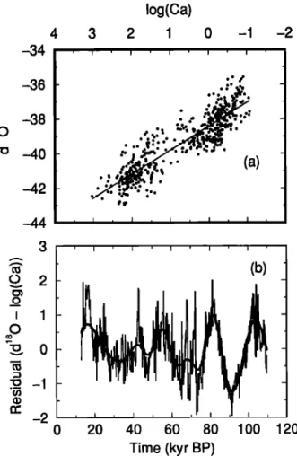
The residual

rc- 5•SO-a log(Ca)-b,

with a - -1.38 and b - -38.42, would then account for processes that are not governed by local temperature, like processes occurring or driven at low latitudes. The variations of rc are plotted in Figure 3b.

On the other hand, the first EOF of the chemical

species assemblage from the GISP2 ice core [Mayewski et al., 1994], plotted in Figure 2c, has a much smaller

correlation coefficient with the (•180 record at GISP2 or

GRIP (r 2 = 0.25, not shown):

there

seems

to be a first-

order linear relationship comparable with that of Ca at GRIP, but the dispersion is much higher. Therefore we did not create a composite residual variable from this EOF and an isotopic record.

4. Results

We focused on three characteristic time scales rele-

vant to paleoclimate variations. This circumvents the possibility of nonstationarity of the records (and the

system

itself) because

it is very likely that the climate

system wanders through different states (even during an ice age) for which only local stationarity can be as-

sumed

limbtie e! al., 1992].

4.1. Glacial-Interglacial Oscillation

The study of the full-extent records was done to cir-

cumscribe the role of the astronomical forcing on long

time scales. This role has already been documented

extensively,

in marine

cores

(Crowley

and North [1991]

give many examples)

and in ice cores

[Benoist,

1986;

log(Ca) 4 3 2 1 0 -1 -2 -34 -36

•0 -38

•o -40

• 3

,,

•'

1

0

n' -2

Figure 3. (a) The linear regression

between

(•180 and

log(Ca). (b) Plot of the residual

rc, expressed

in J•sO

per mil, from the linear regression from Figure 2c (thin line). The thick line is the reconstruction of SSA prin-

cipal components i and 2, which account for the slowly

YIOU ET AL.' PALEOVARIABILITY FROM ICE-CORE DATA 26,447

Jouzel et al., 1987; Johnsen et al., 1995a; Waelbroeck

e! al., 1995], with various techniques. We concen-

trated on isotopic

records

from the Vostok (5D) and

the two Greenland

cores

(Slso), which span a com-

plete glacial-interglacial cycle and include an excel-

lent resolution for the Holocene. We sampled the data

with an average step of v = 0.5 kyr. MTM analy- ses show that low-frequency components close to the

Milankovitch frequencies (obliquity, 41 kyr; precession of equinoxes, 23 kyr and 19 kyr) are present in all

records. The very low frequency component, associ-

ated with the full glacial-interglacial oscillation, can hardly be interpreted based on eccentrity forcing, be-

cause it is observed at most twice in the Vostok record

and only once in the Greenland cores. An obliquity

component (around 41 kyr) appears in Figure 4 in the Vostok ice core (dated from the extended glaciological timescale [Jouzel et al., 1993]) and in the Greenland records (in Figure 5, and shown by Mayewski e! al. [this issue]). This component is more stable in the Vostok isotopic signal than in the Greenland signals, possibly

due to the different lengths of the records or the differ-

ent chronologies. On the other hand, precessional com-

ponents

(around

23 kyr) appear

to be more stable and

with a larger relative amplitude

(with respect

to MTM

parameter changes) in the Greenland records than in the Vostok one.

An important caveat of this analysis is that it cannot

be confirmed

by MEM because

it requires

very large

autoregressive

orders (which are several

times larger

than the one preconized

by standard

tests

[Haykin

and

Kessler,

1983]) in order to find Milankovitch

frequen-

cies. MC-SSA is not sensitive enough to assess the pres- ence (or absence) of such slow variability.

The slight discrepancy

between

the two hemispheres

can have essentially two origins. The first is rather

technical

and would be errors in the chronologies

of

one or all the records. The chronologies are trusted to

have 10% error bars in age, but local perturbations of

such

amplitude

can induce

changes

in the low-frequency

15 , ... 1.00 • 10 0.95 E --,. • 5 0.90 • 0 , 0.85 100 10 Period (kyr)

Figure 4. MTM harmonic analysis of the Vostok deu-

terium record. The parameter values are NO -- 2 and

K - 3 tapers. The horizontal

axis represents

period

(in

kiloyears),

the left axis is estimated

amplitude

(light

solid line) and the right axis is the statistical F test

(heavy

solid line).

1.5 1.o 0.5 o.o lOO Period (kyr) 10 1.00 0.95 0.90 0.85

Figure 5. MTM harmonic analysis of the GRIP oxy- gen 18 record. The MTM parameters and axis captions are the same as in Figure 4.

spectra. Experiments with different chronologies for the

Vostok deuterium record have been performed [Wael- broeck et al., 1995] but they were based on orbital tun- ing [Martinson et al., 1987] of the chronology, for which

the identification of Milankovitch frequencies can be bi- ased because they are deliberately introduced into the

signal. On the other hand, if the chronologies are (pro- visionally) trusted not to alter the spectra in the low-

frequency

band (and this is a bold assumption),

then

climatological explanations can be attempted: the pre- cessional forcing affects most strongly the Asian mon-

soon [Kutzbach and Otto-Bliesner, 1982; Kutzbach and Guetter, 1984]. This is coupled to the Arctic, but not

to the Antarctic circumpolar circulation, via the flow

over Tibet and Siberia [Marcus et al., 1994, 1996]. An alternate explanation is that the Antarctic circumpolar

vortex reduces the influence of the meridional transport

from the low latitudes to Antarctica, hence altering its

precessional component which is mostly found in equa-

torial and tropical latitudes [Crowley and North, 1991; Imbrie et al., 1992].

4.2. Glacial Period

We took the deuterium profile at Vostok and the oxy-

gen 18 and (previously defined) Ca residual records in

GRIP/GISP2 to study the glacial

period (110 to 13 kyr

B.P.). The records were sampled every 200 years. The

general shape of the MTM and MEM spectra is akin

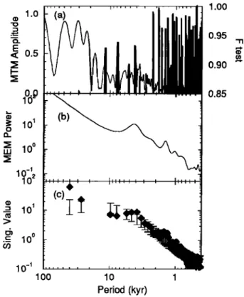
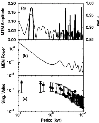
to that of red noise, with a few frequency bumps (Fig- ure 6).

From a MC-SSA analysis, the Vostok record con- tains components with periodicities near 37 and 18 kyr which can be attributed to obliquity and precessional

changes (Figure 6c). These periodicities are also de- tected by MTM (Figure 6a), but not with MEM, using

a moderate

autoregression

order (M = 20, Figure 6b).

The higher frequencies contain significant components

around 10 and 6 kyr. The former could be a precessional

harmonic

[Yiou e! al., 1991; Hagelberg

et al., 1994],

but

the 6 kyr near cycle is close to the behavior predicted by simple ice sheet oscillation models [Ghil and Le Treut,

1981; MacAyeal, 1993]. From these results only, we

26,448 YIOU ET AL.: PALEOVARIABILITY FROM ICE-CORE DATA o

Q- 02

._.c O•

0.95 "n

Figure 6. Spectral analyses of the glacial Vostok deu-

terium record. (a) A MTM harmonic analysis (Nf• = 4 and K = 7); left and right axis as in Figures 4 and

5. The logarithmic horizontal axis is period, expressed

in kiloyears. (b) A MEM spectrum

(M = 20). (c)

A Monte Carlo SSA analysis, with a window width of

M = 60. The error bars give the 90% red noise per-

centiles: the diamonds falling between the bars cor- respond to signal components which are 90% indistin- guishable from red noise.

hemisphere ice sheets) is susceptible to provoking such

oscillations, but evidences of iceberg discharges around

West Antarctica [Shemesh et al., 1994] could give such

an explanation. A reconstruction associated with this component reveals variations close in amplitude to the

largest fluctuations observed in the raw data during the

glacial period, as already shown by Yiou et al. [1994].

The rest of the spectrum is either statistically in-

distinguishable from red noise or has very low ampli- tude peaks that cannot be interpreted in simple phys- ical terms. We performed similar analyses on time se- ries based on a chronology obtained with correlation

with SPECMAP data through dlSO in 02 [Sowers

et

al., 1993]. This correlation, which roughly corresponds

to a compression of the chronology during the last ice age, reduces to •-, 4 kyr the periodicity of the oscillation we detected in Figure 6 with the timescale of Jouzel e!

al. [1993]. This result (not shown) is not very surpris-

ing, and it allows us to give an interval for the average

periodicity of this oscillation.

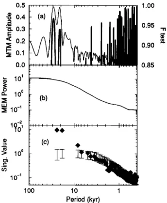
The Greenland (•180 records have a similar behav-

ior in the low-frequency band, as noticed by Yiou e!

al. [1995]. The ion concentration records yield the

same spectra (not shown) as the isotopic record, and

the behavior of the EOF1 at GISP2 was investigated

by Mayewski et al. [1993, 1994] who found similar re-

sults. But the records seem to contain slightly faster millenial components, with periods between 4 and 5 kyr

(Figure 7). This type of behavior has already been as-

sociated with the massive iceberg discharges from the

Laurentide Ice Sheet into the North Atlantic [Bond e! al., 1993; Yiou et al., 1994]. These discharges are not exactly periodic (in a strict mathematical sense), and

other Northern Hemisphere ice sheets can discharge ice-

bergs too [Bond and Lotti, 1995]; therefore it is antic-

ipated that what is observed through spectral analysis is an average periodicity of such a phenomenon. Yet, the timing of Heinrich events can be approximated by an • 6-kyr band-pass component in the glaciochemical

time series

[Mayewski

et al., this issue].

A comparable resolution in both cores allows us to

investigate the connection between the almost cyclical features in the Greenland and Antarctic cores. Bender

e! al. [1994] have put the GISP2 and the Vostok isotopic

records

on a common

timescale,

through

dlSO content

in air bubbles, and found that each interstadial in Vos- tok coincides with a long intersradial in GISP2. Such a synchroneity on this time scale would imply a global oscillating mechanism whose response time involves at least one ice sheet instability; the Laurentide ice sheet is then a good candidate to drive such variability. Bender

et al. [1994] argue that the connection to the south-

ern hemisphere can go through the thermohaline cir-

1.0 0.5 , 1.00 0.95 0.90

10dP

0.85

•:

0 o

(c)It

=e 1ø

c

• 100

Figure 7. Spectral analyses of the glacial GRIP oxy-

gen 18 record

(the GISP2 record

gives

identical

results).

Same

panels

and parameters

as in Figure 6.

YIOU ET AL.' PALEOVARIABILITY FROM ICE-CORE DATA 26,449

culation, as modeled by Ghil et al. [1987]. Indeed,

modifications in the rate at which North Atlantic Deep

Water (NADW) sinks and flows southward has impli-

cations on the southern hemisphere heat budget and

hence temperature. On the other hand, with the "com-

mon" time frame of Bender et al. [1994], the Vostok

record sometimes leads the GISP2 record by i or 2 kyr, and the Greenland ice cores yield a larger number in- terstadials. We propose to reconcile this slight discrep- ancy with possible instabilities of the West Antarctic Ice Sheet and the occurrence of iceberg discharges into the

Southern Ocean: such events, described by Shemesh et

al. [1994], could in turn affect the northern hemisphere

through the ocean circulation or ocean level. A the- ory for such a global ice sheet instability scenario, with several ice sheet oscillators, has also been proposed by

Yiou et al. [1995] and Verbiisky and Salizman [1994, 1995].

In the very high frequency domain, we also note the presence of a significant, almost periodic compo- nent around 1.5 kyr, which was also found in high-

resolution North Atlantic marine records [Stocker and Mysak, 1992; Uortijo et al., 1995]. It is even stronger

in EOF1 of the GISP2 chemical species. This compo-

nent could be attributed to the variability of the oceanic

thermohaline circulation [Weaver et al., 1993; Quon and

Ghil, 1995]. Long-term simulations of coupled ocean-

atmosphere models should assess this component. The chemical species residue rc at GRIP shows a

prominent precessional component (Figures 8a,c) sim-

0.5 0.3 0.2 0.1 0.0

• 101

o 0o

III 0-1

(• 0 o

(b)

•

(c)

.

0.95 -n

Figure 8. Spectral analyses of the glacial GRIP oxy- gen 18 residual rc record. Same panels and parameters

as in Figure 6. 3 o lOO lO (c) 1.00 0.95 0.90 0.85 i

101

10

0

10

-1

Figure 9. Spectral analyses of the last 10 kyr of the

Holocene deuterium record at Vostok. Panels are the

same as in Figures 6-8; the parameters are Nfl = 6 and K = 8 in Figure 9a, M = 20 in Figure 9b and M = 40

in Figure 9c.

ilar to that found in the GISP2 ammonium series de-

rived from mid-low latitude continental biogenic sources

[Meeker et al., this issue]. We reconstructed

this pre-

cessional component with the SSA algorithm [Vautard

et al., 1992], with the first two EOFs, and plotted this

reconstruction in Figure 3. Apart from a periodicity at

9.8 kyr (close

to a harmonic

of a precessional

cycle),

the faster variations are within the red noise statistics

(Figure 8). In particular, no fast variations related to Heinrich events are detected in this "residual" record. This precessional component shows that the nonlocal

climate

variability

(i.e., over source

regions)

of 5180

comes from low latitudes which show larger precessional

components [Crowley and North, 1991]. Therefore it

seems possible to retrieve low-latitude climatic infor- mation from a heterogeneous couple of time series at the same location.

4.3. Holocene

The Holocene period (11.6 kyr B.P. to present) was analyzed on the isotopic series from the Vostok (Fig- ure 9) and GRIP (Figure 10) records. The time sam- pling was taken as r- 50 years. MTM spectra and a noise test with Monte Carlo SSA (Figures 9c and 10c)

show that most of the records are indistinguishable from red noise over most of the frequency range from 1/100 to

1/10000 years-

1. In the GRIP record,

a few fast com-

26,450 YIOU ET AL.' PALEOVARIABILITY FROM ICE-CORE DATA 0.20 = 0.15 E 0.10 i- 0.05 0.00 -- 0 o e 1 o :• 10 -• 10 -2 10 -2 104 100 10 -• 1.00 0.95 0.90 0.85 Period (kyr)

Figure 10. Spectral analyses of the Holocene GRIP oxygen 18 record. Same panels and parameters as in Figure 9.

noise background (Figure 10c) at periodicities around

2 kyr, 180 years, 150 years and 120 years. These pe- riodicities are also found by MTM harmonic analysis

and MEM (Figures 10a and 10b). They are robust to

parameter changes; hence this stability between inde- pendent techniques strongly enhances the confidence of these peaks. The Holocene period in the deuterium pro-

file at Vostok shows similarities with the GRIP record,

with significant components detected by MC-SSA near 180 and 130 years standing out above the red noise spec-

trum. We notice that both MTM and MEM can give

spurious peaks when compared with MC-SSA. This is

due to the fact that both of the former methods tend

to break broadband noise into discrete lines (MTM) or sharp peaks (MEM).

The significant oscillations occur during a relatively ice sheet free period (the Holocene), hence they are less

likely to be associated with glacial events or major ice

sheet (recurring) oscillations. External (e.g., astronom- ical or solar) forcings can play a role on these time scales [Stuiver et al., 1995], even though the physical

mechanisms, the energy variations are very small, re- lating solar constant fluctuations to such climate varia- tions are not yet documented. On the other hand, this type of centennial-to-millenial oscillations starts to be

documented in other high-resolution data [$tocker and

Mysak, 1992; Mann et al., 1995] and models of the gen-

eral circulation of the ocean, either uncoupled [Weaver

and Hughes, 1994; Chen and Ghil, 1995] or coupled with

a sea ice [Yang and Neelin, 1993] or an atmospheric

[Delworlh

el al., 1993; Uhen and Ghil, 1996] model,

are

simulating such oscillations that seem to arise from in- stabilities of the thermohaline circulation.

5. Conclusions

In this paper we have applied advanced techniques

for time series analysis encompassing singular spec- trum analysis, multitaper method and maximum en- tropy method. These techniques allowed us to disen- tangle, to some extent, the complex paleoclimatic infor- mation contained in Greenland and Antarctic ice-core signals through oscillation detection. We have high- lighted the presence of slow components close to the orbital frequencies, which agree with the ideas on the

role of astronomical forcing in of paleoclimate [Berger e! al., 1993]. The greater strength of the precessional

component in Greenland might be due to the stronger coupling between the monsoonal circulation [Kutzbach and Oito-Bliesner, 1982; Kutzbach and Guetter, 1984] and the northern high latitudes.

During the last ice age, the isotopic records exhibit rapid variability with periodicities between 4 and 7 kyr.

This type of behavior can be explained by ice sheet/clim- ate interactions [Ghil and Le Treut, 1981; MacAyeal,

1993], as supported by the fact that iceberg discharges correlate very well with this fast isotopic variation in

both hemispheres [Bond et al., 1993]. Therefore the

cyclical pattern we found in the isotopic data can be

attributed to such a mechanism. Shemesh e! al. [1994]

have shown evidence for iceberg discharges into the Antarctic Ocean; this justifies the idea of an ice sheet

dynamics for both hemispheres, with possibly different

timings (and periodicities). The close synchroneity be-

tween the long glacial interstadials observed in Green-

land and Antarctica (as far as chronologies are accurate [Bender et al., 1994] ) can be explained by a global tcle-

connection, through the ocean circulation or eustatic sea level. It appears that isotopic fast variations at Vostok can be slightly in advance compared to those at

GRIP/GISP2 [Jouzel et al., 1996]. This suggests that

the climate system during an ice age is able to contain

(at least) two coupled oscillating subsystems located in both hemispheres [ Yiou et al., 1995].

The 51SO residual, with respect to Ca content at

GRIP, also has an intriguing behavior. By construc-

tion, it is not driven by local (high latitude) climate,

like the isotopic or calcium records. Instead, it is dom-

inated by a precessional component which indicates a low-latitude influence. It hence offers an alternative to deuterium excess [Jouzel et al., this issue] to account

for source variablity, and the connection between these two variables will be investigated thrther.

The Holocene shows significant quasi-periodic com-

ponents between 100 and 200 years. This behavior

is within the range of oceanic variability [$tocker and

Mysak, 1992; Mann e! al., 1995] during this stable climatic stage and has been simulated with simplified

YIOU ET AL.: PALEOVARIABILITY FROM ICE-CORE DATA 26,451

oceanic general circulation models [Weaver et al., 1993;

Quon and Ghil, 1995; Rahmstorf, 1995]. Another po-

tential source of variability at this time scale comes from the solar forcing, at periodicities close to 208 and

80 years [Stuiver et al., 1995]. At least, it testifies to

a natural variability of the climatic system, even in a

climate that appears to be stable to ice sheet/climate interactions.

In conclusion, we have detected general spectral char-

acteristic features of the climatic system on three time

scales and periods of the late Quaternary. Those oscilla-

tions are useful to constrain the time behavior of (cou- pled) climate models for long-term simulations. The

next step will be to generalize this approach to a more

extensive network of paleodata, as proposed by Yiou et

al. [1994].

Appendix

The major difficulty with the MTM spectral esti- mates is the necessity of calculating the tapers. In general, extensive and complex calculations must be re- peated for series of different length. The MEM and SSA approaches are limited in their application because of the need to keep the number of "lags" at a manageable

level (which often requires subsampling as noted above). Ricdel and $idorenko [1995] propose "minimum bias ta-

pers" which, for long series, can be taken as simple sine functions requiring no preliminary calculations, yield minimum bias estimates of spectral features, display, essentially, the same bandwidth as the tapers used in

MTM [Thomson, 1982], and avoid the time-consuming

computations which they require.

Traditional Fourier analysis assumes a stationary pro-

cess, and, as noted above, this is not a reasonable as- sumption for most paleoclimate series. For such series the spectral estimates are really estimates of average "power" at a given frequency. One solution, as previ- ously noted, is to perform separate analyses on discrete sections of a series in which the assumption of stationar- ity is not obviously invalid. This approach hinders the study of the long time scale components of the series and the processes involved in the transitions between approximately stationary segments. An alternative is to develop techniques which aid in interpreting how the

"average power" at a Fourier frequency is distributed

throughout the series.

One such technique is the SSA procedures previously discussed. Linear combinations of the selected eigenvec-

tors (EOF components) represent the series component

associated with the selected features of the spectrum.

Two other methods based on digital filtering techniques are available. They have the advantage of not being limited in scope by the need to keep the embedding dimension, M, of the SSA approach to a manageable size. For that reason, both filtering methods can be

used to explore both high- and low-frequency behavior

in a uniformly sampled time series without the resam- pling which might be required by SSA.

Very efficient digital filters, low-pass, high-pass, and

band-pass, can now be easily constructed [Krause et al., 1993] and used to explore particular features of an

estimated spectrum. The modulated sinusoidal output from a narrow band-pass filter describes how the energy in the passband is distributed in time throughout the

series [Mayewski et al., this issue; Meeker et al., this issue]. Filters associated with different spectral peaks can be combined to form filter banks. The sum of the

outputs from the filter bank is comparable to the re-

construction based on SSA [Vautard et al., 1992]. In fact, extensive testing on synthetic series has shown that the reconstructions are, essentially, indistinguishable for short series or relatively high frequency behavior in long series where both methods can be used.

Such a filter bank must be designed and tested on

synthetic series to insure its ability to estimate mod-

ulated sinusoids without distortion. Elliptic filters of

orders 3 to 7 were utilized by [Mayewski et al., this issue] and [Meeker et al., this issue] to investigate spec-

tral peaks at periodicities ranging from 1000 to 40,000 years. Because the filters of a filter bank are not perfect their passbands are not disjoint and the filter outputs are only approximately orthogonal. The filter outputs can be orthogonalized and used as a basis for a lin- ear subspace of series having the selected spectral fea- tures. Projection of the original series on this subspace is analogous to the projection on the EOF subspace of SSA and yields a least squares approximating time se- ries with the spectrum prescribed by the filter bank. Projection on each of the orthogonal basis vectors pro-

vides an analysis of the variance associated with each

spectral peak [Mayewski et al., this issue; Meeker et al., this issue]. In each case the estimated almost peri- odic components (modulated sinusoids) should be com-

pared with the ordinary periodic Fourier components obtained by projection on sinusoidal components of the same frequency in order to assess the significance of the modulation, small shifts in phase, and gain in variance explained. If a filter has been properly designed and tested on synthetic series for its ability to extract modu- lated sinusoids from a noisy background, the proportion of variance of the original series explained by its partic- ular output component provides a direct assessment of the significance of the estimated spectral peak.

Complex demodulation is another filtering technique used to estimate modulated sinusoidal components from

time series [Bloomfield, 1976]. Given a series with a

spectral

peak at an estimated

frequency

f and an as-

sumed component

(ei:•'ft+•,

+

e-i:•'f•-•,

) (A1)

at

cos(2•rft

+•bt)

-- at

2

with at and •bt unknown, the series is multiplied by

exp(-i2•rft) to cancel

the oscillatory

behavior

at that

frequency in the first exponential and shift. the other to

the higher

frequency

2f. The product

series

is then fil-