HAL Id: hal-02165393
https://hal.sorbonne-universite.fr/hal-02165393
Submitted on 25 Jun 2019
HAL is a multi-disciplinary open access
archive for the deposit and dissemination of
sci-entific research documents, whether they are
pub-lished or not. The documents may come from
teaching and research institutions in France or
abroad, or from public or private research centers.
L’archive ouverte pluridisciplinaire HAL, est
destinée au dépôt et à la diffusion de documents
scientifiques de niveau recherche, publiés ou non,
émanant des établissements d’enseignement et de
recherche français ou étrangers, des laboratoires
publics ou privés.
snow-related climate feedbacks
Gerhard Krinner, Chris Derksen, Richard Essery, Mark Flanner, Stefan
Hagemann, Martyn Clark, Alex Hall, Helmut Rott, Claire Brutel-Vuilmet,
Hyungjun Kim, et al.
To cite this version:
Gerhard Krinner, Chris Derksen, Richard Essery, Mark Flanner, Stefan Hagemann, et al..
ESM-SnowMIP: assessing snow models and quantifying snow-related climate feedbacks. Geoscientific Model
Development Discussions, Copernicus Publ, 2018, 11 (12), pp.5027-5049. �10.5194/gmd-11-5027-2018�.
�hal-02165393�
https://doi.org/10.5194/gmd-11-5027-2018 © Author(s) 2018. This work is distributed under the Creative Commons Attribution 4.0 License.
ESM-SnowMIP: assessing snow models and quantifying
snow-related climate feedbacks
Gerhard Krinner1, Chris Derksen2, Richard Essery3, Mark Flanner4, Stefan Hagemann5, Martyn Clark6, Alex Hall7, Helmut Rott8, Claire Brutel-Vuilmet1, Hyungjun Kim9, Cécile B. Ménard3, Lawrence Mudryk2, Chad Thackeray7, Libo Wang2, Gabriele Arduini10, Gianpaolo Balsamo10, Paul Bartlett2, Julia Boike11,12, Aaron Boone13,
Frédérique Chéruy14, Jeanne Colin13, Matthias Cuntz15, Yongjiu Dai16, Bertrand Decharme13, Jeff Derry17, Agnès Ducharne18, Emanuel Dutra19, Xing Fang20, Charles Fierz21, Josephine Ghattas22, Yeugeniy Gusev23, Vanessa Haverd24, Anna Kontu25, Matthieu Lafaysse26, Rachel Law27, Dave Lawrence28, Weiping Li29, Thomas Marke30, Danny Marks31, Martin Ménégoz1, Olga Nasonova23, Tomoko Nitta9, Masashi Niwano32,
John Pomeroy20, Mark S. Raleigh33, Gerd Schaedler34, Vladimir Semenov35, Tanya G. Smirnova33, Tobias Stacke36, Ulrich Strasser30, Sean Svenson35, Dmitry Turkov37, Tao Wang38, Nander Wever21,39,40, Hua Yuan16, Wenyan Zhou29, and Dan Zhu41
1CNRS, Université Grenoble Alpes, Institut de Géosciences de l’Environnement (IGE), 38000 Grenoble, France 2Climate Research Division, Environment and Climate Change, Toronto, Canada
3School of GeoSciences, University of Edinburgh, Edinburgh EH9 3FF, UK
4Department of Climate and Space Sciences and Engineering, University of Michigan, Ann Arbor Michigan 48109, USA 5Institute of Coastal Research, Helmholtz-Zentrum Geesthacht, Geesthacht, Germany
6Hydrometeorological Applications Program, Research Applications Laboratory, National Center for Atmospheric
Research, Boulder, USA
7Department of Atmospheric and Oceanic Sciences, University of California, Los Angeles, Los Angeles, California 8ENVEO – Environmental Earth Observation IT GmbH, Innsbruck , Austria
9Institute of Industrial Science, the University of Tokyo, Tokyo, Japan
10European Centre for Medium-Range Weather Forecasts (ECMWF), Reading, UK 11Wegener Institute Helmholtz Centre for Polar and Marine Research, Potsdam, Germany 12Department of Geography, Humboldt University of Berlin, Berlin, Germany
13CNRM, Université de Toulouse, Météo-France, CNRS, Toulouse, France
14LMD-IPSL, Centre National de la Recherche Scientifique, Université Pierre et Marie-Curie, Ecole Normale Supérieure,
Ecole Polytechnique, Paris, France
15INRA, Université de Lorraine, AgroParisTech, UMR Silva, 54000 Nancy, France 16School of Atmospheric Sciences, Sun Yat-sen University, Guangzhou, China 17Center for Snow and Avalanche Studies, Siverton, CO, USA
18Sorbonne Universités, UMR 7619 METIS, UPMC/CNRS/EPHE, Paris, France 19Instituto Dom Luiz, Faculdade de Ciências, Universidade de Lisboa, Lisbon, Portugal 20Centre for Hydrology, University of Saskatchewan, Saskatoon, Canada
21WSL Institute for Snow and Avalanche Research SLF, Davos, Switzerland 22Institut Pierre Simon Laplace (IPSL), UPMC, 75252 Paris, France
23Institute of Water Problems, Russian Academy of Sciences, Moscow, Russia 24CSIRO Oceans and Atmosphere, Canberra, ACT, Australia
25Space and Earth Observation Centre, Finnish Meteorological Institute, 99600 Sodankylä, Finland
26Grenoble Alpes, Université de Toulouse, Météo-France, CNRS, CNRM, Centre d’Etudes de la Neige, Grenoble, France 27CSIRO Oceans and Atmosphere, Aspendale, Victoria, Australia
28National Center for Atmospheric Research, Boulder, CO, USA
29National Climate Center, China Meteorological Administration, Beijing, China 30Department of Geography, University of Innsbruck, Innsbruck, Austria
31USDA Agricultural Research Service, Boise, ID, USA
32Meteorological Research Institute, Japan Meteorological Agency, Tsukuba, Japan
33Cooperative Institute for Research in Environmental Science/Earth System Research Laboratory, NOAA, Boulder, CO,
USA
34Institute of Meteorology and Climate Research, Karlsruhe Institute of Technology, Karlsruhe, Germany 35A.M. Obukhov Institute of Atmospheric Physics, Russian Academy of Sciences, Moscow, Russia 36Max-Planck-Institut für Meteorologie, Hamburg, Germany
37Institute of Geography, Russian Academy of Sciences, Moscow, Russia
38Key Laboratory of Alpine Ecology and Biodiversity, Institute of Tibetan Plateau Research, Chinese Academy
of Sciences, Beijing, China
39Department of Atmospheric and Oceanic Sciences, University of Colorado, Boulder, Colorado, USA
40Laboratory of Cryospheric Sciences, School of Architecture and Civil Engineering, Ecole Polytechnique Fédérale
de Lausanne, Lausanne, Switzerland
41Laboratoire des Sciences du Climat et de l’Environnement, CEA, CNRS, UVSQ, Gif Sur Yvette, France
Correspondence: Gerhard Krinner ([email protected]) Received: 25 June 2018 – Discussion started: 30 July 2018
Revised: 14 November 2018 – Accepted: 19 November 2018 – Published: 10 December 2018
Abstract. This paper describes ESM-SnowMIP, an interna-tional coordinated modelling effort to evaluate current snow schemes, including snow schemes that are included in Earth system models, in a wide variety of settings against local and global observations. The project aims to identify crucial pro-cesses and characteristics that need to be improved in snow models in the context of local- and global-scale modelling. A further objective of ESM-SnowMIP is to better quantify snow-related feedbacks in the Earth system. Although it is not part of the sixth phase of the Coupled Model Intercom-parison Project (CMIP6), ESM-SnowMIP is tightly linked to the CMIP6-endorsed Land Surface, Snow and Soil Moisture Model Intercomparison (LS3MIP).
1 Introduction
Snow is a crucial cryospheric component of the climate sys-tem. It perennially covers the large continental ice sheets al-most entirely and the Earth’s sea ice and a large fraction of the Northern Hemisphere ice-free terrestrial areas seasonally. Due to its particular physical properties, snow plays multi-ple roles in the Earth system. Its high albedo gives rise to the positive snow albedo feedback (Flanner et al., 2011; Qu and Hall, 2014) that amplifies global climate variations and is thought to be a driver of the observed Arctic amplification of the current global warming (Bony et al., 2006; e.g. Chapin III et al., 2005; Pithan and Mauritsen, 2014; Serreze and Barry, 2011) and the observed amplification of global warming at high altitudes (Palazzi et al., 2017; Pepin et al., 2015). Simi-larly, snow acts as a “fast climate switch” on shorter (weekly and seasonal) timescales, with observed strong coupling be-tween temperature and snow cover (Betts et al., 2014) on
re-gional scales. Insulation of underlying soil in winter strongly influences the soil temperature regime and thus the thermal state of permafrost and its carbon balance (Cook et al., 2008; Gouttevin et al., 2012; e.g. Groffman et al., 2001; Park et al., 2015; Vavrus, 2007; Zhang, 2005). In addition, snow influ-ences the ecosystem carbon balance by protecting low veg-etation in winter from frost damage (Sturm et al., 2001) and by conditioning the springtime onset of the growing season (Pulliainen et al., 2017). Furthermore, substantial impacts of the presence of snow cover on the atmospheric circulation have been found (Cohen et al., 2012; e.g. Vernekar et al., 2010; Xu and Dirmeyer, 2011); in general, the coupling be-tween snow and atmosphere is strongest during the melting season, and the effect of snow was found to last well into the snow-free season because of its delayed effect on soil hu-midity (Xu and Dirmeyer, 2011). Linked to its effect on soil humidity, snow has an obvious and profound impact on water availability in snow-dominated regions (Barnett et al., 2005), and large potential economic impacts of snowpack decrease in a warming climate can be expected regionally (e.g. Fyfe et al., 2017; Sturm et al., 2017).
Observed global and (predominantly northern) hemi-spheric trends of snow cover extent and duration over the recent decades are consistently negative and linked to the ob-served warming trends (Brown and Mote, 2009; Derksen and Brown, 2012; e.g. Déry and Brown, 2007). Observed snow mass follows similar trends (Cohen et al., 2012; Räisänen, 2008), except in high northern latitudes where warming leads to higher moisture availability (Mote et al., 2018; Räisä-nen, 2008). Global and hemispheric seasonal snow mass, ex-tent, and snow cover duration are consistently projected to decrease with ongoing warming (e.g. Brutel-Vuilmet et al.,
2013; Collins et al., 2013; Mudryk et al., 2017; Thackeray et al., 2016).
The snow modules included in global coupled climate models which are used for producing these projections come in varying degrees of complexity, from very simple slab mod-els with prescribed physical properties of snow to more so-phisticated multilayer models that represent processes such as prognostic albedo, snowpack compaction, liquid water percolation, snow interception, and unloading by vegetation, microstructure in more or less detail. For example, widely varying treatments of the vegetation masking of snow in for-est areas are suspected to be a major reason for large inter-model variations of the intensity of the snow albedo feedback (Qu and Hall, 2014; Thackeray et al., 2018). Besides snow modules included in the land surface parameterization pack-ages of large coupled Earth system models (ESMs), there is a large number of other snow models for a range of appli-cations, with their degree of complexity depending on the intended applications (e.g. Magnusson et al., 2015).
Particularly in very cold conditions, it is clear that some important physical processes affecting snow are not captured even by the most detailed physically based snow models, for example the appearance of inverted density gradients due to water vapour fluxes (Domine et al., 2016; Gouttevin et al., 2018). A further important and rarely represented process is wind-blown snow and its sublimation (Pomeroy and Jones, 1996). In addition to these physical processes, accurate rep-resentation of vegetation distribution and parameters is also found to be critical for realistic simulation of surface albedo for snow-covered forests (Essery, 2013; Loranty et al., 2014; Wang et al., 2016). Interestingly, however, the behaviour of many snow models can be emulated with multi-physics mod-els (Essery, 2015; Lafaysse et al., 2017). This suggests that in spite of their large variety, “many of them draw on a small number of process parameterizations combined in different configurations and using different parameter values” (Essery et al., 2013). This gives reason to hope that some persistent problems of snow models, and some snow-related problems in ESMs, could in fact be tackled fairly easily, sometimes simply by careful parameter choices. In ESMs, these prob-lems include, for example, the representation of snow mask-ing by vegetation (Essery, 2013; Thackeray et al., 2015), the thermal (Cook et al., 2008; Gouttevin et al., 2012; Slater et al., 2017) and radiative (Flanner et al., 2011; Thackeray et al., 2015) properties of the snowpack, and a resulting per-sistent large uncertainty concerning the emergent strength of the planetary snow albedo feedback (Flanner et al., 2011; Qu and Hall, 2014). However, it is also clear that even if there is room for improvement in the snow schemes currently used in ESMs, the current knowledge of snow physics also maintains an irreducible uncertainty in snow modelling, even in the most detailed snowpack models currently available (Lafaysse et al., 2017). Additional uncertainty in snow modelling of-ten comes from imperfect meteorological driving data (e.g. Raleigh et al., 2015; Schlögl et al., 2016).
Several model intercomparison exercises focusing on snow, or at least regions that are heavily influenced by the seasonal presence of snow, have been carried out in the past, notably the Programme for Intercomparison of Land-Surface Parameterization Schemes (PILPS) Phase 2d (Slater et al., 2001) and Phase 2e (Bowling et al., 2003) as well as SnowMIP Phase 1 (Etchevers et al., 2004) and Phase 2 (Es-sery et al., 2009; Rutter et al., 2009). These intercomparisons have highlighted some common problems of snow models such as masking of viewable snow by trees and internal pro-cesses affecting snow physical properties, particularly during the melting season, leading to potentially large errors in the simulated date of disappearance of the seasonal snow cover. These previous intercomparison exercises have been carried out at small scales, and one important conclusion of the most recent one of these, SnowMIP Phase 2, was that the challenge of evaluating snow models at larger scales, on which they are often applied, needed to be tackled (Essery et al., 2009).
The purpose of this paper is to present a new, already on-going initiative aiming at evaluating a large range of snow models both at local and large scales, including, but not lim-ited to, land surface models that are part of the ESMs con-tributing to the current sixth phase of CMIP (Eyring et al., 2016). The initiative presented here, called ESM-SnowMIP, is an extension of LS3MIP (van den Hurk et al., 2016) in-cluding site-scale evaluation and process studies as well as complementary, snow-specific, large-scale (global) simula-tions and analyses.
The overall objectives and rationale of ESM-SnowMIP are presented in the following section. Section 3 describes the planned experiments and analysis strategy, presenting some initial results from the site-scale reference simulations. The discussion in Sect. 4 concerns the expected outcome and im-pacts of ESM-SnowMIP as well as possible future exten-sions.
2 Objectives and rationale
Common conclusions emerging from previous snow model intercomparisons in PILPS and SnowMIP (Essery et al., 2009; Nijssen et al., 2003; Slater et al., 2001) are that there are large differences between models and that these differ-ences are largest at warmer sites, in warmer winters, and during spring snowmelt. Little insight has been gained into how to reduce this model uncertainty, but it is precisely in the warmer regions that current snow cover is most “at risk” from climate warming (Nolin and Daly, 2006) and where most confidence in projections is required. There has also been a lack of connection between intercomparisons at site scales for which detailed analyses of snow processes are possible and intercomparisons at global scales for which projections of changes in snow cover are required.
The first objective of ESM-SnowMIP is to assess the cur-rent state of the art of snow models on spatial scales
rang-ing from the site scale to global scales. On the site scale, the inclusion of newly developed multi-physics ensemble mod-els (Essery, 2015; Lafaysse et al., 2017) will allow highly controlled experiments to determine the influence of model structure on model performance in snow simulations. The availability of longer-term high-quality observations at a larger range of sites than in previous intercomparison exer-cises provides the opportunity for a more comprehensive as-sessment of the current modelling capacity in different cli-mate settings (see Sect. 3.1). Similarly, on the global scale, a wealth of new Northern Hemisphere datasets based on ad-vanced remote-sensing techniques and land surface models driven by reanalysis allows for more meaningful evaluations than has been possible in the past (see Sect. 3.2.1).
In this respect, one particular motivation of ESM-SnowMIP is to take advantage of the multi-model CMIP6 setting and at the same time to make particular snow elling and observational expertise available to climate mod-elling groups that in the past have not focused their atten-tion on the representaatten-tion of snow in their coupled mod-els. CMIP6 provides the opportunity to evaluate the rep-resentation of the historical evolution of seasonal snow in global simulations with varying degrees of freedom, ranging, for a given model, from global coupled ocean–atmosphere simulations to atmosphere-only (AMIP) climate simulations with prescribed oceanic boundary conditions (Gates, 1992), to land-surface-only simulations (LMIP) forced by obser-vationally based meteorological data (van den Hurk et al., 2016). Combining the evaluation of these global-scale sim-ulations with the detailed process-based assessment at the site scale provides an opportunity for substantial progress in the representation of snow, particularly in Earth system models that have not been evaluated in detail with respect to their snow parameterizations. Concerning this first ma-jor objective of model evaluation and improvement, we aim (1) at identifying the optimum degree of complexity required and sufficient in global models to simulate snow-related pro-cesses satisfyingly on large scales, (2) at identifying previ-ously unrecognized weaknesses in these models, and (3) at identifying feasible ways to correct these by including rele-vant processes and setting model parameters judiciously. Be-sides the site simulations using the reference model set-up, additional simulations at the same scale are planned to iden-tify the role of specific processes or snow properties such as snow albedo and thermal conductivity. It is hoped that the conjunction of global simulations with long site simu-lations, including sensitivity tests with simplified parameter-izations (e.g. fixed albedo), and the systematic comparison with multi-physics models will provide insights into the op-timum degree of complexity for the intended applications of the various model types. Specifically, beyond the minimum number of vertical levels required, we aim at getting a bet-ter idea about how finely the time evolution of fundamental physical properties of the snowpack (albedo, density, con-ductivity, liquid water content) and interactions with
vege-tation need to be represented, particularly in climate mod-els, in order to correctly simulate the most climate-relevant snow-related variables (snow fraction, thermal insulation of the underlying soil).
The second major objective of ESM-SnowMIP is to better quantify snow-related global climate feedbacks. In LS3MIP, simulations extending the Global Land– Atmosphere Coupling Experiment–CMIP (GLACE–CMIP) approach (Seneviratne et al., 2013) are planned to quantify the combined land surface feedbacks involving snow and soil moisture on interannual timescales and in the context of projected future climate change. Complementary coordi-nated simulations in ESM-SnowMIP, described in the rele-vant section of this paper, aim at separating the effect of snow from that of soil moisture in order to quantify each of these independently. To this end, diagnoses of snow shortwave ra-diative forcing as simulated by the participating ESMs are carried out. Snow shortwave radiative forcing is a metric of the radiative effect of snow cover within the climate system (Flanner et al., 2011). ESM-SnowMIP is also complementary to the Polar Amplification Model Intercomparison Project (PAMIP: Smith et al., 2018), which aims at investigating the climate feedbacks related to sea ice changes.
ESM-SnowMIP is part of the World Climate Re-search Programme (WCRP) Grand Challenge “Melting Ice and Global Consequences” (https://www.wcrp-climate.org/ grand-challenges/grand-challenges-overview, last access: 3 December 2018). As such, it is intended to ensure progress in the understanding of snow-related processes and feed-backs in the global climate and their depiction in global cli-mate models in the context of ongoing global changes, which are characterized by a decrease in the extent and mass of the global cryosphere.
3 Experimental design and analysis strategy
As in CMIP6, experiments in ESM-SnowMIP are tiered. Tier 1 simulations are mandatory for all participating groups, pro-vided their model structure is adapted to the specific exper-iment; exceptions are snow models that are not part of an ESM and which therefore do not participate in the coupled experiments, even those that are labelled as Tier 1. The num-ber of groups participating in Tier 2 simulations will neces-sarily be lower than or equal to those participating in Tier 1 experiments; we anticipate that not all proposed Tier 2 exper-iments will necessarily attract a sufficient number of partic-ipating groups for a meaningful multi-model analysis to be possible.
Global snow simulations are subject to uncertainty in the meteorological data used to drive models (whether pro-vided by bias-corrected reanalyses as in LS3MIP offline land model experiments or by coupling with atmospheric models as in CMIP6); global products providing vegetation and soil characteristics for model parameters are often contradictory,
and global observations of snow properties for evaluation of models (e.g. for snow density and thermal conductivity) are limited. To gain more insight into the behaviour of models in coupled and uncoupled global snow simulations, ESM-SnowMIP includes experiments using high-quality driving and evaluation data from well-instrumented reference sites.
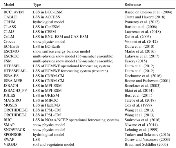
Only climate models will be able to perform the global coupled simulations required for CMIP6, and their land sur-face models will carry out global uncoupled simulations driven with a prescribed meteorological forcing. However, all models – both those that are coupled to an atmospheric model and those that are not (i.e. stand-alone snow models) – can perform the local uncoupled reference site simulations for ESM-SnowMIP at much lower computational expense. Models that have already completed the first round of refer-ence site simulations, listed in Table 1, include land surface schemes (LSS) of CMIP6 models, stand-alone snow physics models, hydrological models, and multi-physics ensemble models.
The experiments proposed in ESM-SnowMIP, with links to relevant LS3MIP reference simulations where appropri-ate, are listed in Table 2 and described in detail in this section. First, we describe single-point experiments, part of which have already been carried out and are currently be-ing analysed. Then, the spatially distributed simulations are described. These latter simulations will be carried out by a subset of the models participating in ESM-SnowMIP, namely global land surface models (LSM) that are also components of an ESM. Finally, we describe planned experiments with land–atmosphere coupling.
3.1 Local scale
3.1.1 Overview of the sites, models, forcing, and evaluation data
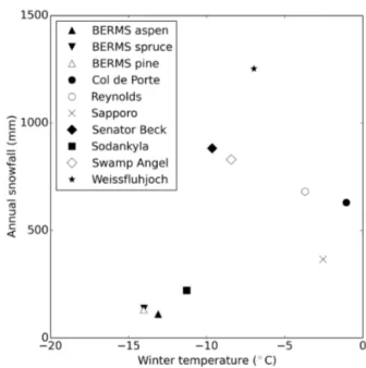
These single-point experiments are enabled by the consid-erable efforts of organizations maintaining the sites to com-pile, quality control, gap fill, and publish their data. Even these reference sites cannot provide all of the input data required by the most sophisticated snow physics models, such as shortwave radiation partitioned into direct and dif-fuse components or aerosol deposition fluxes. Details on the sites used in a first round of ESM-SnowMIP reference site simulations that have already been completed are given in Table 3, and temperature and snowfall statistics are shown in Fig. 1 (the forcing data provide separate rainfall and snow-fall rates). Alpine, Arctic, boreal, and maritime sites have been included in the first round of simulations, and a sec-ond round will introduce tundra and glacier sites. The chal-lenges of maintaining unattended hydrometeorological mea-surements in cold and snowy environments and a require-ment for multiple years of data limit the number of possible sites, but the range of sites and the numbers of years
simu-Figure 1. Winter (DJF) temperatures and annual snowfall averaged over the forcing data periods at the ESM-SnowMIP reference sites (see Table 3).
lated in ESM-SnowMIP far exceed those in similar experi-ments for SnowMIP and PILPS2d.
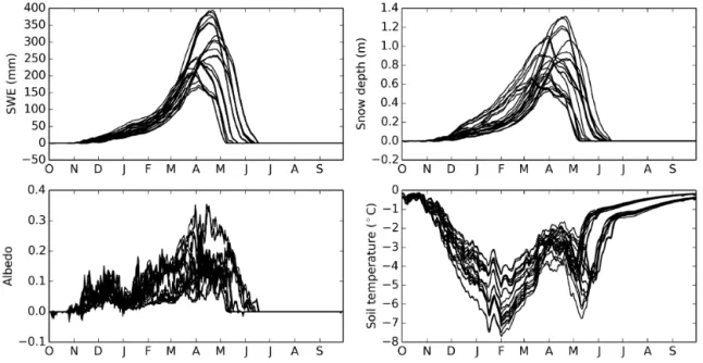
3.1.2 Tier 1: reference site simulations (Ref-Site) Measurements of snow water equivalent (SWE) and depth, and thus also bulk snow density, are available for all of the reference sites. Several sites also have albedo, surface tem-perature, and soil temperature measurements. As examples, Figs. 2 and 3 show measurements and simulations at Col de Porte, which has mild and wet winters, and Sodankylä, which is cold and dry. Observations of SWE, snow depth, surface albedo, and soil temperature are within the model spread and close to the model ensemble means. At the warmer site, the simulations of SWE and depth spread out rapidly as snow accumulates, but most of the soil temperature simulations re-main within a relatively narrow range. Some models have rather low albedos, leading to early melt, and other models melt the snow too late. Apart from a few outliers, SWE sim-ulations at the colder site remain tightly bunched until the spring, but there is a wide spread in winter soil temperature simulations. Some models maintain soil temperatures under snow close to 0◦C, whereas other models are much too cold.
For both sites, there is a strong reduction in model tempera-ture spread as soils cool in autumn before the onset of snow cover and soil freezing.
With several observed variables available for comparison with model outputs and several metrics that can be used for measuring the match between models and observations, there are many ways in which the reference site simulations
Table 1. Models performing ESM-SnowMIP reference site simulations.
Model Type Reference
BCC_AVIM LSS in BCC-ESM Based on Oleson et al. (2004)
CABLE LSS in ACCESS Cuntz and Haverd (2018)
CRHM hydrological model Pomeroy et al. (2012)
CLASS LSS in CanESM Bartlett et al. (2006)
CLM5 LSS in CESM Lawrence et al. (2018)
CoLM LSS in BNU-ESM and CAS-ESM Dai et al. (2003)
Crocus snow physics model Vionnet et al. (2012)
EC-Earth LSS in EC-Earth Dutra et al. (2010)
ESCIMO snow surface energy balance model Marke et al. (2016)
ESCROC multi-physics snow model (35-member ensemble) Lafaysse et al. (2017)
FSM multi-physics snow model (32-member ensemble) Essery (2015)
HTESSEL LSS of ECMWF operational forecasting system Dutra et al. (2012) HTESSELML LSS of ECMWF forecasting system (research) Dutra et al. (2012)
ISBA-ES LSS in CNRM-CM Decharme et al. (2016)
ISBA-MEB LSS in CNRM-CM Boone and Etchevers (2001)
JSBACH LSS in MPI-ESM Roeckner et al. (2003)
JSBACH3_PF LSS in MPI-ESM Ekici et al. (2014)
JULES LSS in UKESM Best et al. (2011)
MATSIRO LSS in MIROC Tatebe et al. (2018)
MOSES LSS in HadCM3 Cox et al. (1999)
ORCHIDEE-E LSS in IPSL-CM Wang et al. (2013)
ORCHIDEE-I LSS in IPSL-CM Wang et al. (2013)
RUC LSS in NOAA/NCEP operational forecasting systems Smirnova et al. (2016)
SMAP snow physics model Niwano et al. (2014)
SNOWPACK snow physics model Lehning et al. (1999)
SPONSOR hydrological model Turkov and Sokratov (2016)
SWAP LSS Gusev and Nasonova (2003)
VEG3D soil and vegetation model Braun and Schädler (2005)
Figure 2. Measurements (red lines), simulations (black lines), and averages of simulations (blue lines) of SWE, snow depth, albedo, and soil temperature at 20 cm of depth for Col de Porte averaged over October 1994 to September 2014.
T able 2. Proposed ESM-Sno wMIP simulations. Configurations are as follo ws. LND 1-D: site-scale 1-D (column); LND: global land simulations with LSMs; LND-A TM-OC: coupled land–atmosphere–ocean simulations. Experiment name T ier Experi ment description and de-sign Configuration Start and end No. years per run Ens. size No. years total Science question and/or g ap ad-dressed with this experiment Possible syner gies with other runs Ref-Site 1 Sit e reference simulations LND 1-D V ariable Ev aluate sno w model on site scale LS3MIP LMIP-H F A-Site 2 Sit e simulations, prescribed constant sno w albedo LND 1-D V ariable Ev aluate ef fect of sno w albedo v ariations Ref-Site NS-Site 2 Sit e simulations, prescribed neutral exchange coef ficient LND 1-D V ariable Quantify ef fect of melt-induced near -surf ace temperature in v er -sions Ref-Site NI-Site 2 Sit e simulations, no soil insula-tion LND 1-D V ariable Diagnose sno w soil insulation ef fect Ref-Site LSF-do wn-scaled-Site 2 Site simulations, do wnscaled forcing LND 1-D V ariable Ev aluate impact of do wnscaled gridded forcing in com ple x to-pograph y Ref-Site SWE-LSM 1 Pres cribed observ ed sno w w a-ter equi v alent LND 1980–2014 35 1 35 Ev aluate link between sno w mass and sno w fraction Land-Hist (LS3MIP) F A-LSM 2 Land-only simulation, pre-scribed constant sno w albedo LND 1980–2014 35 1 35 Ev aluate ef fect of sno w albedo v ariations Land-Hist (LS3MIP) NI-LSM 2 Land-only simulation, no soil insulation LND 1850–2014 165 1 165 Diagnose sno w soil insulation ef fect Land-Hist (LS3MIP) FLC-LSM 2 Land-onl y simulation, pre-scribed common land co v er LND 1980–2014 35 1 35 Diagnose ef fect of v arying pre-scribed land co v ers Land-Hist (LS3MIP) Sno wMIP-rmLC 1 (2) Presc ribed sno w conditions 30-year running mean LND-A TM-OC 1980–2100 121 1 ( + 4) 121 ( + 484) Diagnose sno w–climate feed-back including ocean response CMIP6 historical, Scenario-MIP , LFMIP-rmLC
Table 3. ESM-SnowMIP reference sites with abbreviations used in Fig. 4.
Site Site (short) Latitude Longitude Elevation Period Type Reference
BERMS∗Old Aspen, Canada oas 53.63◦N 106.20◦W 600 m 1997–2010 Boreal Bartlett et al. (2006)
BERMS Old Black Spruce, Canada obs 53.99◦N 105.12◦W 629 m 1997–2010 Boreal Bartlett et al. (2006)
BERMS Old Jack Pine, Canada ojp 53.92◦N 104.69◦W 579 m 1997–2010 Boreal Bartlett et al. (2006)
Col de Porte, France cdp 45.30◦N 5.77◦E 1325 m 1994–2014 Alpine Lejeune et al. (2018)
Reynolds Mountain East, USA rme 43.06◦N 116.75◦W 2060 m 1988–2008 Alpine Reba et al. (2011)
Sapporo, Japan sap 43.08◦N 141.34◦E 15 m 2005–2015 Maritime Niwano et al. (2012)
Senator Beck, USA snb 37.91◦N 107.73◦W 3714 m 2005–2015 Alpine Landry et al. (2014)
Sodankylä, Finland sod 67.37◦N 26.63◦E 179 m 2007–2014 Arctic Essery et al. (2016)
Swamp Angel, USA swa 37.91◦N 107.71◦W 3371 m 2005–2015 Alpine Landry et al. (2014)
Weissfluhjoch, Switzerland wfj 46.83◦N 9.81◦E 2540 m 1996–2016 Alpine WSL (2017)
∗BERMS: Boreal Ecosystem Research and Monitoring Sites.
Figure 3. As Fig. 2, but for October 2007 to September 2014 at Sodankylä (albedo measurements are not available for the snow surface).
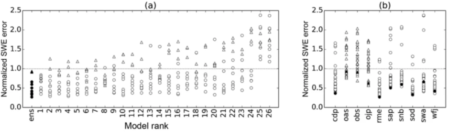
could be evaluated and ranked. Figure 4 shows one exam-ple, in which root mean squared errors in simulated SWE have been calculated for each model at each site and normal-ized by the standard deviation of measured SWE at the given site for comparison between sites. A value greater than 1 for this metric shows that a model fits variations in the observa-tions no better than the average of all observaobserva-tions. Ranking models according to their average error for all sites shows that a couple of models perform well and a couple perform poorly at all sites, but most models perform well at some sites and poorly at others. Many models have larger errors for the forested sites than the open sites and larger errors for warmer sites than colder sites. The ensemble mean of the models has lower errors than the majority of the individual models at most of the sites. The only individual models to have normalized errors less than 1 for all sites are the Cro-cus snow physics model and the HTESSEL and SWAP land surface schemes, which have very different complexity. This
illustrates that model complexity per se does not explain the spread in performance observed here. There will be a thor-ough evaluation of model performance in a forthcoming pa-per.
3.1.3 Tier 2 site simulations
Snow mass balance is influenced by radiated, advected, and conducted heat fluxes in the energy balance. Soil temperature is influenced by snow depth, thermal conductivity, amount of meltwater refreezing, and refreezing depth (van Kampen-hout et al., 2017). To investigate how these influences differ between models, additional experiments are proposed with prescribed snow albedo, with prescribed aerodynamic pa-rameters, and with the thermal insulation of snow removed. These experiments have not started yet, but pilot studies have been conducted using version 2 of the Factorial Snow Model (FSM, Essery, 2015); this is a multi-physics model designed
Figure 4. Normalized root mean square SWE errors for the 26 non-ensemble models in Table 1 returning a single simulation for each site (white symbols) and the 26-model ensemble mean (black symbols), with simulations identified by circles at open sites and triangles at forested sites. (a) Models ranked according to their average error for all sites. (b) Errors for all models at each site (for abbreviations see Fig. 4).
to run ensembles of simulations producing a range of model behaviours by using alternative parameterizations for snow albedo, thermal conductivity, compaction, liquid water stor-age, and coupling with the atmosphere. The pilot studies us-ing FSM allow for the validation of the intended experiment set-up, provide a benchmark for model spread, and facilitate the interpretation of the results.
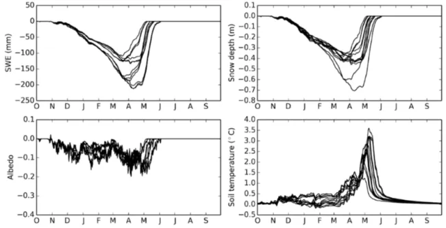
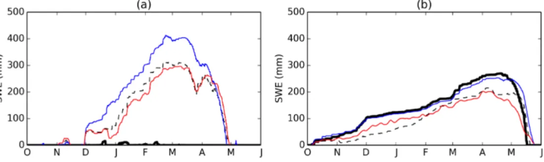
Fixed snow albedo (FA-Site). Seasonal and subseasonal variations of snow albedo are substantial and strongly in-fluence the energy balance of the snowpack. This is partic-ularly important during the melting season when complex processes within the snowpack lead to strong and rapid varia-tions of albedo. Positive albedo feedbacks strongly influence melt timing. Snowmelt timing is a critical climatic metric that is often incorrectly simulated by climate and dedicated snow models, but it is difficult to untangle the effects of the simulation of snow albedo from other processes because of the strong feedbacks involved (Mudryk et al., 2017; Qu and Hall, 2014). An experiment in which snow albedo is fixed to 0.7, which is a typical snow pre-melt albedo (Harding and Pomeroy, 1996; Melloh et al., 2002; Wang et al., 2016), will enable evaluation of the effect of seasonal snow albedo vari-ations and biases.
Differences between an ensemble of fixed snow albedo simulations with FSM and reference simulations for Col de Porte are shown in Fig. 5. Ensemble members differ widely in their responses to the removal of snow albedo feedbacks. Fixing the snow albedo prevents it from decreasing as the snow melts and delays the snowmelt. Extending the duration of snow cover as a result delays warming of the soil in spring, leading to large temperature differences when snow remains in a fixed albedo simulation but has disappeared in the corre-sponding reference simulation.
No suppression of fluxes in stable surface layers over snow (NS-Site).Models generally calculate turbulent heat fluxes in
the atmospheric boundary layer using exchange coefficients that only depend on surface roughness and wind speed in neutral conditions but are reduced in stable conditions by a factor depending on a Richardson number or an Obukhov length. The strength of this decoupling between the atmo-sphere and the surface is a major source of uncertainty in climate and snow models (Schlögl et al., 2017) and will in-fluence how strongly snowmelt responds to warming of the atmosphere. The coupling strength in a model will be quan-tified by an additional experiment in which exchange coeffi-cients are kept fixed at neutral values.
FSM only has a single option for stability adjustment of the surface exchange coefficient, but ensemble members still respond differently to switching this option off, as seen in Fig. 6. Snow-free soil temperatures would also be influenced, so the fix is only applied when snow is on the ground. With heat transfers predominantly being downwards from the at-mosphere to snow, fixing the exchange coefficient increases the heat transfer and warms the snow surface, often leading to decreases in snow albedo and earlier melt. The soil warms rapidly in spring when the snow melts, but winter soil tem-peratures can also be increased relative to the reference sim-ulation despite the decrease in insulating snow depth because of the increased heat flux from the atmosphere.
No thermal insulation by snow (NI-Site). The low ther-mal conductivity of snow has a major climatic control on the temperature of underlying soils and heat fluxes to the at-mosphere that is spatially and temporally variable and often not well represented in climate models (Koven et al., 2013). This insulating effect might be quantified by an experiment in which snow takes a very high (effectively infinite) thermal conductivity, while its other properties (albedo, latent heat of melting, etc.) are kept unchanged. In practice, the numerical scheme of a model might become unstable for high thermal conductivities and another solution might be envisaged, such
Figure 5. Differences between the 32 FSM ensemble members in fixed albedo and reference simulations for Col de Porte averaged over October 1994 to September 2014.
Figure 6. As Fig. 5, but for differences between 16 FSM ensemble members with fixed surface exchange coefficients and 16 with variable coefficients.
as resetting the temperature or the net heat flux at the soil– snow interface to that calculated at the snow surface.
In a pilot study, FSM simulations were found to be numer-ically stable with a fixed 50 W m−1K−1thermal conductivity for snow, which is much higher than a typical range of 0.05 to 0.5 W m−1K−1(Sturm et al., 1997). This value of thermal conductivity led to vanishing temperature gradients across the snowpack and was therefore deemed high enough with-out compromising numerical stability. Results are shown in
Fig. 7. Without the insulating effect of snow, the soil freezes even in the relatively mild winters at Col de Porte. Building up a cold reservoir in the soil over winter has a secondary effect of delaying snowmelt in spring. Even without the in-sulating effect, the high albedo of snow and energy required for snowmelt reduce the amount of energy to warm the soil, leading to a second trough in soil temperature differences be-tween high thermal conductivity and reference simulations.
Figure 7. As Fig. 5, but for differences between the 32 FSM ensemble members in simulations without thermal insulation by snow and reference simulations.
Downscaled large-scale forcing (LSF-downscaled-Site). Most of the mid-latitude ESM-SnowMIP reference sites were established for snow research in mountainous regions and are at higher elevations than much of the surrounding ter-rain. Meteorological variables in large-scale forcing datasets, such as the GSWP3 (Global Soil Water Project Phase 3) meteorological forcing data provided at 0.5◦spatial
resolu-tion for LS3MIP (Kim et al., 2017), would therefore be ex-pected to be biased relative to in situ measurements at the sites even if they were perfect on the grid scale. Col de Porte, for example, is located at an elevation of 1325 m in the French Chartreuse Mountains but lies within a 0.5◦grid cell with an average elevation of 870 m. Figure 8a shows that an FSM simulation for winter 2009–2010 at Col de Porte with GSWP3 driving data gives almost no snow accumula-tion; this is because temperature on the grid scale, because of the lower mean altitude, is higher than at Col de Porte, while total precipitation is lower and snowfall is much lower. Site and grid elevations for Sodankylä, in contrast, only differ by 40 m because this site is situated in a flat area. The large-scale simulation shown in Fig. 8b is not so strongly influenced by driving data biases.
Downscaling is commonly required when using regional climate predictions in hydrological impact studies. An ESM-SnowMIP experiment with altitude-adjusted large-scale driv-ing data will be helpful in usdriv-ing reference site observations and simulations to evaluate the performance of models in large-scale simulations. Simply removing average altitude-related errors in the GSWP3 driving data, with no attempt to adjust variations on interannual and shorter timescales, greatly improves the SWE simulation for Col de Porte,
re-placing a massive underestimate with a slight overestimate (Fig. 8a). For Sodankylä, removing the smaller long-term driving data biases has very little effect on the SWE simu-lation (Fig. 8b).
We expect the Tier 2 site simulations with the individual models to essentially align with the FSM results presented here. However, we also expect a varying degree of sensitiv-ity of the various models to the different model parameter and set-up changes, which will allow for the identification of unique priorities for the development of each of the partici-pating models.
3.2 Global scale
3.2.1 Large-scale observational data
Observation-based estimates of SWE and snow cover frac-tion (SCF) are required for the evaluafrac-tion of historical mean and model spread from ESM-, AMIP-, and LMIP- type simulations, as well as prescribed historical SWE and SCF as required for specific experiments. For this purpose, we will employ a blended dataset of snow products from ERA-Interim/Land (Balsamo et al., 2015), MERRA (Rienecker et al., 2011), ERA-Crocus (Brun et al., 2013), ESA-GlobSnow (Takala et al., 2011), and GLDAS-2 (Rodell et al., 2004). These SWE datasets were assessed previously for temporal and spatial consistency by Mudryk et al. (2015), who pro-posed a climatology derived from a combination of these five datasets.
The rationale for using a blended suite of snow products is threefold. First, it provides a measure of historical observa-tional uncertainty given by the range of estimates from
indi-Figure 8. Simulations with a single FSM ensemble member and in situ driving data (dashed black lines), large-scale GSWP3 driving data (solid black lines), or bias-corrected GSWP3 driving data (blue lines) compared with in situ SWE measurements (red lines) for 2009–2010 at (a) Col de Porte and (b) Sodankylä.
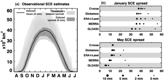
Figure 9. Daily median and spread (5th–95th percentile) among the five snow products listed above for the 1981–2010 period.
vidual analyses. This is demonstrated in Fig. 9, which shows the daily median and spread (5th–95th percentile) among the five snow products listed above for the 1981–2010 seasonal SWE climatology. For a given day, statistics are calculated from the pooled distribution of data across the 30-year pe-riod and across all five datasets. As analysed in Mudryk et al. (2015), the range across the snow products likely results from differences in the snow schemes within the land sur-face models, differences in precipitation and temperature in the forcing meteorology (from various reanalyses), and the impact of satellite and weather station measurements (used in GlobSnow and ERA-Brown). Still, the illustrated spread is a useful proxy for observation-based uncertainty (which cannot be determined when a single product is applied for evaluation) and may be used to evaluate the corresponding level of agreement from LS3MIP and ESM-SnowMIP simu-lations over a similar historical period.
A second reason to use a suite of analyses for MIP evalua-tion is that the bias and error of individual datasets vary with geographical location and datasets that perform well in some regions may perform more poorly in others. The lack of a
clear “best” dataset provides minimal reason to favour one analysis over another. In fact, it has been explicitly demon-strated that combinations of products have both lower bias and RMSE than individual products when evaluated over do-mains with in situ data (Schwaizer et al., 2016). For this rea-son, a blended combination of snow products will be used for time-varying prescribed SWE simulations (see Sect. 3.2.2) and could also be used for evaluation of SWE output from simulations which are observationally constrained by non-snow-related variables.
Finally, the use of SWE analyses also allows for the defini-tion of a mutually consistent set of snow cover extent (SCE) data by choosing a seasonal and climatological SWE thresh-old above which a grid cell is considered snow-covered. The spread of total NH SCE estimated from a range of thresholds between 0 and 10 mm is large (Fig. 10a; light shading) with much of the uncertainty related to very low SWE thresholds (< 2 mm), for which reanalysis-based SWE persists on the land surface for physically unrealistic amounts of time. Op-timization based on satellite-based observations of climato-logical SCE has identified 5 mm as a reasonable choice of threshold (Fig. 10a; dark shading) for deriving SCE from SWE (Robinson et al., 2014).
3.2.2 Global land-only simulations
The global land-only simulations planned in ESM-SnowMIP build on the reference historical land simulation (Land-Hist) currently carried out in the framework of the LS3MIP project. The aim of this 1850–2014 simulation, using GSWP3 meteorological forcing, is to provide a land-only simulation carried out with the land surface modules used in the CMIP6 ESMs at the same resolution as used in the cou-pled model, allowing for the separate evaluation of the land surface components of these models and potentially attribut-ing sources of coupled model biases to the individual coupled model components. The global land simulations planned in ESM-SnowMIP share the model set-up with this Land-Hist simulation to optimize complementarity.
Figure 10. (a) Daily median and spread (5th–95th percentile) among the five snow products for SCE calculated using a 5 mm SWE threshold (solid curve and dark shading) and spread calculated using a range of thresholds between 0 and 10 mm (light shading). (b) January and May SCE for four choices of thresholds.
Tier 1: prescribed observed snow water equivalent (SWE-LSM).The relationship between grid-scale snow water equiv-alent (SWE), fractional snow cover, and hence surface albedo is complicated and very diverse solutions are presently im-plemented in coupled climate models. Here we propose a prescribed SWE experiment to identify LSM biases that are linked to the parameterization of surface albedo as a func-tion of the snow cover fracfunc-tion, which in turn is very often a diagnostic function of the SWE which is prescribed in this experiment. The aim is to evaluate the simulated grid-scale albedo in these simulations against satellite-based observa-tions of surface albedo.
Simulated grid-scale surface albedo in the presence of snow can depend explicitly on subgrid-scale topography, pa-rameterized patchiness, vegetation cover, snow albedo, and other factors. The vegetation cover dependence includes ex-plicitly simulated masking of vegetation by snow or vice versa. In particular, the albedo effect of transient snow load on trees after snowfall with subsequent unloading due to wind and melting, which is sometimes represented in current-generation ESM snow modules, should not be off-set by too simple a prescription of observed SWE. It should therefore be left up to the modelling groups to decide exactly how SWE is prescribed in their models. However, the model SWE should satisfy the condition that the weekly average SWE in the model is close to the observed value (by less than 10 %). This can, for example, be obtained by a Newto-nian relaxation of SWE to the weekly average with a time constant of a few days. Other state variables of the snow module (e.g. snow internal temperature, water content, snow grain size, etc.) will have to be adapted accordingly; again, given the diversity of snow modules, it is impossible to define here exactly how this needs to be done in general. Note that these considerations also apply for the land-only simulations of LS3MIP in which soil wetness and SWE are to be
pre-scribed. In cases of snow modules for which an unequivocal relationship ties surface albedo to SWE, it might be sufficient to run only the albedo scheme with prescribed SWE as input. While a number of snow products are available to serve as prescribed SWE, we recommend the Mudryk et al. (2015) combined climatology (see Sect. 3.2.1) for ESM-SnowMIP simulations. Because biases in individual products are com-pensated for through averaging, this dataset represents an improved reference for model evaluation compared to any single-component dataset (Sospedra-Alfonso et al., 2016), just like a climate model ensemble mean is often preferred over a single member.
The simulated surface albedo will be compared to sur-face albedo as derived from satellite observations (MODIS, Schaaf et al., 2002; APP-x, Wang and Key, 2005; Glob-Albedo, Lewis et al., 2012). In particular, the change in the quality of the simulated surface albedo compared to the “free” LS3MIP Land-Hist simulation and the historical CMIP6 simulation will be evaluated in order to infer the part of surface albedo errors linked to a biased snow mass bal-ance.
Tier 2: fixed snow albedo (FA-LSM).This is a spatially dis-tributed version of the FA-Site simulation described above. It consists of prescribing snow albedo to a fixed value of 0.7. The aim of the experiment is, similar to that of the FA-Site simulation, to enable evaluation of the effect of seasonal snow albedo variations and biases in LSMs, although the model response will depend very much on how snow mask-ing by vegetation is parameterized.
Simulated snow water equivalent (SWE), fractional snow cover, and vegetation masking will still influence the grid-point average surface albedo. The simulation period is 1980– 2014, as in the Land-Hist and SWE-LSM simulations. If pos-sible, the fixed snow albedo value should also be used over ice sheets. Correct prescription of snow albedo can be
ver-ified by checking grid-scale average surface albedo in ar-eas with deep snow cover and low vegetation. In addition, the effect of vegetation masking on surface albedo in snow-covered areas will be isolated, since the snow–vegetation pa-rameterizations will vary between models, but snow albedo will remain fixed.
This simulation is tightly linked to the LS3MIP Land-Hist offline reference simulation. In synergy with the site sim-ulation with prescribed snow albedo (FA-Site), comparison with the same period in the reference simulation allows for the evaluation of the effect of snow albedo in terms of tim-ing of snowmelt, winter season surface temperature, and en-ergy flux partitioning as a source of model biases. In addition, the effect of vegetation masking on surface albedo in snow-covered areas will be isolated, since the snow–vegetation pa-rameterizations will vary between models, but snow albedo will remain fixed. Again, as in FA-Site, a basic metric to eval-uate the effect of prescribed snow albedo will be the dura-tion of snow cover (in particular melt onset) in this experi-ment compared to the reference simulation and observation. Required observations therefore concern snow cover season-ality, in particular snowmelt dates (to be obtained from the ensemble of large-scale SCE data), and general climate vari-ables such as surface air temperature.
Tier 2: no thermal insulation by snow (NI-LSM).We pro-pose a global LSM simulation with “infinite” snow conduc-tivity (that is, no effective thermal insulation by snow) as a global extension of the site-scale experiment NI-Site. Again, this simulation will otherwise have an identical set-up as the relevant reference simulation Land-Hist. However, the mod-els might need to be spun up for a substantial number of years in this set-up in order to achieve thermal equilibrium at the lowest soil levels.
In this global setting, simulated potential permafrost extent (that is, the permafrost extent in equilibrium with the pre-scribed climate and model set-up, also often termed “near-surface permafrost”; e.g. Lawrence et al., 2008) will be di-agnosed from the thermal state of the lowermost soil layer in the simulations. It will be compared to the correspond-ing output of the Land-Hist reference simulation and GTN-P observations (Biskaborn et al., 2015). Required reference data are soil temperature measurements and observations and analyses of surface energy fluxes at all seasons in areas with seasonal snow cover. Again, in the multi-model context, we expect a relationship between the sensitivity of the simulated potential permafrost extent to thermal insulation by soil and diagnosed errors of the simulated near-surface permafrost ex-tent, which we hope will be useful to identify ways for model improvement.
Tier 2: fixed land cover (FLC-LSM).Previous studies show that inaccurate representation of vegetation distribution and parameters in LSMs may result in large biases in simulated surface albedo for snow-covered forests (Essery, 2013; Wang et al., 2016). Most current LSMs represent vegetation from a set of plant functional types (PFTs), which are usually
de-rived from global land cover datasets (Bonan et al., 2002; Poulter et al., 2015). There are large differences among PFTs used in LSMs, which may result from the differences in the land cover datasets, the cross-walking tables used to map land cover datasets into PFTs represented in LSMs, or un-certainties in dynamic PFT simulations (Hartley et al., 2017; Poulter et al., 2011). In order to separate biases due to dif-ferences in vegetation distribution from those due to physi-cal processes in LSMs, we propose an experiment in which models derive their PFTs from the same land cover dataset and using the same cross-walking table.
Several global land cover datasets are available with spa-tial resolutions ranging from 300 m to 1 km (Bontemps et al., 2012). The newly released European Space Agency (ESA) Climate Change Initiative (CCI) land cover datasets are de-veloped specifically to address the needs of the climate mod-elling community (Poulter et al., 2015). The CCI maps in-clude 22 level-1 classes and 15 level-2 subclasses based on the United Nations Land Cover Classification System, which was identified as a suitable thematic legend and compati-ble with the PFT concept of most LSMs (Bontemps et al., 2012). While most previous land cover datasets are for a sin-gle year, the CCI datasets are available from 1992–2015 at 300 m resolution (ESA, 2017). The finer spatial resolution of 300 m (versus 1 km) makes it inherently superior for land cover mapping in heterogeneous landscapes for which dif-ferent datasets tend to disagree (Fritz et al., 2011; Herold et al., 2008). In addition, a cross-walking table to convert the categorical land cover classes to the fractional area of PFTs was provided with the CCI datasets (Poulter et al., 2015). We thus suggest the use of the CCI land cover dataset for the year 2000 as the common land cover dataset from which to derive PFTs. Different models usually have their own unique set of PFTs. For cases in which both the phenology type and the associated climate zone are considered, the Köppen–Geiger climate classification can be used as in Poulter et al. (2015).
The simulation period of 1980–2014 matches the LS3MIP Land-Hist offline reference simulations. A comparison of the surface albedo with the reference simulation will isolate the impact of PFT distribution on surface albedo and associ-ated feedbacks in snow-covered areas. Since the PFTs are from the same land cover data in the participating models, the differences in surface albedo among the models will re-veal differences in snow–vegetation interactions and other vegetation-related parameterizations (e.g. leaf area index) used in the models.
3.2.3 Global simulation with land–atmosphere coupling: SnowMIP-rmLC
ESM-SnowMIP proposes one coupled Tier 1 experiment, which serves the purpose of quantifying snow-related feed-backs in the global climate system on interannual timescales. It is designed to separate the effects of snow from the effects of snow and soil humidity, the combined effect being
ad-dressed by the LS3MIP Tier 1 coupled experiment LFMIP-rmLC. This LS3MIP experiment uses 30-year running mean land conditions (snow and soil humidity), as simulated in a reference transient climate change experiment, and pre-scribes these in a second simulation. In these runs, snow and soil moisture feedbacks on decadal and shorter timescales are muted. Comparing the LFMIP-rmLC simulation to the appropriate projection used for prescribing the land surface conditions allows for the identification of these feedbacks. In the context of a transient run, additional diagnoses of geo-graphic shifts of land–atmosphere coupling hotspots (Senevi-ratne et al., 2006) and changes in potential predictability re-lated to land surface (Dirmeyer et al., 2013) can be carried out. The SnowMIP-rmLC will isolate the effects of snow– atmosphere coupling by prescribing only the soil humidity state from the reference simulation, not the entire surface state as in LFMIP-rmLC.
For the SnowMIP-rmLC experiment, the LFMIP-rmLC experiment set-up is modified such that only the climatologi-cal soil humidity is prescribed. Contrary to the LFMIP-rmLC experiment, snow is allowed to evolve freely. The rationale behind this choice is that in this way, our simulation set-up is more similar to previous GLACE–CMIP experiments (Seneviratne et al., 2013), while the effect of snow can be deduced from the difference between these two simulations. Because of internal variability in the climate system, a five-member ensemble simulation would be ideal, but this is ex-pensive. Similar to the LFMIP-rmLC set-up, we propose the first ensemble member as Tier 1 and suggest four other en-semble members as Tier 2 (see Table 2). The simulation pe-riod is the same as in LFMIP-rmLC, i.e. 1980–2100. Cor-rect prescription of snow can be verified easily by comparing the simulated SWE for an individual year with the simulated climatological (1980–2014) SWE of the free projection. It should be very close.
The SnowMIP-rmLC experiments will allow for the eval-uation of the effect of snow feedbacks on interannual to decadal timescales as well as on the centennial climate change signal (since even by the end of the 21st century, the 1980–2014 average snow conditions will be used).
The simulation will be analysed in parallel to the LFMIP-rmLC simulations, following very closely the methodologies of Seneviratne et al. (2013). Required observations are snow cover seasonality, in particular snowmelt dates, and general climate variables such as surface air temperature, and circu-lation patterns.
3.2.4 Snow shortwave radiative effect diagnosis Another useful measure of the impact of snow on climate is the snow shortwave radiative effect (SSRE) (e.g. Flanner et al., 2011; Perket et al., 2014; Singh et al., 2015). For the purposes outlined here, SSRE is the instantaneous change in surface absorbed solar energy flux caused by the pres-ence of terrestrial snow. The diagnosis of SSRE provides a
precise, overarching measure of the snow-induced perturba-tion to solar absorpperturba-tion in each model, integrating over the variable influences of vegetation masking, snow grain size, snow cover fraction, soot content, and other factors. SSRE is also a useful measure for climate feedback analysis and has a direct analogue in the widely used “cloud radiative ef-fect”. To enable us to calculate and analyse inter-model dif-ferences of SSRE and their causes, participating modelling groups are requested to provide specific gridded output (see below) from their LS3MIP Land-Hist and Land-Future sim-ulations, as well as from the ESM-SnowMIP FA-LSM and SWE-LSM simulations. Ideally, these output fields should also be provided for one or more of the coupled atmosphere– ocean simulations, preferably from the historical reference run.
SSRE can be calculated in a land surface model through the following procedures.
1. Conducting an additional surface albedo calculation at each model time step with zero snow. This implies set-ting to zero the mass of snow on ground, mass of snow in vegetation canopy, and snow cover fraction, but only for the purpose of this diagnostic albedo calculation. It should have no effect on the prognostic snow simula-tion.
2. Calculating net and reflected surface solar energy fluxes at each model time step using the diagnostic albedo from (1) and using the same surface downwelling (in-cident) flux that would otherwise be used to calculate solar heating.
3. Archiving the diagnostic calculations from (1) and (2) at the same frequency as other model output (e.g. daily or monthly).
The following gridded fields should be provided from the model: (1) net surface shortwave irradiance calculated with-out snow (rss_ nosno); and (2) mean shortwave surface albedo calculated without snow (albs_nosno).
Net surface solar energy flux in the absence of snow can then be differenced from that calculated with snow (output by default) to provide the SSRE.
Although the no-snow albedo fields are not strictly needed for the calculation of SSRE, they will complement standard albedo output from the model to facilitate convenient evalu-ation and the derivevalu-ation of hypothetical SSRE from different (e.g. clear-sky) surface downwelling irradiance fields. De-pending on the spectral resolution of solar energy in each model, it would also be useful to provide the visible and near-infrared partitions of the following: (1) net surface visi-ble (0.2–0.7 µm) irradiance calculated without snow; (2) net surface near-IR (0.7–5.0 µm) irradiance calculated without snow; (3) mean visible surface albedo calculated without snow; and (4) mean near-IR surface albedo calculated with-out snow.
3.3 Timeline, data request, and data availability The first set of reference site simulations (Ref-Site) have al-ready been carried out and are currently being analysed. The additional site simulations will be carried out in the near fu-ture. In 2018 and 2019, the global climate modelling com-munity will be heavily involved in CMIP6. To decrease peak workload on the modelling groups while at the same time optimizing synergies with the CMIP6 activities and in par-ticular with LS3MIP, it was decided to launch the ESM-SnowMIP simulations after the main CMIP6 activities. This, however, has the disadvantage that ESM-SnowMIP global simulation results will not be available for analysis in time for the sixth IPCC assessment report.
For these global land-only and coupled simulations, the request for output variables is identical to the LS3MIP data request (https://www.earthsystemcog.org/projects/wip/ CMIP6DataRequest, last access: 3 December 2018) for the respective reference simulations indicated in Table 2, and the model set-up will be very similar, as described in the preced-ing sections of this paper. This further keeps the additional workload for the ESM-SnowMIP coupled simulations to a minimum.
The ESM-SnowMIP site simulation output is sufficiently small to be easily handled via an ftp server at one of the participating institutes (see the dedicated website at https: //www.geos.ed.ac.uk/~ressery/ESM-SnowMIP.html, last ac-cess: 3 December 2018). Gridded Northern Hemisphere SWE data are freely available from the National Snow and Ice Data Center (http://nsidc.org/data/NSIDC-0668, last ac-cess: 3 December 2018). Large-scale meteorological forc-ing (GSWP3) for the distributed simulations, also used in LS3MIP, will be made available via the ESGF at https: //esgf-node.llnl.gov/search/input4mips/ (last access: 3 De-cember 2018). To optimize synergies with LS3MIP, ESM-SnowMIP will seek endorsement by the WCRP Working Group on Coupled Modelling, which oversees CMIP. This will allow ESM-SnowMIP output to be handled via the Earth System Grid Federation (https://esgf.llnl.gov/, last access: 3 December 2018), i.e. the same infrastructures as the rel-evant CMIP6 simulations these simulations are to be com-pared with.
4 Discussion
4.1 Expected outcome and impact of ESM-SnowMIP The parameterization of “cold” land surface processes has received varying degrees of attention by climate modelling groups. In the framework of CMIP6, there is now a specific type of numeric experiment specifically designed for evalu-ating the land surface components of the current-generation Earth system models. It is envisaged that these so-called LMIP exercises could become a central component of future
CMIP editions as part of the so-called DECK core experi-ments (Eyring et al., 2016), along with separate evaluations of the atmospheric and ocean components.
The specific effort aiming at evaluating and improving the representation of snow in ESMs and in more specific dedi-cated snow models relates to this broader context. It is hoped that ESM-SnowMIP, in conjunction with LS3MIP, will pro-vide a clear determination of the current state of the art of snow modelling in the different participating communi-ties and will spur knowledge transfer between these partially disjointed scientific communities. Snow modules in current-generation ESMs show a wide spread in their degree of com-plexity. We expect that ESM groups who have not devoted particular effort to evaluating and improving their snow mod-ules in the past will be able to benefit from a clear strategy for priorities of first-order snow module enhancements iden-tified within ESM-SnowMIP. For groups that have already put substantial effort into testing and continuously adapting their ESM snow modules or specific snow models, ESM-SnowMIP will be an opportunity to assess past and determine future priorities for model enhancement.
The intended assessment of snow-related feedbacks on in-terannual and longer timescales, such as a multi-model eval-uation of the snow shortwave radiative effect, will hopefully help better constrain the global climate response to anthro-pogenic forcing and better understand regional responses, in-cluding the amplification of global warming at high northern latitudes.
4.2 Possible actions for future follow-up projects Recent work on tundra snow (Domine et al., 2016) has high-lighted the importance and specificity of snow metamorphic processes under very cold conditions, specifically in the pres-ence of strong vertical temperature gradients. While wind compaction in the absence of shelter by higher vegetation can increase snow density (Sturm et al., 2001) and hence snow conductivity, depth hoar formation induced by strong vertical temperature gradients within the snowpack (Derksen et al., 2009, 2014) can substantially reduce the conductiv-ity (Domine et al., 2016). In ESM-SnowMIP, an effort will be made to include snow observation sites from tundra en-vironments in the near future (e.g. Boike et al., 2018). How-ever, it is clear that in future extensions of ESM-SnowMIP, snow on sea ice and on the polar ice sheets should also be-come a focus of attention. The physical properties of snow on sea ice are linked to low accumulation rates and strong ver-tical temperature gradients due to bottom heat flux, its spa-tial heterogeneity, its peculiar evolution in summer leading to melt ponds on sea ice due to inhibited drainage of meltwater, and the presence of salt. These are specificities that are, to our knowledge, often not taken into account in Earth system models; however, snow on sea ice obviously concerns the sea ice module of the coupled models and thus a slightly different community than that mobilized in this first version of
ESM-SnowMIP. Assessments of snow on sea ice usually focus on, and are usually limited to, snow mass and height (Blanchard-Wrigglesworth et al., 2015; e.g. Hezel et al., 2012). However, an extension of the ESM-SnowMIP approach based on com-bined small- and large-scale evaluation of snow models will necessarily be conditioned by the availability of high-quality observations. In this context, the MOSAIC international Arc-tic drift expedition (https://www.mosaic-expedition.org/, last access: 3 December 2018) is projected to provide valuable new observations.
A further obvious follow-up of ESM-SnowMIP could tackle snow in extreme polar environments such as Dome C on the East Antarctic Plateau or the Greenland Summit; long-term meteorological observations have already been used at these locations for testing stand-alone snow models (Car-magnola et al., 2013; Libois et al., 2015). Perennial snow cover evolving under such extreme conditions would sub-stantially broaden the range of snow types evaluated within our framework. This would provide stringent tests for snow models designed to simulate snow types that are extreme but far from rare, as the interior regions of the continental polar ice sheets make up an essential part of the perennial cryosphere.
ESM-SnowMIP combines model evaluation at local and global scales. While snow, and particularly the timing and intensity of its melt season, does have important effects on basin-scale hydrology (Barnhart et al., 2016; e.g. Berghuijs et al., 2014; Fyfe et al., 2017), basin-scale processes exert a less dominant control on snow as such in terms of physi-cal properties. Therefore, intermediate sphysi-cales, such as those addressed in the Rhône-Aggregation Land Surface Scheme Intercomparison Project (Boone et al., 2004), are bridged in the current phase of ESM-SnowMIP. However, terrain con-figuration and vegetation distribution (that is, geographical characteristics at intermediate (basin) scales) have an obvi-ous and important effect on the snow cover, in particular on snow cover fraction. In the current phase of ESM-SnowMIP, such links are implicitly addressed through the assessment of snow cover fraction in the prescribed SWE experiment SWE-LSM. In future phases, basin-scale properties, processes, and characteristics might be addressed more explicitly. A fur-ther aspect involving unresolved scales that could be tack-led in future extensions of ESM-SnowMIP is the high spatial variability of impurities deposited on snow surfaces, given the known strong impact of this deposition on snow albedo (Flanner et al., 2007) and model errors that can be induced by not taking this effect into account (e.g. Clark et al., 2015).
Data availability. Site forcing data are available through https: //www.geos.ed.ac.uk/~ressery/ESM-SnowMIP/netcdf.zip (last ac-cess: 7 December 2018). The Weissfluhjoch data are accessible via https://doi.org/10.16904/16 (WSL, 2017). A paper describing the site-scale input data is currently in preparation.
Author contributions. GK, CD, RE, MF, SH, MC, AH, and HR ini-tially designed the experimental design. GK, CD, RE, CBM, LM and LW led the initial writing of different parts of the paper. RE and CBM led the analysis of the site simulations. All other participants contributed to the final experimental design, the site simulations and the projected analysis strategy.
Competing interests. The authors declare that they have no conflict of interest.
Acknowledgements. This project was supported by the World Climate Research Programme’s Climate and Cryosphere (CliC) core project. We acknowledge the World Climate Research Programme’s Working Group on Coupled Modelling, which is responsible for CMIP. For CMIP the U.S. Department of Energy’s Program for Climate Model Diagnosis and Intercomparison provides coordinating support and led the development of software infrastructure in partnership with the Global Organization for Earth System Science Portals. Analysis of ESM-SnowMIP reference site simulations is supported by NERC grant NE/P011926/1. Gerhard Krinner, Chris Derksen, and Richard Essery acknowledge support by the ESA in the framework of the ESA CCI snow project. Simulations by the SWAP model were supported by the Russian Science Foundation (grant 16-17-10039; Yeugeniy M. Gusev is the recipient). Simulations by the SPONSOR model were supported by the Russian Foundation for Basic Research (grant 18-05-60216; Vladimir A. Semenov is the recipient). The work of Gabriele Ar-duini leading to this paper was funded through the APPLICATE project. APPLICATE has received funding from the European Union’s Horizon 2020 research and innovation programme under grant agreement 727862. Nander Wever was supported by the Swiss National Science Foundation (project 200021E-160667). IGE and CNRM/CEN are part of LabEX OSUG@2020 (ANR10 LABX56). Stefan Hagemann and Tobias Stacke were partially supported by funding from the European Union within the Horizon 2020 project CRESCENDO (grant no. 641816). Hyungjun Kim acknowledges support by a Grant-in-Aid for Specially Promoted Research 16H06291 from JSPS. Alex Hall was supported by the U.S. National Science Foundation under grant number 1543268: “Reducing Uncertainty Surrounding Climate Change Using Emergent Constraints”. The authors sincerely thank Eric Brun-Barrière for his leading role during the initial planning stages of ESM-SnowMIP.
Edited by: Jeremy Fyke
Reviewed by: two anonymous referees
References
Balsamo, G., Albergel, C., Beljaars, A., Boussetta, S., Brun, E., Cloke, H., Dee, D., Dutra, E., Muñoz-Sabater, J., Pappen-berger, F., de Rosnay, P., Stockdale, T., and Vitart, F.: ERA-Interim/Land: a global land surface reanalysis data set, Hydrol. Earth Syst. Sci., 19, 389–407, https://doi.org/10.5194/hess-19-389-2015, 2015.