HAL Id: hal-01168394
https://hal.inria.fr/hal-01168394
Submitted on 25 Jun 2015
HAL is a multi-disciplinary open access
archive for the deposit and dissemination of
sci-entific research documents, whether they are
pub-lished or not. The documents may come from
teaching and research institutions in France or
abroad, or from public or private research centers.
L’archive ouverte pluridisciplinaire HAL, est
destinée au dépôt et à la diffusion de documents
scientifiques de niveau recherche, publiés ou non,
émanant des établissements d’enseignement et de
recherche français ou étrangers, des laboratoires
publics ou privés.
Planar Shape Detection and Regularization in Tandem
Sven Oesau, Florent Lafarge, Pierre Alliez
To cite this version:
Sven Oesau, Florent Lafarge, Pierre Alliez. Planar Shape Detection and Regularization in Tandem.
Computer Graphics Forum, Wiley, 2015, pp.14. �hal-01168394�
Planar Shape Detection and Regularization in Tandem
Sven Oesau Florent Lafarge Pierre Alliez
Inria Sophia Antipolis - Méditerranée, France
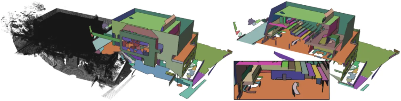
Figure 1: Shape detection and regularization. The input point set (5.2M points) has been acquired via a LIDAR scanner, from the inside and outside of a physical building. 200 shapes have been detected, aligned with 12 different directions in 179 different planes. The cross section depicts the auditorium in the upper floor and the entrance hall in the lower floor. The closeup highlights the steps of the auditorium which are made up of perfectly parallel and orthogonal planes.
Abstract
We present a method for planar shape detection and regularization from raw point sets. The geometric modeling and processing of man-made environments from measurement data often relies upon robust detection of planar primitive shapes. In addition, the detection and reinforcement of regularities between planar parts is a means to increase resilience to missing or defect-laden data as well as to reduce the complexity of models and algorithms down the modeling pipeline. The main novelty behind our method is to perform detection and regularization in tandem. We first sample a sparse set of seeds uniformly on the input point set, then perform in parallel shape detection through region growing, interleaved with regularization through detection and reinforcement of regular relationships (coplanar, parallel and orthogonal). In addition to addressing the end goal of regularization, such reinforcement also improves data fitting and provides guidance for clustering small parts into larger planar parts. We evaluate our approach against a wide range of inputs and under four criteria: geometric fidelity, coverage, regularity and running times. Our approach compares well with available implementations such as the efficient RANSAC-based approach proposed by Schnabel and co-authors in 2007.
1. Introduction
Shape detection from 3D point clouds is a multi-faceted problem aimed at explaining data by discovering primitive shapes. Turning a large amount of raw sampling data into a higher-level representation also leads to complexity reduc-tion and hence yields more practical algorithms for appli-cations. Object classification methods can learn information from labeled collections of primitive shapes in order to cat-egorize new unknown objects by comparison. Entire scenes can be analyzed via the arrangement of classified objects and
shapes, e.g., for classifying objects in indoor environments [KAJS11] or recognizing specific structures [VGSR04]. Sur-face reconstruction methods for objects or entire scenes also benefit from a collection of primitive shapes that brings use-ful geometric priors in interactive, e.g., [SSS∗08,ASF∗13], and automatic, e.g., [SDK09,LA13], contexts. For urban or indoor reconstruction in particular, primitive shape detection is commonly performed as first step [MWA∗13]. Primitive shapes are also amenable to the meaningful recovery of hid-den or missing parts of objects. The arrangement of
prim-itive shapes is often used to infer the semantics from raw measurement data.
Beyond detection of the shapes themselves, one more step is to detect the regular relationships (regularities) between the shapes and to reinforce them - a process referred to as regularization. Due to practical reasons and manufacturing constraints, man-made objects and environments are often compositions of primitive shapes and exhibit a large num-ber of regularities such as parallel, coplanar and orthogonal relationships. When dealing with defect-laden and missing data, an increasing number of reconstruction methods rely upon these regularities when deriving the surfaces from a collection of shapes. Some shape detection approaches al-ready consider domain-specific information by, e.g., favor-ingapproximate regularities. However, only the exact reg-ularity of the detected shapes has substantial impact upon the complexity of the algorithms downstream the model-ing pipeline. For, e.g., reconstruction approaches proceed-ing by space partitionproceed-ing, coplanar and parallel primitives reduce significantly both the number of cells of the parti-tion and the overall visual complexity of the reconstructed scenes [CLP10].
In this work we focus on the automated detection and regularization of primitive shapes from unorganized point clouds. Point cloud is the de facto standard data format for surface reconstruction methods and can be generated from laser scanners, structured light cameras such as Kinect, or multi-view stereo. We further focus on planar primitive shapes as our man-made environment is mostly composed of planar parts, and parts of curved surfaces can be approxi-mated with smaller planar shapes (Figure1). We consider the 3 main relationships (parallelism, orthogonality and copla-narity) that form the major regularities in urban scenes and can reinforce detection by non-local fitting. Covering more of the many possible regularities such as equidistant place-ment and co-angularity would introduce more conflicts be-tween relationships and thus negatively impact data fidelity. 1.1. Previous work
Shape detection. The automated detection of primitive shapes is an instance of the general problem of fitting mathematical models to data. There is a wide variety of shapes in all dimensions, the simplest example in the early days of Computer Vision being the detection of 1D shapes such as line segments in 2D images. The rapid technological advances and affordability that characterized the acquisition devices have stimulated research for detecting 2D shapes in 3D point clouds. Furthermore, the detection of 3D shapes such as cuboids in images [XRT12] is used to understand the arrangement of 3D objects in indoor scenes. We review next several shape detection approaches for measurement data.
RANSAC. The random sample consensus (RANSAC)
[FB81] has been widely used for shape detection, e.g. [SHFH11]. Based on stochastic sampling and probabilities, it constructs iteratively many shape hypotheses from few samples and verifies them against the input data in order to select the shapes with highest number of inliers. In addition to being a non-deterministic algorithm, RANSAC only pro-duces satisfactory results with a probability that depends on the number of iterations. The latter is potentially huge as it depends on, e.g., the number of triplets of points required to determine a 3D plane. Schnabel et al. [SWK07] proposed a fast RANSAC-based method for detecting several types of primitive shapes in point-cloud data. This approach is sat-isfactory in particular when the shapes are heterogeneous in size, as it optimizes for the probability to not miss the largest shapes. It is however less efficient on large-scale ur-ban scenes containing a large number of small shapes.
Hypothesis-then-selection. As for RANSAC this
ap-proach generates many hypotheses from the input data. In a subsequent step labeling is performed to assign one hypoth-esis to each input sample while minimizing a global energy designed to, e.g., favor regularity. Pham et al. [PCYS12] ap-plied this approach to homography detection in images using graph-cut for energy minimization.
Accumulation space. Accumulation space methods rely upon voting in parameter space of the shapes sought after. Many primitive shape hypotheses are locally fitted to data samples and accumulated in parameter space. The final shapes are extracted via clustering of the corresponding density function in parameter space, through, e.g., mean shift [Che95]. The Hough transform is a common accumu-lation space method [Hou62], designed to detect simple parametric shapes such as lines and circles in grayscale images [Dav05]. Such transform is to some extend robust to occlusions and noise. Another common accumulation space method is the Gaussian sphere mapping used for instance for pipeline detection from complex industrial areas [QZN14]. Local primitive shapes are mapped via their normal onto the unit sphere, so that, e.g., points on a cone accumulate as a ring on the unit sphere. However, there is no connectivity in-formation between those points as only the normals and not the point locations are considered. In addition, accumulators are sensitive to discretization artifacts, which has motivated robust extensions through, e.g., randomization [BM12]. For more details on the Hough transform for plane detection we refer to Borrmann et al. who evaluate the performance and accuracy of different accumulation space layouts [BELN11].
Region growing. Another popular method for shape
detection originated from image processing is region growing. The main idea is to emit a local hypothesis by fitting a shape to an initial seed point, then consolidate this hypothesis by propagation to neighboring points. Shapes are extracted sequentially after propagation terminates. Contrary to RANSAC and Hough transform based methods,
region growing inherently detects parts that are connected. For 3D data provided as depth images fast region growing methods have been proposed by Holz [HB12]. However, depth images differ from unorganized point clouds where adjacency information between samples is missing. In addition, the position of the acquisition device is in general not available, hampering the use of the empty space defined by the line of sight. Rabbani et al. [RvDHV06] introduced a smoothness constraint for region growing. Instead of extracting parametric shapes they aim at clustering complex structures such as curved pipes, and favor undersegmenta-tion.
Global regularization. Very few approaches detect
and jointly regularize to minimize complexity. Li et al.[LWC∗11] build upon the efficient RANSAC approach from Schnabel et al. [SWK07]. They detect relationships from the set of detected primitives and perform global optimizations to regularize, by re-fitting these primitives to the detected relationships. They deal with several types of primitive shapes and consider relationships such as parallelism, orthogonality, co-axiality and positioning. This method performs regularization after complete detection, then re-start detection until only few points are left un-detected or a maximum number of iterations is reached. Although this method allows for flexible optimization, the running times are in the order of minutes for point sets with less than a few 100k points and less than 100 primitives. Zhou et al. [ZN12] perform iterative shape detection and regularization, specialized to the modeling of buildings from airborne LIDAR. This approach is very domain-specific and performs regularization iteratively only from coarse to fine scales without fine-to-coarse regularization.
At first glance the accumulation space approaches look appealing for regularization, as they map the input data onto the parameter space where regularization is easier through, e.g., quantification. However, the computational complex-ity and memory consumption depend on the number of de-grees of freedom of the primitives sought after. Searching for planes in 3D requires at least 3 dimensions in accumulator parameter space (2 for orientation, 1 for distance to origin), leading to high memory consumptions and running times. Clustering a density function with, e.g., points in accumu-lator space inherently yields planes that are coplanar. How-ever, we observe that such clustering algorithm is sensitive to the choice for the origin, as moving the origin changes the neighborhood in parameter space. Finally, and albeit the ac-cumulation in the parameter space might be done in parallel, the extraction remains sequential, thus accumulation space methods are unfit to applying efficient global regularization during extraction.
1.2. Positioning
Our first positioning is an approach that considers regular-ization not just as an end but also as a means to improve the shape detection step. Detection and regularization work in tandem in the sense that regularization helps to improve detection and vice-versa. More specifically, the regulariza-tion is non-local and hence improves the robustness of the shape detection process through increasing signal to noise ratio, similar in spirit to non-local methods used for denois-ing [BCM05]. Symmetrically, discovering the regularities during detection helps reducing the overall complexity of the regularization process. Our approach departs from Glob-Fitin the sense that we detect and discover the regularities progressively instead of iterating between complete detec-tion and regularizadetec-tion. Regularizadetec-tion performed early is our means to quickly correct imperfect decisions and guide the detection process toward increased robustness to noise and outliers.
Our second positioning is scalability and efficiency via a parallel algorithm implemented on GPU. In real use cases shape detection is merely a preprocessing step for further al-gorithms. In addition, the amount of data is quickly increas-ing as, e.g., modern laser scanners acquire millions of points within seconds, and consumer-grade sensors such as Kinect generate depth images in real-time. Most current approaches are sequential, which does not scale well to large point sets. 1.3. Contributions
Our method provides the following contributions:
• Interleaved detection and regularization: We introduce a novel approach where detection and regularization act in tandem to progress toward complete detection of prim-itives shapes, as well as detection and reinforcement of the regularities.
• Non-local fitting: The non-local relationships between primitive shapes are used to perform an efficient con-strained optimization that refit regularized shapes to the associated points.
• Scalability: Our approach operates in parallel and all steps are designed for efficient execution on GPU. This yields a high scalability amenable to efficient processing of large data sets - we process 2M points in a handful of seconds.
• Evaluation: We evaluate the performance of our ap-proach on several different representative data sets and un-der four criteria. We compare the detection performance and the regularity of the set of primitive shapes detected. 2. Overview
Our algorithm takes as input a raw point set and proceeds as follows. A set of seeds are distributed uniformly over the input points via the cells of a hierarchical space decomposi-tion - an octree. From these seeds we start detecting primitive
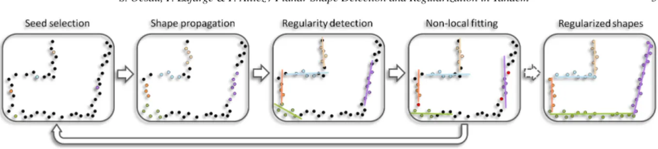
shapes through region growing (Section3). During growing we repeatedly interrupt the shape detection process in or-der to detect non-local relationships between the shapes that have been detected so far (Section4). The shapes are regu-larized according to these relationships (Section5), and we iterate until complete detection, i.e., until no more points can be assigned. We provide below a pseudo-code of the Alg.1, and Figure2depicts the overall process.
Algorithm 1 Interleaved detection and regularization generate octree
compute kNN c← leafCells repeat
for all cido in parallel
if NOT hasActiveShape (ci) then
findSeed (ci)
end if
growShapes (ci)
end
g← detectRelations
for all groups of shapes gido in parallel
regularization (gi)
adjustCoplanarity (gi)
end
until no new points assigned
Our motivation for such methodology stems from the fol-lowing observation: Knowledge about dominant directions and non-local relationships between a preliminary set of shapes detected from the input data can aid further detec-tion by guidance. The key is thus to derive such reladetec-tionships from the input data early during the detection process, which is possible only if a sufficient number of shapes are already detected. To provide many shape hypotheses early in the de-tection process and to achieve short running times, we detect a high number of independent shapes in parallel. As parallel methods are efficient only when the amount of synchronized access is minimized, we favor a region growing approach that operates locally by expanding the borders of a connected region. In addition, region growing is an incremental pro-cess, providing knowledge about a primitive shape before it has been entirely detected. Note that after each region grow-ing performed in parallel, each shape is refitted to its asso-ciated points to improve data fidelity. The regularities are detected and turned into a graph of relationships between shapes which represent a set of regularity hypotheses. To re-inforce the detected relationships between shapes we simu-late non-local fitting from these hypotheses, and verify the fidelity of the regularized shapes with respect to the associ-ated points. Albeit outliers must be accepted when seeking for outlier robustness, the shape is not regularized and we
rollback to the former detected shape when a too large frac-tion of the points does not fit well. Such rollback provides us with resilience to bad decisions taken in the early steps of the detection process, and to imperfect choices of seed points. Detaching points that are no longer faithful to the shape provides guaranteed data fidelity, i.e., maximum Eu-clidean distance between input points and extracted shapes.
3. Shape Detection
Primitive shapes are detected through region growing. A shape is represented as a set of points and associated fitting plane. Growing is achieved either by adding neighbor points to shapes in parallel, or by hierarchical pairwise merging of shapes when they are detected as being both adjacent during growing, and coplanar during the regularity detection step. However, to avoid the need for synchronized access, we re-strict the growing of each shape to its cell. As we deal with unstructured point clouds and growing in parallel on GPU, several key ingredients need to be defined: a local neighbor-hood, an error metric to decide propagation and the criteria to best select seed points.
Local neighborhood. Unstructured point clouds do not provide neighborhood information required for region grow-ing. A typical solution is the range search to determine the neighbors, e.g., in a spherical neighborhood. However, for point clouds acquired by laser scanners this is impractical due to highly variable density and anisotropy. We rely in-stead upon a K-Nearest Neighbor (kNN) graph data struc-ture to determine point-neighborhood during growing, as it better adapts to variable point density.
Growing error metric. The error metric used to decide whether a neighbor point well fits a shape for growing in-volves two error tolerance parameters: ε defines the maxi-mum Euclidean distance between a point and the plane of a shape, and α defines the maximum angle deviation between the normal of a point and the normal of the plane of a shape. The shape propagation is illustrated by Figure4.
Seed point selection. The choice of seed points to initial-ize parallel region growing has some impact on the qual-ity of results and running times. We define two criteria: pla-narity of neighborhood and minimal distance to the cell cen-ter. For planarity we favor seeding points with a high num-ber of unassigned neighbors (out of the kNN) that well fit a plane, according to the error metric. Neighbors already as-signed to another shape are not considered for fitting. Such planarity criterion indicates the presence of a planar struc-ture, favorable to growing, but our experiments showed that seeding closer to cell centers avoids considering already as-signed neighbor points and hence supports faster growing. However, we give a strict priority to the planarity criterion and use the distance to the cell center as a second priority as the first does usually not lead to a unique choice. Seed points
Figure 2: Interleaved detection and regularization. Our method operates a concurrent region growing process for detecting shapes, depicted by different colored points in the first step. The region growing process is interleaved with a regularization of the shapes. Relationships between shapes are detected from locally fitted planes and reinforced by non-local fitting of the shapes during detection. Fidelity to the input points is verified by checking the regularized shape against the associated points. A small number of outliers is acceptable to allow for resilience to outliers and noise (see green shape). A major deviation of a regularized shape from the input points triggers a fallback to local fitting for further propagation (see purple shape).
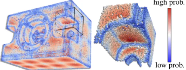
are repeatedly selected during the detection process, when no shape can grow further in this cell and there are unas-signed points left. Region growing is restricted to operate within one cell of the space partitioning. With one exception however: When the growing shape hits the boundary of the cell, neighbor points from other cells well fitting the shape are marked as best candidate seed points. Figure5depicts a point set with probability function to be selected as seed points.
Hierarchical pairwise merging. The space partitioning is created during preprocessing without knowledge about the structure of the input point cloud. A planar part may have been split into several cells and hence detected in parallel
1. iteration 14% coverage 2. 52% 3. 65% 7. 88%
Figure 3: Iterations. After iteration 1, more than 1.000 shapes are detected in parallel. After iteration 2, 52% of the input points are assigned to 250 larger shapes. After iter-ation 3, 65% of the input points are assigned to 140 even larger shapes. Upon termination (iteration 7), 86 shapes cover 88% of the input points.
Figure 4: Growing error metric. We grow a shape by adding neighbor points, indicated by a gray circle, of the bound-ary points, depicted as yellow. Each neighbor point within the ε-domain around the shape and a small deviation of the normal to the shape normal is associated to the shape. Two points in the neighborhood, marked as green, satisfy this condition. Two other points, depicted as red, fail the condi-tion by a major deviacondi-tion of the normal or a posicondi-tion outside of the ε-domain. Growing is carried out for the neighbor-hood of the two newly associated points, depicted in yellow in the right picture.
in different cells. Two shapes belonging to the same planar surface are detected as being coplanar during the regularity detection step. They are merged into one shape if they are also detected as being adjacent during growing, see Fig.3. Finalization. A shape is considered to be finalized, i.e., not active, if no more neighbor points can be assigned.
4. Regularity Detection
We consider three types of relationships between shapes: parallel, orthogonal and coplanar. Given a configuration of shapes with associated points the regularity detection step constructs a conflict-free graph of relationships. The nodes of this graph represent groups of parallel shapes that are con-nected to groups of orthogonal shapes. This graph is later
used during the regularization step. Parallel shapes are de-tected via mean shift clustering in the Gauss normal map, while orthogonal relationships between clusters of parallel shapes are greedily added in a second step by comparing their mean directions. Coplanarity relationships are detected later and are not represented through the graph. For each reg-ularity detection step the relationships are re-learned from all shapes and the graph is rebuilt entirely.
Parallelism. We first generate clusters of parallel shapes. A parameter β is used to specify the tolerance angle deviation between two shape normals. A simple pairwise comparison is not sufficient as a constellation of three shapes a, b and c may already conflict if |na· nb| ≥ cos β and |nb· nc| ≥ cos β,
but |na· nc| < cos β. Instead we perform a Gauss-map
clus-tering. Each shape is projected onto the unit sphere by its normal and assigned a weight equal to the number of asso-ciated points. As we consider unoriented normals we also consider the mirrored point on the sphere. The peaks are ex-tracted via mean-shift, restricted to one hemisphere, using a Gaussian kernel with σ = β. All shapes within one peak are considered to be parallel facing in the direction of the peak. Orthogonality. In a next step we add orthogonal relation-ships to the graph, by pairwise comparison of the directions of the parallel clusters. Initially we put all clusters into a pool, then perform a greedy selection, starting by remov-ing the cluster with highest number of points, as this ter is expected to provide the highest confidence. Two clus-ters c1and c2are considered to be orthogonal if |nc1· nc2| < cos (π
2− β). All clusters orthogonal to the current one, are
connected to the current one by an orthogonal edge and re-moved from the pool. We repeat this greedy selection by choosing the next cluster with the highest number of points remaining in the pool. Upon termination the graph consist-ing of several disconnected subgraphs.
Given an indoor scan of a Manhattan world environment for high prob.
low prob. Figure 5: Seed point selection. The point set of a mechan-ical part is colored by the probability of a point to be cho-sen as a seed point for the region growing process. Points close to sharp features are assigned a low probability as their neighborhood is non-planar. On flat parts of the sur-face points closer to the cell center of the space decompo-sition are favored as they allow for a faster expansion not being bounded by the borders of the cell.
instance, all shapes of the structures are ideally contained in one subgraph. The center-node of the subgraph represents the largest number of points associated to parallel shapes, in this case probably the direction of floor and ceiling. Two nodes are connected to the center-node, each containing the shapes of one wall direction.
Coplanarity. Coplanarity relationships are detected only after reorienting the shapes in the regularization step (Sec-tion5), as shapes detected to be approximately parallel have already been regularized to be exactly parallel. For each group of parallel shapes we perform a clustering based on the distance between the planes. More specifically, the (clus-tered) shapes are projected onto points on the line defined by their shared normal through the origin. Each shape is weighted by the number of points associated to the shape. We then cluster the shapes through mean-shift applied to these projections, through a Gaussian kernel parameterized with σ = ε.
5. Regularization
Provided a set of shapes with associated points and a graph of relationships, we regularize the shapes by performing constrained plane re-fitting where constraints are in accor-dance to the graph. Plane fitting is performed through prin-cipal component analysis (PCA), extended to fit multiples planes with a fixed relative orientation.
The best least squares fitting plane to a set of points of a shape Sipasses through the center of mass µi, and its normal
is aligned to the vector with minimal variance of the points. PCA provides an orthogonal basis aligned to the principal variation of the data by extracting the eigenvectors of the co-variance matrix covi.
The eigenvectors of covi denote the orthogonal directions
of variation and the corresponding eigenvalues quantify the amount of variation. Only the eigenvector ~x of the smallest eigenvalue needs to be determined as this corresponds to the orientation of the plane. As we perform iterative re-fitting with reliable initial guesses and perform all computations in parallel on GPU we find it more efficient to compute the smallest eigenvalue through the power iteration method ap-plied to the inverted covariance matrix.
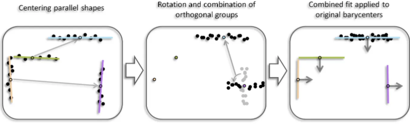
We extend the common plane least squares fitting to the fitting of clusters of planes with a fixed relative orienta-tion (either parallel or orthogonal) by combining the co-variances matrices into one a single matrix. The covariance matrix measures the variance relative to the centered data and is therefore translation invariant. For a cluster of parallel shapes the covariance matrices coviof each shape’s point set
are thus simply added. For clusters of parallel shapes that are mutually orthogonal we choose as “master” shape the one with largest number of points and all clusters of orthogonal shapes connected in the graph are rotated around their center of mass to match the master shape. Rotation Riis specified
Figure 6: Constrained non-local refitting. The orientation of regularized shapes is defined in one fitting step to guarantee exact parallelism and orthogonality between regular shapes. The points of parallel shapes are translated by moving the center of mass into a single location (left). Points of mutually orthogonal shape clusters are combined by rotating the points by π 2
around the cross product of the mean direction of each group (middle). The normal of the least-squares fitting plane is the best fit orientation for the parallel shapes and the inverse rotated normal for the orthogonal groups respectively (right).
by using the cross-product between the normals of Siand of
the master shape as axis andπ
2 as rotation angle. We weight
the influence of each set of points by multiplying their co-variance matrix by a weight set to the number of points:
cov =
∑
i
(|Si| · covi) (1)
The regularized planes of the shapes are then given by the backward transformed direction and the individual barycen-ter µi or the mean barycenter for coplanar shapes, see Fig.
6:
(R>i~x)p − (R>i~x)µi = 0 (2)
6. Implementation Details
Our algorithm is implemented in C++ and in CUDA using compute capability 1.1. We use the CGAL library for fast normal estimation when not provided with the input points. Execution of an algorithm on GPU requires a structuring into single kernels, i.e. functions, that are called from CPU and executed in parallel by blocks of threads. Further information about CUDA and GPU architecture can be found in the CUDA documentation.
During the preprocessing we generate an octree and com-pute the approximate K Nearest Neighbors (akNN) for each input point. We choose an octree for space partitioning as it provides a decomposition into compact cells and can be implemented very efficiently on the GPU. The 3D morton code is a space filling curve, that follows a depth-first traversal of an octree. We calculate the arc-length of each point on the curve and sort the points by radix sort. Karras et al.[Kar12] recently published an efficient method following this approach. A precision of 30 bits for the morton code, which correspond to a maximal octree depth of 10, proved to be sufficient in our experiments.
To compute the akNN we rely on the octree data structure
created to distribute the work with a fine partitioning. We identified that maintaining the buffers of the k nearest neighbors, i.e., indices and distance, for each point during calculation is expensive. Resorting the buffer is minimized if the nearest neighbors are considered first. Therefore we start by pairwise comparison of points within an octree leaf cell first. In the next step neighboring octree cells are identified by traversing the octree and only points close to the boundary of neighboring cells are further processed. We restrict the search for the n nearest neighbors for each octree cell to its adjacent cells.
The main information is kept in three data structures in global memory during processing. First, we define a shape structure data type specific to one octree cell containing the local fit and regularized plane equation, mean and covari-ance values for fitting as well as affiliation with a group of parallel shapes and merged shapes. As dynamic allocation of memory is costly or not available on older GPUs, we preallocate an array of memory and provide access via atomic increment of an index to next free structure. New shape structures are only instantiated during the findSeed step.
The second data structure stores the leaf cells of the octree. The octree structure itself is discarded as only the leaf cells are required to access the points within the range of those cells. Additionally, the cell data structure is used to propagate seed points across cells (see3). A ring buffer with accessed via atomic operations is used for synchronized access.
The last data structure is the shape index, a map from a point to the associated shape structure.
The findSeed step translates to a single kernel launch with a number of blocks equal to the number of octree leaf cells. In case of no active shape inside a cell a new shape is instantiated by taking the next propagated seed point from
the ring buffer in the cell structure or otherwise by searching the points within the cell. In case of searching the points in the range of a cell are divided among the threads of the block and the most suitable seed point for each thread is stored in shared memory. A subsequent reduction retrieves the chosen seed point.
Algorithm 2 growShapes - kernel c← cells[blockIdx]
f← c. f irstIndex l← c.lastIndex
for all s ← active shapes do
map bu f f er[i] ← shapeIndex[i], for i ∈ [ f , l] for n iterations do
for all i ∈ [ f , l] do in parallel if bu f f er[i] = to be visited then
if metric(s, pi, ni) then set kNN of piin buffer end if end if end end for sum reduce µs
sum reduce covs
refit(s, µs, covs)
end for
The growShapes step also translates to a single kernel launch and instantiates one block per octree leaf cell, see Alg.2. Within a block all active shapes of one cell are grown subsequently by first performing a coalesced map operation from the shape index in the range of the cell into a separate buffer used for growing. The value in the buffer indicates the state of a point: not visited, to be visited, associated or rejected. In case of regularized shapes, points are filtered that do no longer satisfy the error metric, see Fig.4. A map was chosen for tracking the recently added points instead of a list to avoid synchronization mechanisms.
The growing is performed via a scatter operation of the buffer into itself. The metric is evaluated for points marked as to be visited are tested, and the kNN are marked as to be visitedif not yet visited. Keeping track of the highest and lowest index of to be visited allows to restrict the mapping operation in each iteration to this interval. The shape index is updated with the points added to the shape. The state of the shape is set to inactive if no additional points could be found during growing.
Refitting the shape to the associated points is performed by a sum reduction of the positions to retrieve the mean of the points. A second reduction yields the covariance matrix. The inverse power iteration to retrieve the eigen-vector is performed by a single thread in each block, but
is performed quickly as it requires only little memory access.
Algorithm 3 regularization sum scan for Gauss map creation repeat
peaks← mean shift in parallel filter peaks
shape groups←remove shapes from Gauss map
until Gauss map is empty
master shape groups← construct relationship graph for all s ← active shapes do in parallel
sum scan covs
end
for all master shape groups do in parallel constrained fitting
end
for all shapes do in parallel verify alignment
end
The regularization step consists of several kernels, see Alg.3. At first the Gauss map clustering is performed to identify parallel and orthogonal groups. We once generate a set of normals covering the hemisphere roughly uniformly and thereby defining bins for the clustering. The discretiza-tion is chosen as the regularizadiscretiza-tion angle tolerance β, but not lower than 10◦. The first kernel counts the shapes that fall into each bin. A sum scan is used to identify the memory ad-dresses to reorder the shapes in a buffer such that the shapes of each bin are linear in memory. The mean shift clustering is performed in a loop. A kernel is launched for each non-empty bin using the average normal in this bin as the starting value. Grouping the shapes by bins allows to quickly reject all but few bins for mean shift and to copy the relevant shape structures into shared memory. We filter close-by peaks and remove clustered shapes from the buffer. The association to a shape group is set as a variable in the shape structure The mean-shift is restarted with the remaining non-empty bins. Typically only a few iterations are required.
The relationship graph is constructed by a kernel launched as a single block as the number of groups is usually very low, up to 22 in our experiments.
To perform the constrained fitting the covariance matrices of shape groups that are mapped onto another shape group have to be rotated. A kernel is launched with one block per shape that performs a sum reduction of the rotated points if required and writes the covariance matrix into the shape structure. The constrained fitting is performed in a single kernel call that performs a sum reduction, see Eqn.1, and
Outliers/Noise
Figure 7: Robustness. We sampled the model uniformly and tested our method while increasingly adding outliers and Gaussian noise. With an increasing amount of noise and out-liers small shapes are more difficult to detect. The closeup depicts a section with narrow windows that is affected by the increase of noise. However, the coarse structures are still de-tected for a strong amount of defects, depicted by the full set of detected shapes in the upper row.
performs the refit as in growShapes. As the number of mas-ter shape groups is known from relationship construction, the kernel is launched with one block for each.
The coplanarity adjustment is performed in a single kernel, one block launched per shape group. We map the shapes of each group into shared memory, as the only required infor-mation are the projected position on the direction, the num-ber of points and the index of the shape structure in the global array. A mean shift is performed in each thread. We chose the starting position for each thread by uniformly di-viding the range of projected positions.
The verification of the realigned shapes is formulated as a mapping operation, where all points of a shape are detached in the shape index, that do no longer satisfy the metric, see Fig.4.
7. Experiments
Benchmark. Surface reconstruction and shape detection have common topics of research, hence a set of common criteria for evaluation have been established [BLN∗13]. Depending on the type of input data and defects such as missing data or outliers, some criteria such as the Hausdorff distance may not be relevant. To measure geometric fidelity we choose the mean distance of a detected shape to its associated points. The coverage, i.e., percentage of points assigned to primitive shapes, is used as indicator for com-pleteness of the detection. The running times listed in Table
1include all preprocessing steps such as octree generation and kNN. For evaluation we used a MacBook Pro laptop with Core i7 4850HQ and a GeForce GT 750M graphics card.
Evaluating the regularity of a set of primitive shapes
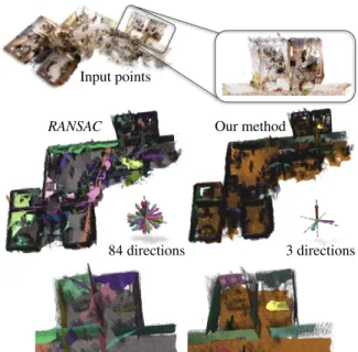
84 directions 3 directions
Input points
RANSAC Our method
Figure 8: Kinect. This Manhattan world scene has been acquired by a mobile robot using Kinect sensors and reg-istered into a single point set. Schnabel’s method detects many shapes but they are not very well aligned due to the high amount of noise and clutter and imprecise registration. Our methods identifies the main directions of the Manhattan world and aligns the shapes with those directions during de-tection. This allows for compensation of the imprecise regis-tration, see lower image row for comparison with Schnabel’s method.
is still quite unexplored. We measure the complexity of a set of planar shapes by the degrees of freedom of the corresponding planes. High complexity refers to low regu-larity and vice-versa. A plane has three degrees of freedom: two for the orientation and one for the signed distance to the origin. For a group of parallel shapes we count only two degrees of freedom for orientation. For two or more pairwise orthogonal set of shapes we consider three degrees of freedom in total for the orientation. Coplanar shapes count for one.
We compare our method against three other methods to evaluate the shape detection performance and the regularity: a region growing method (RegGrow) for detecting planar shapes in unstructured point data [LM12], the efficient RANSAC-based shape detection method (RANSAC) pro-posed by Schnabel et al. [SWK07], and GlobFit [LWC∗11], an iterative regularization method relying upon the afore-mentioned RANSAC method. For rigorous comparison we set the parameters of these methods to provide results with similar mean errors and minimum number of points per shape. While RANSAC and GlobFit can handle other types of shapes we restrict the methods to planar shapes for
large
small
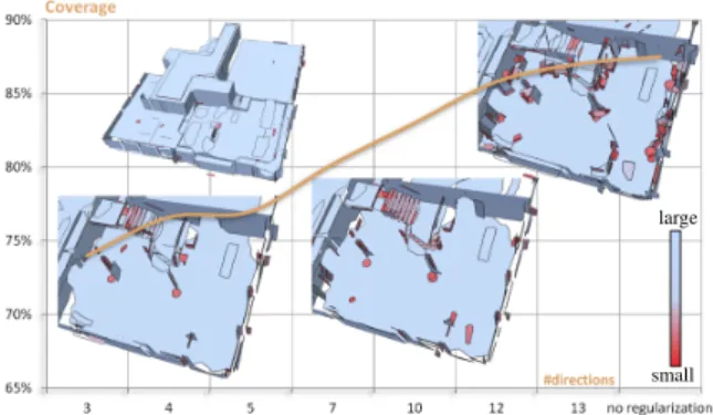
Figure 9: Regularity vs. coverage. Favoring strong regular-ity may come at the cost of coverage. We applied our method to the LIDAR data set ’Euler’ with different parameters. Col-ored scale refers to the shape area. The full reconstruction with low regularity is shown in the upper left. A high amount of clutter in the entrance hall can be seen on the upper right closeup with a low regularity, i.e. 388 different directions. The two closeups in the lower figure show the variation in detection of irregular shapes, clutter, while favoring a higher regularity, i.e., 5 and 10 different directions. Many small shapes on clutter are detected while the shapes on structural parts remain mostly untouched.
comparison.
We choose several data sets for evaluation, ranging from architectural scenes acquired via laser scanners and Kinect sensors to a point set acquired by Multi-View Stereo (MVS) using the approach from Vu et. al [VKLP09]. The Kinect point set covers an indoor Manhattan world scene [ GM-RFM14]. On defect-laden inputs our experiments show that the interleaved regularization improves the shape detection step through detected relationships, see Figure8.
The RANSAC method shows a comparatively low compu-tation time compared to RegGrow, but is significantly slower than our GPU-based algorithm. While the coverage of the data is similar to ours, RANSAC does not perform any regu-larization and therefore exhibits low regularity. The coverage of RANSAC is similar to the one produced by our method, al-beit the process devised to ensure connected components is not adaptive to variable point density and has impact on the running times. Choosing a small tolerance for connectivity leads to a separate detection of details in densely sampled areas and to absence of detection in sparse areas. A high tol-erance for connectivity leads to loss of details in dense areas, but yields reconstruction in sparse areas (Figure10). The RegGrow method achieves a higher coverage in almost all experiments compared to the two other methods, but the
number of detected primitives is higher while all methods are set to use the same minimal number of points per shape. The comparison with our region growing mechanism shows, that in some cases the regularity of shapes may come at the cost of coverage, see Fig.9.
For evaluating GlobFit we used the implementation provided by the authors, and rely upon the output of RANSAC as in the original publication. It can optimize for wider range of rela-tionships, but is both memory- and compute-intensive. This renders the method unsuitable for datasets at the scale of ur-ban scenes, and we could compare on a single data set due to excess of memory consumptions. On the Kinect data set the regularization yields high regularity by enforcing a Manhat-tan world providing a similar result to our method.
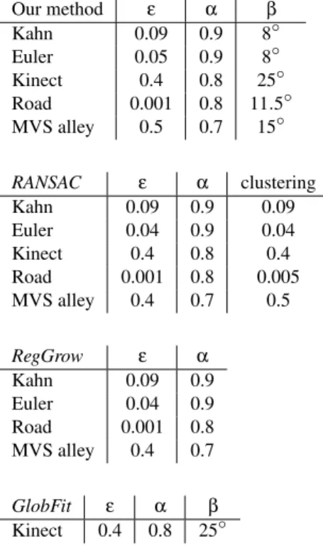
The parameters used in our experiments are listed in Table
2.
Robustness. To evaluate the robustness of our method we manually designed a model of a house in Trimble Sketchup and generated a defect-laden point set. Such designed model provides us with a ground truth: we can distinguish between points sampled from a shape and added outliers, and thus correctly measure the coverage and fidelity to the ground truth, see Figure7.
The constantly recurring detection and reinforcement of non-local regularities makes the method resilient against outliers, noise and sparse sampling. By jointly fitting par-allel shapes the accuracy in sparsely sampled noisy areas is reinforced by parallel shapes from densely sampled areas, see Fig.8. The region-growing method inherently provides to some extend outlier robustness due to its local propagation mechanism.
Parameters. The algorithm requires selecting few parame-ters: ε, the Euclidean tolerance error distance between shape and input points, α, the normal tolerance deviation between shape and input samples, and the minimum number of points per shape are common among shape detection methods. β is the maximum angle deviation used to consider two planes as parallel during the detection of regularities.
The chosen cell size for octree creation determines the num-ber of generated leaf cells and therefore the degree of paral-lelism in execution. Per iteration of the method at most one seed point is chosen per cell and therefore at most one shape per cell is detected. A separation into few large cells allows further expansion of single shapes, but requires more iter-ations for detecting all shapes and leads to inefficient load balancing. Many small cells, however, lead to better load balancing, but might add some overhead due to the increase of shapes for regularization and fitting. A graph evaluating the impact on cell size on performance is shown in Fig.11. For point sets mainly consisting of large planar shapes, e.g. architecture captured by a laser scanner, a high cell size leads to a higher performance. An upper cell size limit is imposed by the hardware specification of the GPU. Choosing a cell
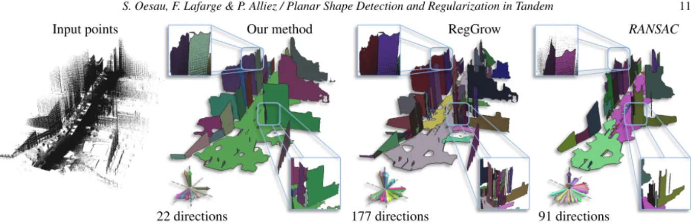
Input points Our method RegGrow RANSAC
22 directions 177 directions 91 directions
Figure 10: Road. This data set was acquired from a car moving along a street. The point density strongly varies from the road towards the top of the buildings. Our method (mid left) and the RegGrow method (mid right) exhibit resilience against varying point density and are able to detect details close to the road as well as shapes in sparse areas. The RANSAC method does not adapt well to the sparse sampling and is not able to detect the upper parts of the buildings, see excerpts in upper part. This leads to a lower coverage79.3% vs. 87.8% (our method) and 88, 7% (RegGrow), see Table1. The RegGrow method tends to a higher number of primitives compared to the other methods, shown in the lower excerpt showing a curved part of a building. The result of our method shows a stronger regularity compared to RegGrow.
data sets methods evaluation criteria output complexity
mean error coverage time complexity #shapes #dirs #planes
Our method 0.045 72,0% 8.7s 0.33 200 12 179 Kahn RANSAC 0.041 72,4% 34.9s 0.98 200 195 200 (5.2M pts, Fig.1) RegGrow 0.044 76,6% 348s 0.94 295 272 290 Our method 0.014 81,0% 5.1s 0.37 133 14 120 Euler RANSAC 0.011 81,8% 26,2s 0.99 232 228 232 (3.9M pts, Fig.9) RegGrow 0.012 87,1% 379,1s 0.97 284 273 284 Our method 0.22 43,6% 2.2s 0.30 47 3 39 Kinect RANSAC 0.26 84,8% 12.6s 1.0 84 84 84 (0.3M pts, Fig.8) Globfit 0.24 50,5% 185s 0.34 48 3 46 Our method 1.6 87,8% 5.2s 0.49 73 22 63 Road RANSAC 1.6 79,3% 28.3s 1.0 91 91 91 ( 1.4M pts, Fig.10) RegGrow 1.52 88,7% 102s 0.96 185 177 181 Our method 0.031 83,3% 3.2s 0.42 69 11 67 MVS alley RANSAC 0.028 82,2% 8.5s 1.0 55 55 55 ( 1.1M pts) RegGrow 0.028 83,2% 29s 0.99 133 132 133
Table 1: Benchmark. The Kahn and Euler data sets represent buildings acquired by a laser scanner. The Kinect data set shows a small indoor scene of several registered Kinect scans. The Road data set shows a urban scene recorded by a laser scanner mounted on a car. A multi-view stereo data set, MVS alley, was used to test the methods on another kind of data featuring stronger noise, irregular and incomplete sampling.
Time (ms)
Cell size (points)
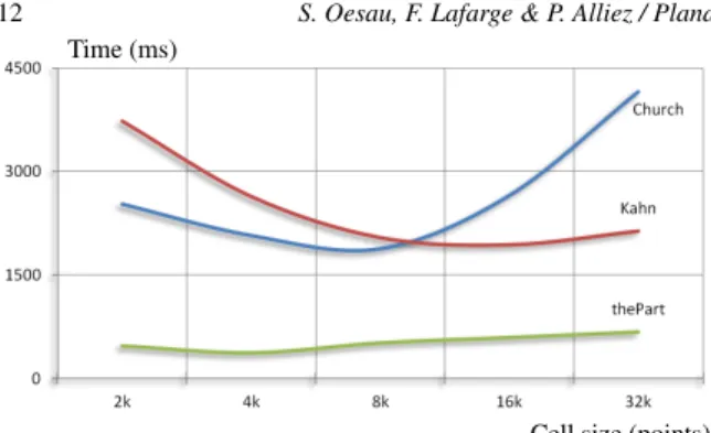
Figure 11: Octree parameters. We depict the impact of the chosen cell size of the octree upon the running time. The Kahn data set is shown in Fig.1, ’church’ in Fig.3 and ’thePart’ in Fig.5. The Kahn data set has been acquired by a laser scanner and features a high point density with low noise. A larger cell size enables fast shape growing not lim-ited by the space decomposition. The church data set instead exhibits higher noise, lower point density and less points per shape. A smaller cell size enables detecting all shapes with fewer iterations, as only one shape per cell and iteration can be detected.
size leading to fewer cells than the GPU can handle in par-allel will not use the full capacity of the GPU. Otherwise, for more detailed geometry a smaller cell size is preferable. However, in our experiments we found a cell size of 8k suit-able in most cases.
Region growing iterations between regularization
Figure 12: Synergy between regularization and detection. We evaluate the mutual benefit between detection and reg-ularization by varying the alternating frequency. A progres-sive detection and regularization yields higher detection rate and regularity, at the cost of increased computational time due to additional regularization, compared to a less pro-gressive or even purely sequential process. A highly frequent alternation, however, provides no additional gain for the ad-ditional invested computations.
The chosen number k of nearest neighbors impacts the propagation speed of shapes and the ability to handle
anisotropic data. However, the kNN are stored for each in-put sample in memory on GPU and imposes a restriction to the maximum number of points that can be processed at once. In our implementation for each input sample the po-sition, the normal and two integer flags are stored on GPU. This leads to a memory consumption of 32 Bytes + k × 4 Bytes per point. For a common choice such as k = 20 each sample point consumes 112 Bytes. For a GPU with 1GB of memory the maximum number of points to process at once is around 8-9M considering a few other memory structures (GPUs with 12GB memory are available but not yet routine). Synergy of regularization and detection. A distinctive property of our algorithm is the interleaved detection and regularization. We evaluate our method with respect to se-quential approaches by varying the frequency between de-tection, i.e. region growing, and regularization. We use as input our sampled ground truth model with added noise and outliers (resp. 0.2% and 20%) and measure both coverage (in percent with respect to the sampled points) and regular-ity, see Fig.12. This experiment shows that regularization provides a guidance during detection leading to a higher fi-delity to the sampled points. Notice that a high frequency yields no further benefit and increase computational times. A very low frequency or even a purely sequential approach leads to shapes with large spatial extend. The regularization potential of these large shapes is limited as, in general, a change in orientation implies a large deviation from its as-signed points.
Figure 13: Detection on curved shapes. This mechanical part contains several cylindrical surface parts at different scale as well as planar parts. The regularization of planar shapes on curved surfaces may lead to the detection of ir-regular interfaces between shapes or over-segmentation, de-picted in the lower left close-up. Some small shapes approxi-mating the cylindrical parts are aligned to the larger planar shapes (right). Note however that the regularization of the larger planar parts is not contaminated by those cylindrical parts.
Limitations. While providing fast detection and alignment of planar structures our method is not designed for the recon-struction of free-form shapes. Our algorithm approximates curved surfaces by planar patches. However, due to the con-finement of the region growing within one cell the orienta-tion of the space partiorienta-tioning is likely to impact the detected
Figure 14: Stability on curved shapes. The fandisk model exhibits surface parts with different curvature. Our method approximates curved areas by smaller planar shapes of dif-ferent size. A small variation of the ε parameter, e.g. 0.1 (left) and0.095 (right), might lead to larger variation in the re-sults.
shapes on curved parts, see Fig.13. Our method might lack stability with respect to the ε parameter on curved shapes, see Fig.14.
Processing data on the GPU provides the benefit of highly parallelized processing. However, it comes with a memory restriction limiting the size of the data sets that can be pro-cessed. This is partially due to the kNN for the shape propa-gation as k indices must be stored for each input sample.
8. Conclusion
We presented a method for detecting and regularizing planar primitive shapes from unorganized point clouds acquired on man-made physical scenes. A novel aspect of our method consists in interleaving shape detection and regularization so as to make the two processes mutually cooperate. Such approach is shown to improve detection and robustness, in particular when dealing with defect-laden data. Another con-tribution is to design all data structures and algorithm com-ponents with an eye on constraints of modern GPU architec-tures. Our experiments on a variety of point clouds demon-strate the added value of our approach in terms of efficiency, detection quality and regularity. The main parameters of our algorithms provides us with a means to trade coverage for regularity.
In future work we will investigate the use of compact data structures on GPU to improve scalability. We also wish to understand the hierarchical relationships between shapes in order to detect and utilize more structure from the input raw data.
9. Acknowledgments
The authors wish to thank Airbus - Defense and Space for funding this work. Pierre Alliez is supported by an ERC Starting Grant "Robust Geometry Processing" (257474).
Our method ε α β Kahn 0.09 0.9 8◦ Euler 0.05 0.9 8◦ Kinect 0.4 0.8 25◦ Road 0.001 0.8 11.5◦ MVS alley 0.5 0.7 15◦ RANSAC ε α clustering Kahn 0.09 0.9 0.09 Euler 0.04 0.9 0.04 Kinect 0.4 0.8 0.4 Road 0.001 0.8 0.005 MVS alley 0.4 0.7 0.5 RegGrow ε α Kahn 0.09 0.9 Euler 0.04 0.9 Road 0.001 0.8 MVS alley 0.4 0.7 GlobFit ε α β Kinect 0.4 0.8 25◦
Table 2: Parameters used in experiments. All methods use ε as the maximum tolerance Euclidean distance between a point and a shape. α denotes the normal deviation threshold α ≤ npoint· nshape. β denotes the normal tolerance between
shapes to be considered as parallel during regularization. RANSAC requires one additional parameter for clustering neighbored points by distance. Globfit operates on top of RANSAC hence uses the same parameters for detection. Pa-rameter ε is used for coplanarity alignment in Globfit. The minimum number of points for all methods is set to 500 for the Kahn, Euler and Road data sets, 200 for Kinect and 100 for MVS alley.
References
[ASF∗13] ARIKANM., SCHWARZLERM., FLORYS., WIMMER
M., MAIERHOFERS.: O-snap: Optimization-based snapping for modeling architecture. TOG 32, 1 (2013).1
[BCM05] BUADESA., COLLB., MORELJ. M.: A non-local algorithm for image denoising. In CVPR (2005), vol. 2.3
[BELN11] BORRMANN D., ELSEBERG J., LINGEMANN K., NÜCHTERA.: The 3D Hough Transform for plane detection in point clouds: A review and a new accumulator design. 3D Research 2, 2 (2011).2
[BLN∗13] BERGERM., LEVINEJ. A., NONATOL. G., TAUBIN
G., SILVAC. T.: A benchmark for surface reconstruction. TOG 32, 2 (2013).9
[BM12] BOULCHA., MARLETR.: Fast and robust normal esti-mation for point clouds with sharp features. CGF 31, 5 (2012).
2
[Che95] CHENGY.: Mean shift, mode seeking, and clustering. PAMI 17, 8 (1995).2
[CLP10] CHAUVE A.-L., LABATUT P., PONS J.-P.: Robust piecewise-planar 3D reconstruction and completion from large-scale unstructured point data. In CVPR (2010).2
[Dav05] DAVIESE. R.: Computer and Machine Vision: Theory, Algorithms, Practicalities. Morgan Kaufmann Publishers Inc., 2005.2
[FB81] FISCHLERM. A., BOLLESR. C.: Random sample con-sensus: A paradigm for model fitting with applications to im-age analysis and automated cartography. Communications of the ACM 24, 6 (1981).2
[GMRFM14] GOKHOOL T., MEILLAND M., RIVES P., FERNÁNDEZ-MORALE.: A dense map building approach from spherical rgbd images. In VISAPP (3) (2014).10
[HB12] HOLZD., BEHNKES.: Fast range image segmentation and smoothing using approximate surface reconstruction and re-gion growing. In IAS (2) (2012), vol. 194.3
[Hou62] HOUGHP. V. C.: A method and means for recognizing complex patterns, 1962. U.S. Patent No. 3,069,654.2
[KAJS11] KOPPULAH., ANANDA., JOACHIMS T., SAXENA
A.: Semantic labeling of 3d point clouds for indoor scenes. In NIPS(2011).1
[Kar12] KARRAST.: Maximizing parallelism in the construction of bvhs, octrees, and k-d trees. In Proceedings of the EURO-GRAPHICS Conference on High Performance Graphics 2012, Paris, France, June 25-27, 2012(2012), pp. 33–37.7
[LA13] LAFARGE F., ALLIEZ P.: Surface Reconstruction through Point Set Structuring. CGF 32, 2 (2013).1
[LM12] LAFARGEF., MALLETC.: Creating large-scale city models from 3D-point clouds: a robust approach with hybrid rep-resentation. IJCV 99, 1 (2012).9
[LWC∗11] LI Y., WU X., CHRYSANTHOU Y., SHARF A., COHEN-ORD., MITRAN. J.: Globfit: Consistently fitting prim-itives by discovering global relations. TOG 30, 4 (2011).3,9
[MWA∗13] MUSIALSKIP., WONKAP., ALIAGAD. G., WIM
-MERM.,VANGOOLL., PURGATHOFERW.: A Survey of Urban Reconstruction. CGF 32, 6 (2013).1
[PCYS12] PHAMT.-T., CHINT.-J., YUJ., SUTERD.: The ran-dom cluster model for robust geometric fitting. In CVPR (2012).
2
[QZN14] QIUR., ZHOUQ.-Y., NEUMANNU.: Pipe-run extrac-tion and reconstrucextrac-tion from point clouds. In ECCV (2014).2
[RvDHV06] RABBANIT.,VANDENHEUVELF., VOSSELMAN
G.: Segmentation of point clouds using smoothness constraint. ISPRS 36, 5 (2006).3
[SDK09] SCHNABELR., DEGENERP., KLEINR.: Completion and reconstruction with primitive shapes. CGF 28, 2 (2009).1
[SHFH11] SHEN C.-H., HUANG S.-S., FU H., HU S.-M.: Adaptive partitioning of urban facades. TOG 30, 6 (2011).2
[SSS∗08] SINHAS., STEEDLY D., SZELISKIR., AGRAWALA
M., POLLEFEYSM.: Interactive 3d architectural modeling from unordered photo collections. TOG 27, 5 (2008).1
[SWK07] SCHNABEL R., WAHL R., KLEIN R.: Efficient RANSAC for point-cloud shape detection. CGF 26, 2 (2007).
2,3,9
[VGSR04] VOSSELMANG., GORTEB., SITHOLEG., RABBANI
T.: Recognising structure in laser scanner point clouds. ISPRS 46, 8 (2004).1
[VKLP09] VUH.-H., KERIVENR., LABATUTP., PONSJ.-P.: Towards high-resolution large-scale multi-view stereo. In CVPR (Miami, Jun 2009).10
[XRT12] XIAOJ., RUSSELLB. C., TORRALBAA.: Localizing 3d cuboids in single-view images. In NIPS (2012).2
[ZN12] ZHOUQ.-Y., NEUMANNU.: 2.5D building modeling by discovering global regularities. In CVPR (2012), IEEE.3