Design and Application of Compliant Quasi-Kinematic Couplings
byMartin L. Culpepper
B. S. Mechanical Engineering Iowa State University, 1995
M. S.
Massachusetts Institute of Technology, 1997
Submitted to the Department of Mechanical Engineering in Partial Fulfillment of the Requirements for the Degree of
Doctor of Philosophy in Mechanical Engineering at the
Massachusetts Institute of Technology
February 2000
© 2000 Massachusetts Institute of Technology
All rights reserved
Signature of Author.,
Certified by ...
.. .. . . . ..
De tm of Mechanical Engineering January 07, 2000
Professor of Mechancial Engineering Th-zi q Sinervisor
Accepted by ...
Professor Am A. zoonin Chairman, Department Committee on Graduate Studies
MASSACHUSETTS INSTITUTE
OF TECHNOLOGY
SE P 2
0 2000
Design and Application of Compliant Quasi-Kinematic Couplings
byMARTIN L. CULPEPPER
Submitted to the Department of Mechanical Engineering on January 07, 2000 in Partial Fulfillment of the Requirements for the Degree of Doctorate of Philosophy in
Mechanical Engineering ABSTRACT
Better precision at lower costs is a major force in design and manufacturing. However, this is becoming increasingly difficult to achieve as the demands of many location applica-tions are surpassing the practical performance limit (- five microns) of low-cost cou-plings. The absence of a means to meet these requirement has motivated the development of the Quasi-Kinematic Coupling (QKC). This thesis covers the theoretical and practical considerations needed to model and design QKCs.
In a QKC, one component is equipped with three spherical protrusions while the other contains three corresponding conical grooves. Whereas Kinematic Couplings rely on six points of contact, the six arcs of contact between the mated protrusions and grooves of QKCs result in a weakly over-constrained coupling, thus the name Quasi-Kinematic. QKCs are capable of sub-micron repeatability, permit sealing contact as needed in casting, and can be economically mass produced.
The design and application of a QKC is demonstrated via a case study on the location of two engine components. Integration of the QKC has improved coupling precision from 5
to 0.7 microns. In addition, this QKC uses 60% fewer precision features, 60% fewer pieces, costs 40% less per engine, and allows feature placement tolerances which are twice as wide as those of the previous dowel-pin-type coupling.
Thesis Supervisor: Prof. Alexander H. Slocum
ACKNOWLEDGMENTS
I would like to thank my wife for putting up with my long hours of work. She is most pre-cious to me. I thank her for all her support, love, and patience.
To my Dad, who taught me perseverance and my mom who taught me patience, I thank them for helping me walk the straight and narrow. I once asked, "Could they have guessed that their rowdy five-year-old "tinkerer" would one day grow up to be an engi-neer?" They replied, "Yes, you had so much practice breaking things, something had to go right for you."
I would also like to thank Professor Alexander Slocum for his help and inspiration. With-out his guidance I would not have achieved this level of success.
To Profs. Hardt, Sarma, Suh, and Trumper I give thanks for advising me on conducting and publishing research. I would also like to thank them for their guidance on preparing for an academic career.
To Profs. Sarma and Anand I give my gratitude for serving as members of my thesis com-mittee. Their advice and critiques were very helpful.
I would also like to thank F. Z. Shaikh, J. Schim, G. Vrsek, R. Tabaczynski, V. B. Shah, Greg Minch, and Kevin Heck for their financial and technical support during this project.
Finally, I would like to thank God, the ultimate designer in the universe. As a fellow designer, I look at this world and wonder how frustrated He must get with us... Thank God for His patience.
TABLE OF CONTENTS 7
TABLE OF CONTENTS
ACKNOWLEDGMENTS . . TABLE OF CONTENTS LIST OF FIGURES . . LIST OF TABLES ... NOMENCLATURE .... . . . 5 7 . . . . 11 . . . . 1 5 . . . . . 17 CHAPTER 1. INTRODUCTION ... 1.1 M otivation . . . . 1.2 Precision Coupling Systems ... 1.3 Thesis Scope and Organization ... 1.4 Types of Passive Mechanical Couplings ... 1.4.1 Elastic Averaging Methods ... 1.4.2 Pinned Joints ... 1.4.3 Kinematic Couplings ... 1.4.4 Compliant Kinematic Couplings ... 1.4.5 Quasi-Kinematic Couplings (QKCs) . . . 1.4.6 Comparison of Mechanical Coupling Types CHAPTER 2. QUASI-KINEMATIC GEOMETRY AND FUNCTION 2.1 Physical Components of QKCs . . . . 2.2 Analytic Components of QKCs . . . . 2.2.1 Joint Coordinate Systems . . . . 2.2.2 Analytic Components of Coupling . . . . 2.2.3 Contact Angle . . . . 2.3 Function of Quasi-Kinematic Couplings . . . . CHAPTER 3. MODELING AND ANALYSIS OF QKCs... 3.1 Modeling of Quasi-Kinematic Couplings . . . . 3.1.1 Kinematic Coupling Solution . . . . 3.1.2 Solving the QKC Over Constraint Problem . . . 3.2 Quasi-Kinematic Coupling Contact Mechanics... . . . . 21 . . . . 2 1 . . . . 2 3 . . . . 25 . . . . 26 . . . . 26 . . . . 27 . . . . 2 8 . . . . 29 . . . . 30 . . . . 3 1 . . . . 33 . . . . 33 . . . . 34 . . . . 35 . . . . 36 . . . . 37 . . . . 38 . . . . 39 . . . . 39 . . . . 39 ... 41 . . . . 423.2.1 Contact Analysis Using a Rotating Coordinate System . . . 42
3.2.2 Relationship Between Surface Stresses and Force Per Unit Length . . 45
3.2.3 Far Field Distance of Approach . . . . 46
3.2.4 Relationship Between fn and dn . . . . 50
3.3 Using the Quasi-Kinematic Coupling Model/Analysis . . . . 51
3.3.1 Quasi-Kinematic Coupling Reaction Forces . . . . 51
3.3.2 Stiffness of QKCs . . . . 54
3.3.3 Limits on the Estimation of QKC Stiffness . . . 54
CHAPTER 4. DESIGN AND MANUFACTURE OF QUASI-KINEMATIC COUPLINGS . 57 4.1 Overview of the Quasi-Kinematic Coupling Design Process . . . 57
4.2 Problem Definition . . . 58
4.2.1 Constraints . . . 59
4.2.2 Functional Requirements . . . . 59
4.2.3 Design Parameters . . . 60
4.3 Geometry Generation . . . 60
4.3.1 Quasi-Kinematic Coupling Gap . . . . 61
4.4 Design Check . . . . 69
4.5 Iteration If Needed . . . . 70
4.6 Design Specific Quasi-Kinematic Coupling Constraints . . . 70
4.6.1 Enhancing QKC Performance Via Moderate Plastic Deformation . . 70
4.6.2 Affects of Localized Plastic Deformation on QKC Performance . . . 76
4.6.3 Load and Displacement Behavior of QKC Joints . . . . 82
4.6.4 Ratio of Contactor to Target Hardness . . . . 83
4.7 Manufacturing of Quasi-Kinematic Coupling Elements . . . . 84
4.7.1 Manufacture of Target Surfaces . . . . 84
4.7.2 Manufacture of Contactors . . . 85
4.7.3 Feature Size and Placement Tolerances . . . . 86
4.8 To QKC or Not To QKC? . . . . 87
CHAPTER 5. CASE STUDY: ASSEMBLY OF A SIX CYLINDER AUTOMOTIVE ENGINE 89 5.1 Problem Definition . . . . 89
5.1.1 Application: The Six Cylinder Engine. . . . . 89
5.1.2 Main Journal Bearing Assembly . . . 90
5.1.3 The Need For Repeatability . . . 91
5.1.4 Rough Repeatability Error Budget . . . 93
TABLE OF CONTENTS
5.3 Functional Requirements . . . . 95
5.4 Gap .... .... .. .. .... ... . .. ... .. . .. .. .. . .. .. ... 96
5.5 Joint Location and Orientation . . . . 97
5.5.1 Review of Sensitive Directions . . . . 97
5.5.2 Error Loads . . . . 97
5.5.3 Joint Location/Orientation . . . . 98
5.5.4 Coupling Stiffness . . . . 98
5.6 Functional Requirement Tests . . . . 99
5.7 Verification of Plastic Deformation Range . . . 101
5.8 Testing and Performance Verification . . . 102
5.8.1 Coupling Repeatability . . . 102
5.8.2 The Affect of Contact Angle on Repeatability . . . 105
5.8.3 The Effect of Joint Misalignment on Repeatability . . . 106
5.9 Comparison of QKC and Pinned Joint Methods . . . 107
5.9.1 Manufacturing Comparison . . . 107
5.9.2 Design Comparison . . . 107
CHAPTER 6. SUMMARY AND FUTURE WORK ... ... 109
6.1 Implications of the QKC . . . 109
6.1.1 Manufacturing . . . 109
6.1.2 Economic and Technological (Other Applications) . . . 109
6.2 Future Work . . . 110
6.2.1 Plastic Line Contact . . . 110
6.2.2 Displacement and Coupling Disturbances . . . 110
6.2.3 Metric For Degree of Over-Constraint . . . 111
REFERENCES ... 113
Appendix A. Excel Spreadsheet Used To Iterate Best Solution . . . 117
Appendix B. MathCad Worksheet For Finding Coupling Stiffness . . . 121
Appendix C. Non-Linear Finite Element Analysis . . . 133
C.1 About the FEA Code . . . 133
C.2 What the Code Does . . . 134
C.3 Complete Cosmos/M 2.5 Non-linear FEA Code . . . 136
Appendix D. General Quasi-Kinematic Coupling Patent ... 141 9
Appendix E. Automotive Quasi-Kinematic Coupling Patent ... Appendix F. Derivation of Sinusoidal Normal Displacements . .
F. 1 Review of Distances of Approach . . . . F2 Components Due to drcc . . . . F.2.1 Magnitude . . . . F.2.2 D irection . . . . F.3 Components Due to exy . . . . F.3.1 Calculating Errors Due To Rotation . . . . F.3.2 Decomposition of Rotational Errors . . . . F.3.3 Applying Decomposition of Rotational Errors to QKCs F.4 Components Due to ez . . . . F5 General Distance of Approach Equation . . . . Appendix G. Proof For Constant Plane Strain Assumption . . . . G 1 Introduction to the Analysis . . . . G2 Goal and Reasoning Behind the Analysis . . . . G3 Analysis For Estimating the Angular Strain Ratio . . . .
. . . . 157 183 183 185 185 186 186 186 187 189 190 191 . . . . 193 . . . 193 . . . 193 . . . 195
LIST OF FIGURES 11 Figure 1.1 Figure 1.2 Figure 1.3 Figure 1.4 Figure 1.5 Figure 1.6 Figure 1.7 Figure 1.8 Figure 1.9 Figure 1.10 Figure 2.1 Figure 2.2 Figure 2.3 Figure 2.4 Figure 2.5 Figure 2.6 Figure 3.1 Figure 3.2 Figure 3.3 Figure 3.4 Figure 3.5 Figure 3.6 Figure 3.7 Figure 3.8 Figure 3.9 Figure 3.10 Figure 3.11 Figure 3.12
LIST OF FIGURES
2.5 Liter Six Cylinder Engine . . . . Six Cylinder Engine Assembly Partially Assembled . . . . Kinematic Coupling Fixture Shown With Six Degrees of Freedom . . Model of a Mechanical Coupling System . . . . Types of Elastically Averaged Couplings . . . . Example of Casting Mold Located With Pinned Joints . . . . Traditional Kinematic Coupling . . . . Mold Halves With Flexural Kinematic Coupling Elements . . . . Generic Quasi-Kinematic Coupling . . . . Practical Performance Limits of Common Low-Cost Couplings . . . . Physical Components of a Generic QKC . . . . Two Targets Combined Into a Conical Groove . . . . Placement of Joint Coordinate System and Variables For Joint i . . . . Analytic Components of A Quasi-Kinematic Coupling . . . . Quasi-Kinematic Coupling Contact Angle, OCT .- - - . . . . Mating Cycle of Quasi-Kinematic Couplings . . . . Solution Procedure For Kinematic Couplings . . . . Traditional Hard Mount Kinematic Coupling . . . . Solution For QKCs In Context of Traditional Approach . . . . Stiffness Solution Model For Quasi-Kinematic Couplings . . . . Conical Coordinate System and Contact Stress Profile . . . . X-Section Showing Conical Coordinate System in Symmetric Profile . Rotating Conical Coordinate System At Joint i . . . . Normal Distance of Approach of Far Field Points In Contactor-Target
View Into Cone During Radial Displacement of Axisphere Center . . Decomposition of Radial and Axial Movements to Conical Coordinates Example Comparison Between Elastic Hertz Analysis and FEA Results Example Curve Fits For Quasi-Kinematic Coupling Analysis . . . . .
22 23 23 24 26 27 29 30 31 32 34 34 35 37 37 38 40 40 41 42 43 43 45 47 48 49 50 51
Figure 4.1 Figure 4.2 Figure 4.3 Figure 4.4 Figure 4.5 Figure 4.6 Figure 4.7 Figure 4.8 Figure 4.9 Figure 4.10 Figure 4.11 Figure 4.12 Figure 4.13 Figure 4.14 Figure 4.15 Figure 4.16 Figure 4.17 Figure 4.18 Figure 4.19 Figure 4.20 Figure 4.21 Figure 4.22 Figure 4.23 Figure 5.1 Figure 5.2 Figure 5.3 Figure 5.4 Figure 5.5 Figure 5.6 Figure 5.7
Design Procedure For Quasi-Kinematic Couplings . . . . QKC Joint Showing Gap (G) and Related Variables . . . . Model for Iterative Solution To Joint Geometry . . . . Sensitivity of Nominal Gap to Oc For the QKC In the Case Study . . Comparison of Two Coupling Triangles . . . . Comparison of Groove Orientations in Traditional and Aligned KCs Aligned Grooves in Quasi-Kinematic Couplings . . . . Stiffness Plot of Aligned Kinematic Coupling . . . . Rough Model Of Surface Finish Affects on Couplings . . . . Profile Trace of Burnished Quasi-Kinematic Coupling Groove Surface Model For Surface Asperity Deformation Due To Normal Loads . . Simple Model of Asperity Before and After Deformation . . . . Plastic Deformation From Normal and Tangential Traction . . . . . Simple Model of Edge Contact in Quasi-Kinematic Couplings . . . Deformed Contactor Surface, Cleaned For Viewing . . . . Location For Wear Particle Generation in QKCs . . . . Side View of 3D FEA Mesh . . . . Quasi-Kinematic Coupling Plastic Deformation Test Fixture . . Axial View of Contactor, Effect of Contact Angle on Ovaling . . . Axial Load-Displacement Plot for Engine QKC Joint . . . . Method For Inexpensive Manufacture of Target Surfaces . . . . Spherical Peg For Press Fit in Quasi-Kinematic Couplings . . . . . Practical Performance Ranges For Common Couplings . . . . 2.5 Liter Six Cylinder Engine . . . . Cross Section of Typical Journal Bearing Assembly . . . . Block and Bedplate Components . . . . Six Cylinder Block -Bedplate Assembly . . . . Block and Bedplate Assembled With Crankshaft and Main Bearings Center Line Error Between Block and Bedplate . . . . Sensitivity of Nominal Six Cylinder Engine QKC Gap to Oc . . . . .
LIST OF FIGURES 13 Figure 5.8 Figure 5.9 Figure 5.10 Figure 5.11 Figure 5.12 Figure 5.13 Figure 5.14 Figure 5.15 Figure 5.16 Figure 6.1 Figure C.1 Figure C.2 Figure F.1 Figure F.2 Figure F.3 Figure F.4 Figure F.5 Figure F.6 Figure G.1
Position of QKC Joint in Six Cylinder Engine . . . . 99 Orientation of QKC To Maximize Repeatability In Sensitive Direction 99 Profile Trace of Burnished Quasi-Kinematic Coupling Groove Surface 102 Top View of Test Setup For Six Cylinder Engine QKC . . . 103
Front View For Six Cylinder Engine Quasi-Kinematic Coupling . . . 103
Repeatability Measurements For Six Engine QKC . . . 104 Effect of Oc (shown as Ocon) on Coupling Repeatability . . . 105 Affect of Joint Misalignment on Repeatability . . . 106
Comparison of Manufacturing With Pinned and QKC Couplings . . . 107
Model of a Mechanical Coupling System . . . 111 Axisymmetric Mesh For FEA Model of QKC Joint . . . 134 Elastoplastic Model For Material Properties of 12114 Steel . . . 135 Decomposition of Radial and Axial Movements to Conical Coordinates 184 Radial Displacement ofAxisphere Center Relative To Cone Axis of Symmetry
185
Abbe Error Due To Rotation. (Rotation Vector Points Out Of Page) . 187 Model For Decomposition of Rotation Abbe Error . . . 187 Model For Calculating the Affects of exy . . . 189 Model For Calculating the Affects of cz . . . 190
LIST OF TABLES 15
LIST OF TABLES
TABLE 4.1 TABLE 4.2 TABLE 5.1 TABLE 5.2 TABLE 5.3 TABLE 5.4 TABLE 5.5 TABLE 6.1 TABLE F.l TABLE F.2 TABLE G.1Example QKC Functional Requirements and Design Parameters . . . Affect of Minimizing Oc on Important QKC Constraints/Requirements Qualitative Effect of Bearing Centerline Misalignment . . . . Nominal Dimension and Tolerances for QKC Elements . . . . Quasi-Kinematic Coupling Gap . . . . Error Loads on Six Cylinder Assembly . . . . Comparison of Six Cylinder Pinned and QKC Designs . . . . Steps in MathCadTM Worksheet for QKC Stiffness Determination Error Motion Affects on Normal and Lateral Distances of Approach Tabulated Relation Between Or and 6r(Or) . . . . Order of Magnitude Scaling Quantities . . . .
60 65 91 96 96 98 108 122 184 186 194
NOMENCLATURE
UPPER CASE:
A Engine contactor (peg) radius at mating surface [in, inches]
B Cone radius at mating surface [m, inches]
COD Alternate name for A [i, inches]
DBH QKC bolt hole diameter [in, inches]
DH Diameter of bolt hole through contactor [m, inches]
DP Diameter of contactor insert shank [in, inches] DR Radius of six cylinder dowel pin [m, inches]
F Resultant force between contactor and target [N, lbf]
G Gap [m, inches]
INT Interference of contactor-bedplate fit [in, inches]
K Unit force -normal displacement power line fit coefficient [units of 1/b]
L Length of indentor which plastically deforms surface asperities [m, inches]
LPEG Length of QKC contactor shank [m, inches]
P Load per unit length normal to asperity surface [N/m, lbf/in]
PiD Alternate name for DH [m, inches]
POD Alternate name for DP [in, inches]
VD Position of contact cone apex in z direction [m, inches]
LOWER a b k t w GREEK: 6e 8final 8GMS 8initial 81 Sn 8OSRr SOSRz 8octool 6 ocwear Sr 5S 8VD CASE:
Width of contact stress profile in positive I direction [in, inches] Unit force -normal displacement power line fit exponent [units of 1/b]
Material yield stress in simple shear [MPa, psi] Thickness of contactor insert shank [m, inches] Width of smashed asperity surface [in, inches]
Half included angle of asperity [radians]
Error between engine half bore center lines [in, inches] Final generic QKC gap [m, inches]
Margin of safety [in, inches]
Initial generic QKC gap [in, inches]
Displacement component of far field point in contactor along 1 direction [i, inches] Displacement component of far field point in contactor along n direction [in, inches] Variation in offset of sphere center in r direction [in, inches]
Variation in offset of axisphere center in z direction [in, inches] Variation in included angle of new cone tooling [radians] Variation in included angle due to tool wear [radians]
Displacement component of far field point in contactor along r direction [in, inches] Variation in axisphere radius [m, inches]
Variation in contact cone apex depth [in, inches]
6xcc 6xi Syce 6yi Sz 6zBF Szi Szcc Ar AG Exi Eyi Ezi Yb ktf t Ti Vi Oc Ocon OCT Or Ori Orf p Crn Tfy Tf SUBSCRIPT CHx-b Ee Ei Ff Fi fn fnYIELD FN FP GCr GCz GMAX GMIN S:
Width of chamfer on end of contactor insert shank [m, inches] Equivalent modulus of elasticity [MPa, psi]
Modulus of component/part i [in, inches] Amonton's friction force [N, 1bf]
it contact force in quasi-kinematic coupling [N, lbf]
Force per unit arc/line length [N/m, lbf/in]
Force per unit contact length require to initiate yield [N/m, lbf Amonton's normal force [N, 1bf]
Coupling preload force [N, lbf]
Groove center offset in r direction [in, inches] Groove center offset in z direction [in, inches]
Maximum gap [in, inches] Minimum gap [in, inches]
(in] Incremental movement in x direction [in, inches]
Relative movement of coupled components in y direction [in, inches] Incremental movement in y direction [m, inches]
Displacement component of far field point in contactor along z direction [in, inches] Variation in location of mating surface on bottom coupling component in z direction
(flat-ness) [m, inches]
Incremental movement in z direction [m, inches]
Relative movement of coupled components in z direction [in, inches] Coupling error [in, inches]
Variation (+/-) in joint gap [m, inches] Incremental rotation about x axis [radians] Incremental rotation about y axis [radians] Incremental rotation about z axis [radians] Dummy variable for 06nnax [radians]
Chamfer angle on end of contactor insert shank [m, inches] Waviness spacing of surface irregularities [in, inches]
Coefficient of friction between clamping means and coupling [---] Total coefficient of friction in i direction [---]
Poison's ratio [---]
Half included cone angle [radians] Alternate name for Oc [radians] Contact angle, [radians]
Conical integration angle [radians]
Integration angle at beginning of contact arc [radians] Integration angle at end of contact arc [radians] Density [kg/m3, lbf/in3]
Normal surface contact stress [MPa, psi] Yield stress [MPa, psi]
NOMENCLATURE 19 hnf Final height of asperity smashed by normal load [m, inches]
Initial peak-to-valley height of asperity [m, inches]
Kr Stiffness in radial (r) direction, also called in-plane stiffness [m, inches]
Kz Stiffness in mating (-z) direction [m, inches] M p Coupling preload moment [Nm, in-lbf]
OGR Absolute groove offset in r direction [m, inches]
OSRr Offset of axisphere center in r direction [m, inches]
OSRz Offset of axisphere sphere center in z direction [m, inches]
RC Contact radius from z axis [m, inches] Re Equivalent radius of contact [m, inches] RG Groove radius [m, inches]
Ri Radius of component/part i [m, inches]
Rs Axi-sphere Radius [m, inches]
SCr Radial position of Axi-sphere center in the r direction [m, inches]
SCZ Position of Z Axi-sphere center in z direction [m, inches]
Si Beginning of contact arc [m, inches]
Sf End of contact arc [m, inches]
Wnf Width of smashed asperity surface due to normal load [m, inches]
Xcp X location of contact point (in plane cross section) between target and contactor surface
[m, inches]
Ycp Y location of contact point (in plane cross section) between target and contactor surface
[m, inches]
ZTF Location of mating surface on top coupling component in z direction [m, inches] ZBF Location of mating surface on bottom coupling component in z direction [m, inches]
SUPERSCRIPTS:
a' Width of contact stress profile in negative I direction [m, inches]
Chapter 1
INTRODUCTION
1.1 Motivation
The manufacture of quality products is dependent upon the ability of manufacturing and assembly processes to repeatably align and maintain the position of objects. As a result, better precision at lower cost is a major driving force in design and manufacturing. Often the two are seen as mutually exclusive, but in order for manufacturers to survive, they must find low-cost means which will increase their precision and thus the quality of their goods.
This can be difficult, as most manufacturing processes require their alignment and fixtur-ing methods to withstand brute force and/or high impact loads. As a result, the most com-mon class of couplings used in manufacturing rely on elastic averaging or forced geometric congruence. For example, pinned joints, tapers, V-flat, and other elastic aver-aging methods have been widely used for their high load carrying capacity and their abil-ity to form sealing interfaces.
Designers and manufacturers have pushed the practical performance of these methods to their limit of approximately five microns. Below this level, the use of conventional cou-plings becomes impractical, either because manufacturers can not hold the restrictive tol-erances required to make them, or the cost for them to do so becomes too high. Many current and certainly next generation assemblies require better coupling performance at a
lower cost. The absence of a low-cost means of precision location has motivated the development of a fundamentally new machine element, the quasi-kinematic coupling.
Quasi-Kinematic Couplings (QKCs) are a passive means for precision location which combine elastically averaged and kinematic design principles. The result is a stiff cou-pling which delivers sub-micron repeatability and permits sealing between mated sur-faces. It is particularly well suited for high volume manufacturing applications such as product assembly, fixtures, molds, and other processes.
A good example of the need for low-cost precision is the automotive engine shown in Fig.1. 1. In manufacturing this engine (see section 5.1 for details), the components are bolted together as shown in Fig. 1.2. Then the crank bore is simultaneously machined into each component, with a half bore in each. Afterwards, the two components are disassem-bled, the main bearings and crank shaft are installed between them, and the components are reassembled. Maintaining the same alignment of the block and bedplate half bores before and after assembly is critical as mismatch between them will adversely affect the performance of the engine's bearings (see Section 5.1.3 on page 91).
Figure 1.1 2.5 Liter Six Cylinder Engine
This had been accomplished using 8 pinned joints which were capable of only five microns repeatability. This design required tight feature size and placement tolerances which resulted in high rework and scrap costs. Replacement of this coupling with a Quasi-Kinematic Coupling (QKC) has enabled the manufacturer to improve their
preci-Precision Coupling Systems 23
Assembly Bolts
Bedplate Crank Bore Halves
Block
Figure 1.2 Six Cylinder Engine Assembly Partially Assembled
sion from 5 microns to 0.7 microns, reduce cost, and simplify their manufacturing process and tooling.
1.2 Precision Coupling Systems
The position and orientation of one object with respect to another can be described by six relative degrees of freedom shown in Fig.1.3 as Sxi, 8yi, 8zi, Exi, Eyi, and Ezi- The
require-ments of precision location are to constrain N of these degrees of freedom. The design parameters are the means, usually contacting elements, which maintain position and orien-tation by providing resistance to motion in the N degrees of freedom.
E y 1st Component
Ez _
8
2nd Component
If one treats a coupling as a system with behavior determined by geometric, material, kinematic and thermodynamic properties, the coupling system can be modeled as shown in Fig. 1.4. Given a coupling system where the inputs are uniquely matched to the outputs, one can expect repeatable outputs from repeatable inputs. Practically, there are variations in the inputs and system characteristics. The resulting outputs differ from the expected output by an amount described as the error or repeatability
Displacement Disturbance
[
Figure 1.4 Geometry Disturbance Material Property Disturbance Inputs Coupling D i O p*Force System Desired Outputs
-Displacement *Desired Location
Force Error
Disturbance Actual Outputs
--...--eActual Location
Model of a Mechanical Coupling System
Designing components to maintain precision location requires consideration of the effects of applied disruptions, i.e. variations from nominal, on the interacting kinematic and con-tinuum characteristics of the components/systems. These disruptions, shown acting on a coupling system in Fig. 1.4, may be grouped into four categories:
" Force (momentum) - A momentum transfer to, or between the coupled components. These can include forces due to coupling acceleration, error loads, friction forces, etc...
- Geometry -Geometry disruptions are variations in the geometry of the cou-pling or other structures which interact with the coucou-pling. These can include geometric such as surface finish irregularities.
Thesis Scope and Organization 25
- Displacement - A displacement disruption is a relative motion between the coupled components. Generally, it is not desirable for these displacements to be parallel to sensitive directions. Sensitive directions are those in which we wish to minimize error. Examples of this type of disturbance include the
stroke of compliant members or undesirable displacements due to creep. - Coupling Properties -These disruptions result from variations of the
cou-pling's constitutive, thermal, or other properties. Note, care has been taken not to specify this as a continuum disruption as on a small scale, for example in MEMs devices, the physics which describe the behavior of some phenom-ena no longer follows a continuum model.
1.3 Thesis Scope and Organization
The pursuit of scientific knowledge is a series of steps from one level of knowledge to the next. When beginning research in a fundamentally new area, the best course of action is to choose those issues which have the largest affect on the practical use of the scientific knowledge. This is particularly important in this application as defining the effects off
each type of disruption on any coupling is an enormous task. Therefore, this thesis will cover the practical and theoretical considerations needed to model, design, and manufac-ture QKCs with emphasis on the affects of momentum and geometry disturbances. These disturbances are generally the most common disturbance. Displacement and coupling property disturbances usually are limited to a small number of specialized applications and will be left as subjects of future research.
Thesis Organization
The first chapter in this thesis provides the reader with a short background on common mechanical couplings. This knowledge is needed to understand the application of QKCs and to appreciate their importance. The second chapter covers basics Quasi-Kinematic Coupling geometry and function. It includes the terminology and variables which will be used to describe the geometric components, analytic components, and their interaction. Chapter three describes the methods for modeling and designing QKCs. The author has chosen to incorporate a fair bit of analytical content in this chapter, but has taken care to present it so that it does not read like an Appendix. The fifth chapter covers the details of
the tools and procedures for designing QKCs. This is followed by a case study on the design and integration of a QKC into an automotive engine. The thesis then closes with a brief discussion of future work and future target applications.
1.4 Types of Passive Mechanical Couplings
There are many types of mechanical couplings. Instead of attempting to cover all of these couplings in detail, they have been grouped into categories. The following discusses the virtues, shortcomings, and general principles behind the operation of each category.
1.4.1 Elastic Averaging Methods
Methods of alignment based on elastic averaging such as tapers, rail and slots, dove tail joints, V and flats, and press fits result in forced geometric congruence, or over-constraint. Example of these are shown in Fig. 1.5. Though they can be used to define location, by their nature they are grossly over-constrained, resulting in poor performance and cost/ quality problems. Common problems include geometric disruptions such as the effects of surface finish and contaminants. These effects often require a long wear in period during which the surface irregularities are burnished. Thus good repeatability is not achieved until after a substantial "wear-in" period.
COLLET RAIL/SLOT DOVETAIL V/GROOVE Figure 1.5 Types of Elastically Averaged Couplings
Despite their problems, elastically averaged couplings have several desirable characteris-tics. When high load capacity is required, the coupling interfaces can be designed with the
Types of Passive Mechanical Couplings
appropriate contact area to make a stiff joint. They can also be designed to provide sealing interfaces between the coupled components.
1.4.2 Pinned Joints
The pin-hole and pin-slot alignment methods have long been considered the easiest and least costly method for aligning components. They operate by constraining relative move-ment between components via pins which mate into corresponding holes or slots. An example using holes is shown in Fig. 1.6. If there is no clearance, i.e. a press fit, between the pin and hole these couplings can be grouped with elastically averaged couplings.
i. ...
Pins
---H o le s
Figure 1.6 Example of Casting Mold Located With Pinned Joints
When a finite clearance exists between the pin and hole, the relative location of the two coupled components is not uniquely defined. To a point this may be acceptable if the clearance or "slop" between the pins and holes is small compared to the required repeat-ability. However, increased precision requires smaller clearances. Maintaining these clearances forces trade-offs between repeatability and two important factors, ease of assembly and manufacturing cost.
In most pinned joint assemblies which are roughly the size of a bread box or larger, achieving better than 0.08 mm (0.003 inches) is problematic due to jamming and wedging. This is an approximate number and depends upon the size of the system. For instance, a clearance of 0.08 nm (0.003 inches) in MEMs devices is much different than the same clearance between the large components of an airplane frame.
Wedging and
jamming
are especially troublesome in applications where manual assembly of large and/or heavy components is required. During a wedge or jam, most precision assemblies require gentle handling, i.e. they can not be "hit with a hammer". Once cleared, there is an instantaneous need to switch from low-force finesse motion, to the high-force motion needed to support the weight of the freed component. Often, in the above switch, fingers get pinched or parts of the coupling or components can be damaged. The time and care needed to avoid this situation, translates into lower productivity and higher costs.Another problem is that manufacturing of precision pinned joints is expensive as the loca-tion of hole/slot centers (4 per joint), hole/slot sizes (4 per joint), and peg diameters (2 per joint), must be held to tolerances which are more restrictive than the required repeatability
of the joint.
1.4.3 Kinematic Couplings
A kinematic coupling, as shown in Fig. 1.7, can provide economical, sub-micron repeat-ability. They are relatively insensitive to contaminants, and for most designs, do not require an extensive wear in period. However, because these types of couplings transmit force through near point contact, care must be taken to design the coupling elements such that they can withstand the high contact stresses at these points (Slocum, 1988a) and main-tain surface integrity after repeated cycles (Slocum and Donmez, 1988b). Though they can be designed for moderate stiffness, their ability to resist error causing loads is still lim-ited by the mechanics which dominate the stiffness of the point contacts. In addition, due
Types of Passive Mechanical Couplings
Figure 1.7 Traditional Kinematic Coupling
to their kinematic nature, they do not allow intimate contact between mating surfaces as is needed to form sealing joints (Culpepper et. al., 1998).
1.4.4 Compliant Kinematic Couplings
In compliant kinematic couplings, one or more mechanical members are designed to have certain compliance characteristics. For instance, the flexural kinematic coupling in Fig. 1.8 uses a multiplicity of cantilevers in series to provide compliance. This enables the coupling to locate components in N degrees of freedom while permitting 6-N degrees to remain free (Slocum et. al., 1997). This may be desired for instance in molding applica-tions where the location of the mold surfaces could be initially constrained, but with some distance separating them (Slocum, 1998b). Then a prescribed force is applied such that the compliant member(s) displace perpendicular to the plane of mating, and allow the mold halves to come into contact (Culpepper et. al., 1998).
When designed properly, these couplings can deliver 5 micron repeatability (Culpepper et. al., 1998). In addition, because they allow contact between the mated components, the location of molds, engine components, and other applications which require sealing
Boll:'SeatedihV i* .. .. .. 1. . .. . . .. . .~aw
... . ... .. .* . . ' w t
Figure 1.8 Mold Halves With Flexural Kinematic Coupling Elements
tact can benefit from their use. The ability of these couplings to permit contact gives them a unique characteristic, the ability to decouple the location and stiffness requirements of the coupling system. For instance, when the coupling shown in Fig. 1.8 is mated, location is provided by the kinematic elements attached to the flexures. Resistance to error causing loads in the direction of mating is provided by the contact between the opposed faces of the mated components. Resistance in the plane of mating is provided by the friction at the interface between the coupled components (Culpepper et. al., 1998).
The use of these couplings is primarily determined by the economics of the application. Generally, they are affordable in precision fixtures or low to medium product integrated applications. They are usually not affordable in high volume applications due to the cost of making and assembling the flexural elements.
1.4.5 Quasi-Kinematic Couplings (QKCs)
A Quasi-Kinematic Coupling is a fundamentally new type of coupling which operates on elastic and kinematic design principles. In their generic form, they consist of convex sol-ids of revolution attached to one component which mate with corresponding concave or "grooved" recesses of revolution in the second component. The coupling is assembled by placing the convex members into the corresponding grooves. These mates result in 6 arcs of contact as shown in Fig. 1.9; and not points of contacts as in a true kinematic coupling. The resulting coupling is not as grossly over-constrained as many elastically averaged
Types of Passive Mechanical Couplings 1st Piece Convex Element 2nd Piece Contact Arc Relief
Figure 1.9 Generic Quasi-Kinematic Coupling
couplings such as collets and tapers, but not truly kinematic, thus the names quasi-kine-matic or "near kinequasi-kine-matic."
As will be shown, the Quasi-Kinematic Coupling can be designed to allows sealing between faces of mated components. They are less sensitive to errors in the placement of their locating features than current methods, require fewer precision features, and can be manufactured economically in large volumes. Its use can be extended into other manufac-turing and assembly applications such as molding, tooling, and fixture location.
1.4.6 Comparison of Mechanical Coupling Types
Figure 1.10 provides a comparison of the typical performance limits of common low-cost couplings. Note that the QKC will enable manufactures to achieve approximately one order of magnitude better precision than traditional methods. In many cases, this can be done for substantially lower cost.
.... ... ... ... . . .. . . . . . ... ... ...10' .. ... ... .. ... ... ... - 1 . ... ... - 1 . I ... . Plnned:M ntls :- .. ... - ---... ... ... E lastic: A veraging. I .. ... .. ....... ...... ... - --- -- ---... fWxurij)(InematI&Coup ... ...... ... ... .. ... ... .. . Kinem q. ngs. :Q U 6 s i- A tl C O U 0 ,11 .... ... ... ", ....... -... ..... .. Xin'rnMi J C 0 ...... ...........
Chapter 2
QUASI-KINEMATIC GEOMETRY
AND FUNCTION
This chapter describes the components of a QKC system and the reference systems used to define their location. In line with the definitions in Chapter 1, we will examine a QKC as a coupling system which consists of physical and analytic components. The physical components are the coupled components to which contactors and targets, the kinematic elements, are physically attached to or machine into. The analytic components are those parts of the system used to mathematically describe and analyze the coupling.
2.1 Physical Components of QKCs
Contactors and targets are the features which establish intimate contact between the two coupled components. Figure 2.1 shows the physical components of a generic QKC sys-tem. In brief, contactors have convex surfaces of revolution while targets have either con-vex or concave surfaces of revolution. This terminology is different from traditional kinematic coupling terminology which refers to these members as balls and v-grooves. The difference is used as QKC contactors and targets are surfaces of revolution, which need not be spherical, straight v-grooves, or gothic arches.
Three drivers in reducing high volume precision manufacturing costs are the reduction of the number of precision machining tasks, precision tolerances, and precision features. As the QKC is geared toward use in high volume precision applications, one simplification will be made to its design. Pairs of contactors and targets can be incorporated into
1st Component
I
/ContactorConta
Targets
2nd Componen E
Figure 2.1 Physical Components of a Generic QKC
ct Lines
mon pieces or features. In effect, this allows the simultaneous machining of pairs of con-tactors or targets, halving the number of feature fabrication tasks. In turn, this reduces the number of precision tolerances by coupling feature location and feature size tolerances between pairs. For example, the tolerances on the location and orientation of the targets in the conical groove of Fig.2.2 can be considered the same as long as geometry variations due to spindle run out and perpendicularity errors are an order of magnitude less than the tolerances on the placement and feature size of the QKC elements. This is usually the case with modem machine tools and spindles.
Target Surface 2
Target Surface 1 Z
Figure 2.2 Two Targets Combined Into a Conical Groove
2.2
Analytic Components of QKCs
The analytic components of the coupling system are the joint coordinate systems, coupling triangle, coupling centroid, and coupling centroid coordinate system. These components
Analytic Components of QKCs
are used to define the location of the physical components of the coupling and provide the means to analyze and describe the errors in the coupling system.
2.2.1 Joint Coordinate Systems
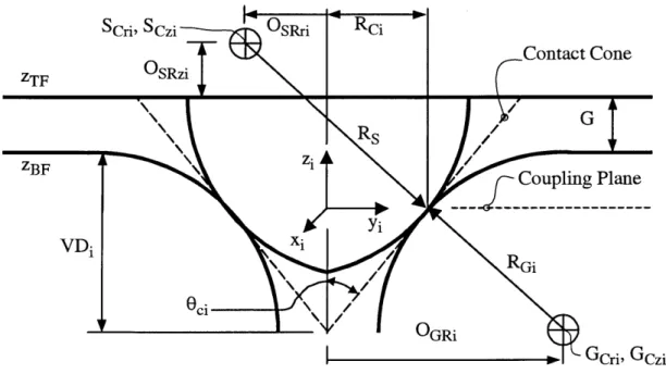
A cross section of a QKC joint is shown in Figure 2.3. Each joint has a coordinate system in which the axis of symmetry for the contactors and targets is co-linear with the z axis of the joint coordinate system. The x and y axes of every joint coordinate system is placed in the coupling plane of the triangle which is defined by the plane through the nominal location of the contact arcs. Though this constrains the applicability of the coming analy-sis to planar couplings, this still encompass the majority of coupling applications.
SCri, SCzi 'OSRri
OSRzT -Rci RS zi Yi . Xi 0 ci-Contact Cone
Figure 2.3 Placement of Joint Coordinate System and Variables For Joint i
Each joint has a contact cone. This is the surface defined by the tangents to the contactors and targets at cross sections through the axis of symmetry. In the 2D case shown in Fig.2.3, it appears as a "V", but since the elements contact over an arc in three dimensional
ZTF ZBF VE 0 I 35 X G COUPling Plane RGi GRi - GCri, Gczi
space, the actual shape is a cone. This cone is very important as half its included angle
(60) is used extensively in the calculation of QKC stiffness. We shall cover this in more detail in Chapter 3.
Several variables which describe characteristics of QKC joints are defined via Figure 2.3. The most important are:
* VD -Depth of the contact cone
e G -Gap, or distance between opposing faces of coupled components - RG -Groove radius at contact point
" Rs -Sphere radius at contact point
" OSR - Offset of groove radius from center line
* OGR - Offset of groove radius from center line
Note that some variables appearing with the subscript r, i.e. SCr and GCr, would seem to be redundant. The r subscript signifies that these values are invariant with respect to x and y and have been defined using a radial coordinate within the x-y plane specified from the joint coordinate system. This is in contrast to their "redundant" counterparts, OSR and OGR, which must retain their sign for use in some calculations. Note that variables which can either be positive or negative are shown using one sided arrows. The direction of the arrow with respect to left or right of the axis of symmetry provides the sign of the quantity, left is negative. For example, in Figure 2.3, OSR is shown as negative, while OGR is shown as positive. For a convex groove, OGR would be negative.
2.2.2
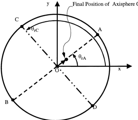
Analytic Components of Coupling
The coupling triangle is defined by lines which connect the joint coordinate systems as shown in Fig.2.4. The coupling centroid is defined as the intersection of the angle bisec-tors of the included angles of the coupling triangle. A coordinate system, the centroid coordinate system, is placed at this location. Note that these analytic components exist for each of the coupled components and are initially coincident. After geometric or force
dis-Analytic Components of QKCs 37
turbances, these coordinate systems will separate. The linear and angular movements between these coordinate systems are used to describe the error between the components.
Coupling Centroid C l
1
Y 3 -- 0
Angle Bisector 2
X2
Figure 2.4 Analytic Components of A Quasi-Kinematic Coupling
2.2.3 Contact Angle
Each contactor-target contact arc sub-tends an angle called the contact angle, OeC as shown in Fig.2.5. As the contact angle decreases, the arcs of contact become smaller, approaching point contact in the limit as Ocr goes to zero.
Groove Relief
Target Contact Surface
2.3 Function of Quasi-Kinematic Couplings
Due to friction and surface irregularities (Slocum, 1992a), when the coupling components are first mated as in Figure 2.6-A, the components will not occupy the most stable equilib-rium. Proper seating can be achieved by a preload that overcomes the contact friction and causes the spherical elements to brinell out surface irregularities at the contacts (Culpep-per et. al., 1999a).
JPRELOAD
...---- E L--A D-IP ...
A B C
Sinitiae-- Sinal
01,~
Figure 2.6 Mating Cycle of Quasi-Kinematic Couplings
If mating of opposed faces is desired, i.e. for sealing or stiffness, the gap between compo-nents and the compliance of the kinematic elements can be chosen such that the preload will close the initial gap, 8initial as shown in Fig.2.6-B. On removal of the load, all or part of the gap is restored through elastic recovery of the kinematic elements, thereby preserv-ing the kinematic nature of the joint for subsequent mates. If the initial deformation is elastic, the whole gap will be restored. If elastic and plastic, only a portion of the gap will be recovered.
With the gap closed, high stiffness can be achieved. This is due to the fact that the cou-pling stiffness becomes dependent on the interaction of the opposing surfaces, not the quasi-kinematic interfaces. As such, the stiffness in the direction perpendicular to the plane of the mated surfaces depends primarily on the stiffness of the clamping method. The stiffness in directions contained in the plane of the mated surfaces, i.e. the plane of mating, depends on the contact friction between the components and the load used to press them into contact (Culpepper et. al., 1998).
Chapter 3
MODELING AND ANALYSIS OF
QKCS
3.1 Modeling of Quasi-Kinematic Couplings
As explained in Section 2.3, these couplings operate on principles which are fundamen-tally different from those which govern the behavior of traditional kinematic couplings. As such they exhibit unique characteristics, some of which contradict classical kinematic coupling theory. For instance the posses the ability to align the grooves to provide maxi-mum stiffness in one direction. The following sections review the traditional kinematic coupling solution process, explains why a new process is needed, then presents a means to model and analyze the behavior of QKCs.
3.1.1 Kinematic Coupling Solution
It is beneficial to understand how one analyzes a traditional hard mount kinematic cou-pling before attempting to analyze a QKC. Given the geometry, material, and applied loads, one can model these couplings and find a closed form solution (Slocum, 1992a). Figure 3.1 shows the general solution procedure. It is not possible to determine relative movement between the components without considering the interaction at the contacts. Therefore, the determination of the contact forces and displacements is necessary.
Consider the Kinematic Coupling of Fig.3.2 in static equilibrium. Were a combination of forces and torques applied to the top component, reaction forces would the develop at the
Geometry Applied Interface Denections Relative Material =0 Loads n* Forces 5 -> Ar Error
[Fp & No] [Fl]
Figure 3.1 Solution Procedure For Kinematic Couplings
point contacts. A solution to the problem consists of the direction and magnitude of the individual contact force vectors. For each contact force vector, the direction of the vector is described by three independent quantities and the magnitude of the vector by one. This yields 24 (6 x 4) quantities which must be solved for.
- - -
--Figure 3.2 Traditional Hard Mount Kinematic Coupling
Basic free body diagram analysis tells us that the contact forces will be perpendicular to the groove surfaces if one can assume the coefficient of friction at the contact interfaces is small. As we know the geometry of the grooves, we can determine the direction of the contact forces. This is an important characteristic of kinematic couplings, which quasi-kinematic couplings do not posses.
Modeling of Quasi-Kinematic Couplings
With the directions of the forces known, only the magnitude of the six contact forces need be determined. The six force and moment equilibrium equations can be used to determine these forces, which are then used to calculate the hertzian deflections between the balls and grooves. Knowing these deflections, one can estimate the relative movement of the mated components (see Slocum, 1992a for further detail).
3.1.2 Solving the QKC Over Constraint Problem
Since QKCs rely on arc, not line or point contact, it is not possible to know a priori the direction of the reaction forces between the contactors and targets. This leaves 24 unknowns, six equilibrium equations, and one equation for the minimization of stored energy. There are more unknowns than equations, making solution in closed form impos-sible. However, one can reverse part of the process used by kinematic coupling to esti-mate the stiffness of the coupling. This is shown in the context of the kinematic coupling solution procedure of Fig.3.3 and represented by the formal QKC solution process shown in Fig.3.4
Geometry Applied Resultant Deflections Relative Matril 1* Loads Forces 's >,&rrr
[Fp & IV] [ni & Fi]
Figure 3.3 Solution Procedure For Quasi-Kinematic Couplings In Context of Traditional Approach
Given the geometry, material properties of the coupling components, and contact stiffness, one can impose a displacement between the coupled components and use the contact stiff-ness (as a function of displacement) to determine the resultant forces between the contac-tors and targets. The applied loads are then calculated and used to determine the stiffness in the direction of the imposed displacement. Though this method is less desirable than a
Material Contact Stiffness -~ t Geometry Displacements -J
QKC Model
- Force/Torque p StiffnessIFigure 3.4 Stiffness Solution Model For Quasi-Kinematic Couplings
closed form solution, it provides enough information to make practical use of these cou-plings.
3.2 Quasi-Kinematic Coupling Contact Mechanics
No solutions for non-conforming axisymmetric arc contacts were found in the literature or through consultations with leading researchers in the field. The only reference of some help covered an iterative stiffness estimation for contact between a ball and a cone (Hale, 1999). This method is limited to applications with concentric contact of spheres and cones. It is not suitable for our analysis as one must be able to calculate the stiffness of the contactor-target interface when the axes of the contactor and target are misplaced by a small amount. Furthermore this method can not take into account interrupted contact between a contactor and target which occurs at the edge of the contactor/target surfaces, i.e. where the reliefs begin. This has led to the following analysis for determining the resultant force due to arc contact between non-conforming axisymmetric solids.
3.2.1 Contact Analysis Using a Rotating Coordinate System
The purpose of this section is to introduce the concept of a rotating coordinate system and explain why it is useful to our analysis. This is done in the context of an axisphere mated in a cone. This method can be
Quasi-Kinematic Coupling Contact Mechanics 43
extended to arc contact between general solids of revolution by replacing the cone in the following discus-sion with the contact cone (see Figure 2.3 on page 35).
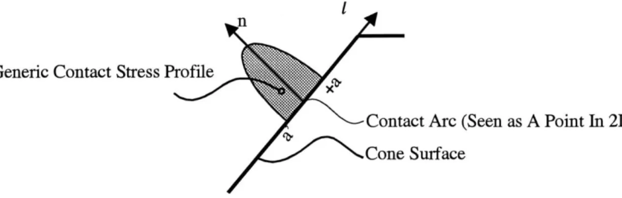
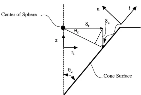
Consider the cross section of the cone shown in Fig.3.5. Were we to press a sphere or axi-sphere into a full cone, the arc of contact would be a circle. A conical coordinate system
Contact Stress Profile
Figure 3.5 Conical Coordinate System and Contact Stress Profile
consisting of unit vectors n, 1, and s, is placed coincident with the arc of contact and orien-tated such that the n vector is normal to the cone surface and point toward the cone's axis of symmetry. The 1 vector points along the cone surface and away from the cone's vertex. The s vector is perpendicular to the s and 1 vectors and points in the direction of increasing 6r (Or is introduced below). The origin of the coordinate system is placed in the approxi-mate center of the contact stress profile as shown in Fig.3.6. The shortest distance from
n
Generic Contact Stress Profile
x§x
Contact Arc (Seen as A Point In 2D) Cone Surface
the cones axis of symmetry to the center of the contact arc is called the contact radius, Rc. It will be used to calculate the resultant force between the contactor and target.
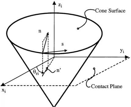
A symmetric contact profile is attained if friction is negligible and the material properties and the geometry of the contacting elements do not change much over the area of contact. Practically, the effects of friction will skew this profile to one side, however, it has been shown that in 2D line contact problems subjected to extreme engineering values, the effect of friction will be to skew the maximum of the contact stress profile by approximately six percent of the width of the contact zone (Johnson, 1985). In the case of large coefficients of friction, the profile may not be symmetric, but positioning it about the "frictionless line of symmetry" will introduce little error in the value of Rc. Typically the shift is on the order of 6 - 10 % of the profile width, which is much smaller than the contact radius, Rc. We plan to integrate the stress profile to obtain the force between the cone and groove. To capture the contribution of all points along the arc, the n-l-s coordinate system is allowed to rotate around the axis of symmetry of the cone during an integration. This will be explained later in Section 3.3.1, but for now it is enough to know that the coordinate sys-tem rotates. This rotation is defined by the angle 0r which is the angle between the vector
n' and the x axis of a Cartesian coordinate system whose z axis is co-linear with the axis of symmetry of the cone. This is illustrated in Fig.3.7. Note that the n' vector is the compo-nent of the n vector in the x-y plane.
If given the stress profile in Conical coordinates, i.e. as a function of Or, one can obtain the resultant force relative to the joint's frame of reference (Cartesian) by transforming the Conical coordinates to Cartesian coordinates, then integrating the modified function over
0r. The transformation, the Culpepper Transformation, required to do this is provided in
Equation 3.1. The use of this equation will be further explored in Section 3.2.2.
n -COS(Or)cos(Oc) -sin(Or)cos(Oc) sin(OC)
^I = ~-Sin(,) Cos(0) 0 (3.1)
Quasi-Kinematic Coupling Contact Mechanics
Cone Surface
yi
-- 0
Contact Plane
Figure 3.7 Rotating Conical Coordinate System At Joint i
3.2.2 Relationship Between Surface Stresses and Force Per Unit Length
The goal of this section is to discuss how the contact stress profile, force per unit length, and friction are related analytically. These relations will be used in section 3.3.1 to calculate the resultant force between the contactor and targets.
Contact Stress
The contact stress profile can be integrated to determine the force per unit length of con-tact. This can be done for any surface contact profile, elastic or plastic.
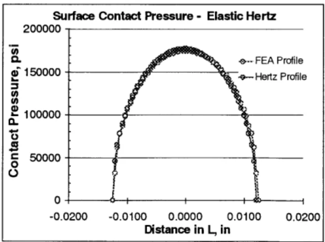
we will use an elastic Hertzian contact profile of the form:
As an example,
(3.2)
2fn(Or) I /
CVl, Or) = ' 1- ^
a,
Integrating Equation 3.2 gives the expected result:
( 2) 1/2 a 2f-(O) (,^ di -a a2 (3.3) 45 Zi n s Ori W Xi
Friction Induced Traction
Friction is a complicated phenomena. It is the analytic embodiment of energy dissipation through (Suh, 1993):
- Adhesion of contacting materials
* Plowing by wear particles and asperities
* Plastic working of the asperities, contacting surfaces, and trapped particles
In our analysis, we will consider friction caused by plowing of wear particles and plastic working of asperities, contacting surfaces, and trapped particles. Adhesion typically plays a minor role, especially where contaminants, i.e. oil, cutting fluid, and oxide layers pre-vent adhesion and low temperatures do not act to breakdown surface oxide layers.
Following the approach of Section 3.2.1, we assume friction has little affect on the contact stress profile. Note, if this were not the case, one could change the limits of the following integral to adjust. It is then possible to describe the friction forces in the s and 1 directions using Amonton's Law of Friction. In our case it is:
f(Or) =
f
-i Cy (1, Or)dl = jdn(Or)l (3.4)-a Ti n
Note the subscript i denotes the friction force per unit length in either the s or 1 direction.
3.2.3 Far Field Distance of Approach
The goal of this section is to develop the equations for transforming imposed displacements (supplied by the user) in cartesian coordinates to a form which can be used in the next section to calculate the resultant forcesfrom these displacements.
Far field distance of approach or distance of approach is a term frequently used in contact analysis. It is the change in distance between two far field points in contacting elements. Far field implies that the points are far from the contact region, meaning far from any points experiencing significant strain, say approximately 5% of the strain due to the con-tact. The intersection of our axisphere's radius with the z axis will serve as one point, the
Quasi-Kinematic Coupling Contact Mechanics
other must be chosen along the line from the sphere center to the contact area. This point is subject to the strain constraint discussed above. Note that the distance of approach is not the compression of the surfaces at the contact interface. Determining this can be a complicated task and it does not take into account the strain away from the contact zone. For our purposes, working with the distance of approach is much simpler and still pro-vides a general solution.
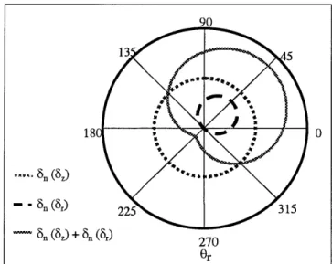
In learning how to make use of supplied displacements, we will first seek understanding through a qualitative description. Consider a sphere which is seated in a cone. Due to the axisymmetric nature of the problem, we can think of this as a series of 2D problems of cross sections of the axisphere-cone joint. When we press the axisphere into the cone, or in the -z direction, the distance of approach between the center of the sphere and far field points in a particular cross section will be equal for every cross section through the cone's axis of revolution. In other words, the distance of approach will be constant with Or This is shown in Fig.3.8 as 8n(Sz)-90 13 45 18 0-6n1 (8~) -6 .0(8) 225 315 8n (8z) + 6. (6) 270 Fr
Figure 3.8 Normal Distance of Approach of Two Far Field Points In Mated Contactor and Target