HAL Id: inria-00562326
https://hal.inria.fr/inria-00562326
Submitted on 3 Feb 2011
HAL is a multi-disciplinary open access
archive for the deposit and dissemination of
sci-entific research documents, whether they are
pub-lished or not. The documents may come from
teaching and research institutions in France or
abroad, or from public or private research centers.
L’archive ouverte pluridisciplinaire HAL, est
destinée au dépôt et à la diffusion de documents
scientifiques de niveau recherche, publiés ou non,
émanant des établissements d’enseignement et de
recherche français ou étrangers, des laboratoires
publics ou privés.
Image Classification by Finite Mixtures and Copulas
Vladimir Krylov, Gabriele Moser, Sebastiano B. Serpico, Josiane Zerubia
To cite this version:
Vladimir Krylov, Gabriele Moser, Sebastiano B. Serpico, Josiane Zerubia. Supervised High Resolution
Dual Polarization SAR Image Classification by Finite Mixtures and Copulas. IEEE Journal of Selected
Topics in Signal Processing, IEEE, 2011, �10.1109/JSTSP.2010.2103925�. �inria-00562326�
Supervised High Resolution Dual Polarization SAR
Image Classification by Finite Mixtures and Copulas
Vladimir A. Krylov, Gabriele Moser, Member, IEEE, Sebastiano B. Serpico, Fellow, IEEE,
and Josiane Zerubia, Fellow, IEEE
Abstract—In this paper a novel supervised classification ap-proach is proposed for high resolution dual polarization (dual-pol) amplitude satellite synthetic aperture radar (SAR) images. A novel probability density function (pdf) model of the dual-pol SAR data is developed that combines finite mixture modeling for marginal probability density functions estimation and copulas for multivariate distribution modeling. The finite mixture modeling is performed via a recently proposed SAR-specific dictionary-based stochastic expectation maximization approach to SAR amplitude pdf estimation. For modeling the joint distribution of dual-pol data the statistical concept of copulas is employed, and a novel copula-selection dictionary-based method is proposed. In order to take into account the contextual information, the developed joint pdf model is combined with a Markov random field approach for Bayesian image classification. The accuracy of the developed dual-pol supervised classification approach is validated and compared with benchmark approaches on two high resolution dual-pol TerraSAR-X scenes, acquired during an epidemiological study. A corresponding single-channel version of the classification algorithm is also developed and validated on a single polarization COSMO-SkyMed scene.
Index Terms—Polarimetric synthetic aperture radar, super-vised classification, probability density function (pdf), dictionary-based pdf estimation, Markov random field, copula.
I. INTRODUCTION
I
N MODERN remote sensing, the use of synthetic aperture radar (SAR) represents an important source of information for Earth observation. Recent improvements have enabled modern satellite SAR missions, such as COSMO-SkyMed and TerraSAR-X, to acquire high resolution (HR) data (up to metric resolution) with a very short revisit time (e.g. 12 hours for COSMO-SkyMed). In addition, SAR is robust with respect to lack of illumination and atmospheric conditions. Together, these factors explain the rapidly growing interest in SAR imagery for various applications, such as flood/fire monitoring, urban mapping and epidemiological surveillance. Classification is one of the most important image processingThis research was a collaborative effort between the Institut National de Recherche en Informatique et en Automatique (INRIA) Sophia Antipolis -M´editerran´ee Center, France, and the Dept. of Biophysical and Electronic Engineering (DIBE) of the University of Genoa, Italy. It was carried out with the partial financial support of the INRIA and the French Space Agency (CNES).
V.A. Krylov is with the Faculty of Computational Mathematics and Cy-bernetics, Lomonosov Moscow State University, 119991, Moscow, Russia, and also with the EPI Ariana, INRIA/I3S, F-06902, Sophia Antipolis Cedex, France (e-mail: [email protected]).
G. Moser, S.B. Serpico are with DIBE, University of Genoa, I-16145, Genoa, Italy (e-mail: [email protected], [email protected]).
J. Zerubia is with the EPI Ariana, INRIA/I3S, F-06902, Sophia Antipolis Cedex, France (e-mail: [email protected]).
tasks applied to remote sensing imagery. Classification maps can either be directly used in applications or they can serve as an input to further SAR processing problems, e.g., for change detection.
Contemporary satellite SAR missions are capable of provid-ing polarimetric imagery, which provide a more complete de-scription of landcover scattering behavior than single-channel SAR data [1], [2]. The potential for improved classification accuracy with data in several polarizations, compared to single-channel data, explains the special interest to polari-metric SAR image classification. Furthermore, several current satellite SAR systems, e.g., TerraSAR-X, COSMO-SkyMed, support, at least, dual-pol acquisition mode. In this paper we investigate the dual polarization (dual-pol) SAR imagery scenario, as well as single polarization (single-pol) SAR, as a special case.
A wide variety of methods have been developed earlier for the classification of polarimetric SAR data [2]. We list some recent methods based on the employed methodological approach: maximum likelihood [3]–[7], neural networks [8], [9], support vector machines [10], fuzzy methods [11], [12], stochastic complexity [13], spectral graph partitioning [14], wavelet texture models [15] and other approaches [16], [17]. In this paper we develop a classification method based on the maximum likelihood approach. As such, this method specifies a probability density function (pdf) describing the statistics of polarimetric SAR data. Previously, several models have been proposed for this purpose: the classical Wishart distri-bution [3], [18], the K-distridistri-bution [4], [19] for textured areas, the K-Wishart distribution [6] designed to improve the distin-guishability of non-Gaussian regions, the G-distribution [5], [20] for extremely heterogeneous areas, the Ali-Mikhail-Haq copula-based model [21] combined with the Sinclair matrix representation, and the KummerU distribution [7] for Fisher distributed texture. These models were developed for the multilook complex-valued SAR image statistics. In this paper, we study SAR classification using only the amplitude data and not the complex-valued data. This is an important data typology because several image products provided by novel high resolution satellite SAR systems are geocoded ellipsoid-corrected amplitude (intensity) images, and because several earlier coarser resolution sensors (e.g., ERS) primarily used this modality.
The classification technique developed in this paper com-bines the Markov random field (MRF) approach to Bayesian image classification with the dictionary-based stochastic ex-pectation maximization (DSEM) amplitude pdf estimator.
MRFs represent a general family of probabilistic image models that provide a convenient and consistent way to characterize context dependent data [22]. The latter has been developed for the purpose of modeling the amplitude distributions of SAR images [23], [24]. Contrary to various pdf models [1], [25]–[30], DSEM uses a mixture of several distinct SAR-specific pdfs to accurately model the amplitude statistics. The benefit of using the finite mixture DSEM approach is twofold: First, DSEM is an efficient and automatic tool for SAR amplitude pdf estimation, capable of providing estimates of higher accuracy than single parametric pdf models, and, second, the underlying mixture assumption in DSEM enables accurate characterization of the inhomogeneous classes of interest, i.e., classes which contain several different landcover subclasses. This is particularly important for HR imagery. The resulting DSEM-MRF technique is a simple and efficient tool for single-channel SAR classification. In order to support dual-pol SAR data, copula theory is used for modeling the joint class-conditional distributions of the dual-pol channels, re-sulting in a Copula-DSEM-MRF approach (CoDSEM-MRF). The employed joint distribution modeling tool, copulas [31], is a rapidly developing statistical tool that was designed for constructing joint distributions from marginals with a wide variety of allowable dependence structures. For every class the choice of an optimal copula from a dictionary of copulas is performed by a dedicated criterion. The concept of copulas is relatively new in image processing, and has just emerged in remote sensing methods [21], [32], [33]. The approach suggested in [21] can also be used for dual-pol SAR and it is compared with the developed in this paper technique in Section IV. The proposed CoDSEM-MRF HR dual-pol SAR classification technique is based on three flexible statistical modeling concepts, i.e. copulas, finite mixtures and MRFs, and constitutes an efficient and robust approach with respect to possibly sophisticated classes of interest.
The contributions of this paper are twofold: First, we de-velop a novel single-channel HR SAR classification approach that is based on SAR-specific DSEM probability density function estimation technique and a contextual MRF model, and, second, we use a novel parametric statistical modeling approach, which is based on a dictionary of copulas, to de-velop a dual-pol HR SAR classification method. This method outperforms benchmark approaches, such as the parametric 2D Nakagami-Gamma [18] model combined with MRF, and the nonparametric “K-nearest neighbors” [34] method combined with MRF.
This paper is organized as follows. In Section II, we present an overview of the developed DSEM-MRF and CoDSEM-MRF approaches to HR SAR classification. In Section III, the description of methodological components of the designed approach, i.e., the DSEM approach to amplitude pdf estimation and bivariate copulas, are presented. Section IV reports the experiments of the developed SAR classification approach on HR dual-pol TerraSAR-X and single-pol COSMO-SkyMed images. Conclusions are drawn in Section V.
II. METHOD OVERVIEW
In this section, we present an overview of the developed CoDSEM-MRF approach to dual-pol SAR classification. We treat single-channel SAR classification (DSEM-MRF) as a special case of SAR classification. The first two steps of the algorithm (the DSEM and Copula steps) are presented in more detail in the next section.
A. Dual-pol case
In this subsection, we present the key steps of the proposed CoDSEM-MRF classification algorithm for the case of dual-pol SAR (2 dual-polarization channels). We study supervised clas-sification with M classes of interest. Thus we assume training pixels for these classes to be available.
DSEM step. In the first step, the marginal pdfs of polar-ization channels are estimated separately by applying DSEM to the training pixels available for the considered classes of interest. For each m-th class and d-th channel (m = 1, . . . , M ,
d = 1, 2), the mixture DSEM pdf estimators pdm(yd|ωm) and
the corresponding cumulative distribution functions (CDFs)
Fdm(yd|ωm) are as follows: pdm(yd|ωm) = KXdm i=1 Pdmipdmi(yd), Fdm(yd|ωm) = KXdm i=1 PdmiFdmi(yd), (1)
where ωmis the event of the observation belonging to the m-th
class, y1 and y2 are the amplitudes from the two polarization
channels and Kdm is the number of components in the
mixture. Fdmi and pdmi represent the i-th mixture component
in the CDF and pdf domains, respectively, and Pdmi is the
related mixture proportion; pdmi is automatically drawn by
DSEM from a dictionary of several SAR-specific parametric pdfs, i = 1, . . . , Kdm. There are two reasons why DSEM was
used instead of a single parametric pdf model. First, DSEM is an efficient and automatic tool for SAR amplitude pdf estimation, and it is capable of providing estimates of higher accuracy compared to single parametric pdf models [23], [24]. Specifically, DSEM was experimentally found to accurately estimate the statistics of a HR satellite SAR image [24]. Second, the underlying mixture assumption in DSEM enables accurate characterization of the inhomogeneous classes of interest, i.e., the classes that contain several different landcover subclasses. This is a very important property when dealing with HR imagery, since the corresponding image statistics are usually strongly mixed due to the high level of spatial detail appreciable at high resolution. However, even in the case of homogenous classes, DSEM can be viewed as a tool for choosing the best single pdf model from the set of pdfs in the DSEM dictionary.
Copula step. The goal of this step is to merge the marginal pdfs, which correspond to polarization channels estimated on DSEM-step, into a joint bivariate pdf describing the joint amplitude distribution of the dual-pol SAR image. To this end, the joint pdfs pm(y1, y2|ωm) for classes m = 1, . . . , M are
modeled via copulas from the marginal distributions in Eq. (1). The choice of copulas as a tool for joint distribution estimation is attractive because of the simplicity in its analytical formulations, and because a wide variety of dependence structures can be modeled. Thus, joint pdfs are constructed as:
pm(y1, y2|ωm) = p1m(y1|ωm)p2m(y2|ωm) × ∂ 2C∗ m ∂y1∂y2(F1m(y1|ωm), F2m(y2|ωm)), (2) where C∗
m is a specific copula for the m-th class and is
au-tomatically picked by the algorithm from a dictionary of con-sidered copulas (m = 1, . . . , M ; details are found in Sec. III). MRF step. In order to take into consideration the contex-tual information disregarded by the pixel-wise Copula-DSEM technique, and to gain robustness against the inherent noise-like phenomenon of SAR known as speckle, we adopted a contextual approach based on an MRF model. Following the classical definitions of MRFs (see, e.g., [35], [36]) on the two dimensional lattice S of N observations y = {y1, . . . , yN}
and class labels x = {x1, . . . , xN}, xi ∈ {1, . . . , M }, we
introduced an isotropic second-order neighborhood system C with cliques of size 2. The Hammersley-Clifford theorem [36] allows for the presentation of the joint probability distribution of an MRF as a Gibbs distribution:
P (x) = Z−1exp(−H(x|β)),
where Z = Pzexp(−H(z|β)) is a normalizing constant,
β is a positive parameter and H(x|β) is the MRF energy
function of the class labels. More specifically H(x|β) takes the following form:
H(x|β) = X {s,s0}∈C £ −β δxs=xs0 ¤ ,
where δ is the Kronecker delta:
δxs=xs0 =
(
1, if xs= xs0
0, otherwise.
Image classification poses a problem of recovering the unobserved data, i.e., class labels. In the case of hidden MRFs, the unobserved data x are modeled by an MRF and the observed data y, i.e., SAR amplitudes, are assumed to be conditionally independent given x [35]:
p(yi|yS\{i}, xi) = p(yi|xi), ∀i ∈ S,
where yi is the pair (y1, y2) at pixel i, y = {y1, . . . , yN},
and S \ {i} represents all the pixels of S except i. Thus, given the conditional pdfs in Eq. (2), we model the full data (y, x) as a hidden MRF with the energy function:
U (x|y, β) =X i∈S Ui(xi|yi, xS\{i}, β), (3) where for m = 1, . . . , M : Ui(xi= ωm|yi, xS\{i}, β) = − log pm(yi|ωm) − β X s:{i,s}∈C δxi=xs. (4)
The energy function in Eq. (3) has a single parameter β that must be estimated. Conveniently, all of the parameter estimation involved in Eq. (1) is incorporated into DSEM. Thus, the resulting energy function (1)-(3) also has only one parameter. In order to estimate β, we used a simulated annealing procedure [37] with a pseudo-likelihood function
P L [36] of the following form:
log P L(x|β) = log " Y s∈S P (xs|xS\{s}, β) # , where: P (xs|xS\{s}, β) = exp(−U (xs|xS\{s}, β)) P zs∈XS exp(−U (zs|xS\{s}, β)) , and Xs= {ω1, . . . , ωM}.
The implemented simulated annealing procedure generated a sequence {βt} of estimates, and employed the normal
pro-posal distribution N (βt, 1) [38] together with an exponentially
decreasing cooling schedule Tt = 0.95 · Tt−1. Considering
the convergence in distribution of the related Metropolis algo-rithm, the final estimate β∗was set by averaging the estimates
on the last n iterations. The estimation of β was performed on an ML pre-classification of the image, which associated every pixel with the highest probability-density label according to the Copula-DSEM models.
Energy minimization step. This step involves the mini-mization of the energy in Eq. (3). For this optimini-mization prob-lem the iterative deterministic modified Metropolis dynamics (MMD) [40] algorithm was adopted. This is a compromise between the deterministic “iterated conditional modes” algo-rithm (ICM) [36], which is a fast local minimization technique, that is strongly dependent on the initial configuration, and simulated annealing (SA) [37], which is a very computa-tionally intensive global minimization approach. MMD is computationally feasible and provides reasonable results in real classification problems [40]. MMD is set with a cooling schedule (like SA) and proceeds as follows:
1. sample a random initial label configuration x0, define an
initial temperature T0and parameters α ∈ (0, 1), n 1∈ N,
τ ∈ (0, 1), γ ∈ R+, initialize k = 0 and T 0= T0; 2. set i = 0;
3. using uniform distribution pick up a label configuration
η which differs exactly in one element from xk;
4. compute ∆ = U (η) − U (xk) and accept η according to
the rule: xk+1= η, if ∆ 6 0 η, if ∆ > 0 and ln(α) 6 −∆ Tk xk, otherwise ; 5. calculate ∆Ui= |U (xk+1) − U (xk)|;
6. if i 6 n1, set i = i + 1 and goto Step 3; 7. calculate ∆U =Pn1
i=1∆Ui;
8. if ∆U/U (xk+1) > γ decrease the temperature T k+1 =
τ Tk, increase k = k +1, and goto Step 2; stop otherwise.
During the early stages of this iterative procedure, the behavior of MMD is close to that of SA, and thus it provides much better exploratory properties as compared to ICM.
TABLE I
PDFS ANDMOLCEQUATIONS FOR THE PARAMETRIC FAMILIES INCLUDED IN THE CONSIDERED DICTIONARYDM: LOG-NORMAL, WEIBULL,
NAKAGAMI ANDGENERALIZEDGAMMA(GΓD)DISTRIBUTIONS. HEREΓ(·)IS THE GAMMA FUNCTION, Ψ(·)THE DIGAMMA FUNCTION ANDΨ(ν, ·)
THEνTHORDER POLYGAMMA FUNCTION[39]
Family Probability density function MoLC equations Log-normal f1(r|m, σ) = σr√12πexp h −(ln r−m)2σ2 2 i , r > 0 κ1= m κ2= σ2 Weibull f2(r|µ, η) =µηηrη−1exp h −³r µ ´ηi , r > 0 κ1= ln µ + Ψ(1)η−1 κ2= Ψ(1, 1)η−2 Nakagami f3(r|λ, L) =Γ(L)2 (λL)Lr2L−1exp ¡ −λLr2¢, r > 0 2κ 1= Ψ(L) − ln λL 4κ2= Ψ(1, L) GΓD f4(r|κ, σ, ν) =σΓ(κ)ν ¡r σ ¢κν−1 exp©−¡r σ ¢νª , r > 0 κ1= Ψ(κ)/ν + ln σ κj= Ψ(j − 1, κ)/νj, j = 2, 3 B. Single-pol case
Here we consider single-pol classification as a particular case of the developed algorithm. In this case the target joint pdf is univariate. Thus there is no need for the Copula-step, because the DSEM-step estimates provide the goal pdfs and can be directly plugged into Eq. (3) in the MRF-step. In the single-pol case the algorithm (DSEM-MRF) represents the straightforward application of the DSEM technique to MRF-based SAR image classification.
III. METHODOLOGICAL COMPONENTS
A. Dictionary-based Stochastic Expectation Maximization
In this subsection, we present the outline of DSEM. This ap-proach was initially developed in [23] for medium-resolution SAR and then enhanced and validated on high resolution SAR in [24].
To take into account the heterogeneity, when several distinct land-cover typologies are present in the same SAR image, a finite mixture model [41] for the distribution of grey levels is assumed. Specifically, DSEM is applied to estimate marginal class-conditional statistics. Separately focusing on each class
ωm and each channel yd, m = 1, . . . , M , d = 1, 2, dropping
the subscripts m and d for ease of notation, and denoting
yd simply as r, we assume that the d-th component of
the training samples of ωm are independent and identically
distributed random variables, drawn from a mixture pdf with
K components: p(r) = K X i=1 Pipi(r), r > 0, (5)
where pi(·) is the i-th mixture component and {Pi} is a set
of mixing proportions, i.e., PKi=1Pi= 1 and 0 6 Pi6 1 for
i = 1, . . . , K. Each component pi(·) is modeled by resorting
to a finite dictionary DM = {f1, . . . , f4} (see Table I) of four
SAR specific distinct parametric pdfs fj(r|θj), parameterized
by θj ∈ Aj, j = 1, . . . , 4 [24]. Assuming that channel r is
quantized on the levels {0, 1, . . . , Z − 1}, we also denote by
h(z), z = 0, . . . , Z − 1, the histogram of r, when restricted to
the training samples of the considered class.
The calculation of CDFs is needed to merge the marginal DSEM pdf estimates of polarization channels into joint pdfs via copulas (see Eq. (2)). Therefore, the pdfs in the dictionary have been chosen so that, for each of them, there is either an analytical closed-form expression (f1, f2), or a simple
numerical approximation procedure (f3, f4) for the related
CDF. For the rest of the models considered in [24], where the dictionary includes also Fisher [27], K-root [25], generalized Gaussian-Rayleigh [29] and symmetric-α-stable generalized Rayleigh [28] pdf models, there are no closed-form CDFs and numerical approximation is computationally intensive. Furthermore, the experiments in [24] demonstrate that very accurate pdf estimates can be obtained with this dictionary of four models. Therefore, the dictionary DM considered in this
paper has been restricted to the four models in Table I. As discussed in [23], considering the variety of estimation approaches for finite mixtures, the appropriate choice for this particular estimation problem is the iterative stochastic expec-tation maximization (SEM) scheme [42]. Instead of adopting ML estimates as the classical SEM scheme suggests [42], DSEM employs the Method of Log-Cumulants (MoLC) [27], [43] for component parameter estimation, which has been demonstrated to be a feasible and effective estimation tool for all the pdfs in DM [23], [24], [27], [30]. The MoLC equations
relate the unknown pdf parameters with κ1, κ2 and κ3:
(
κ1= E{ln r}
κj = E{(ln r − κ1)j}
, j = 2, 3,
which are the 1st, 2nd, 3rd order logarithmic cumulants,
re-spectively. The MoLC equations have a single solution for any observed values of log-cumulants for all pdfs in DM
(see Table I). MoLC equations for f1 and f2 allow analytical
solutions. For f3and f4, the strict monotonicity of the involved
functions allows solutions to be reached by numerical proce-dures. As in [24], we implemented a K-estimation procedure that consists of initializing SEM with K0= K
max, and then
allowing components to be eliminated from the mixture during the DSEM iterative process, once their priors become too small, thus decreasing K.
TABLE II
CONSIDERED DICTIONARYDCOF COPULAS: CLAYTON, ALI-MIKHAIL-HAQ, GUMBEL, FRANK, A12, A14, FARLIE-GUMBEL-MORGENSTERN(FGM),
MARCHAL-OLKIN, GAUSSIAN ANDSTUDENT-T,EACH DEFINED BY THE FUNCTIONCc(u, v|θ) (c = 1, . . . , 8),ALONG WITH THEθ(τ )DEPENDENCIES ANDτ -INTERVALS. HEREφ−1(t)ANDt−1
ν (t)DENOTE THE QUANTILE FUNCTIONS OF A STANDARD UNIVARIATE NORMAL AND A STANDARD UNIVARIATEtνDISTRIBUTIONS RESPECTIVELY.
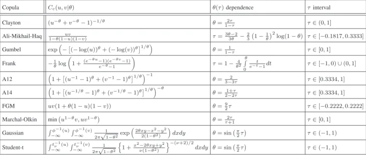
Copula Cc(u, v|θ) θ(τ ) dependence τ interval
Clayton (u−θ+ v−θ− 1)−1/θ θ = 2τ 1−τ τ ∈ (0, 1] Ali-Mikhail-Haq uv 1−θ(1−u)(1−v) τ = 3θ−2 3θ − 2 3 ¡ 1 −1 θ ¢2 log(1 − θ) τ ∈ [−0.1817, 0.3333] Gumbel exp³−£(− log(u))θ+ (− log(v))θ¤1/θ´
θ = 1 1−τ τ ∈ [0, 1] Frank −1 θlog µ 1 +(e−θu−1)(ee−θ−1−θv−1) ¶ τ = 1 − 4 θ2 θ R 0 t e−t−1dt τ ∈ [−1, 0) ∪ (0, 1] A12 ³ 1 +£(u−1− 1)θ+ (v−1− 1)θ¤1/θ´−1 θ = 2 3−3τ τ ∈ [0.3334, 1] A14 ³1 +£(u−1/θ− 1)θ+ (v−1/θ− 1)θ¤1/θ´−θ θ = 1+τ 2−2τ τ ∈ [0.3334, 1] FGM uv(1 + θ(1 − u)(1 − v)) θ =92τ τ ∈ [−0.2222, 0.2222] Marchal-Olkin min¡u1−θv, uv1−θ¢ θ = 2τ τ +1 τ ∈ [0, 1] Gaussian R−∞φ−1(u)R−∞φ−1(v) 1 2π√1−θ2exp ³ 2θxy−x2−y2 2(1−θ2) ´ dxdy θ = sin¡π2τ¢ τ ∈ (−1, 1) Student-t Rt−1ν (u) −∞ Rt−1ν (v) −∞ 2π√11−θ2 n 1 +x2−2θxy+yν(1−θ2) 2 o−(ν+2)/2 dxdy θ = sin¡π 2τ ¢ τ ∈ (−1, 1)
• E-step: compute, for each greylevel z and i-th compo-nent, the posterior probability estimates corresponding to the current pdf estimates, i.e. z = 0, . . . , Z − 1:
τt i(z) = Pt ipti(z) PKt j=1Pjtptj(z) , i = 1, . . . , Kt;
• S-step: sample a component label st(z) ∈ {1, . . . , Kt} of each greylevel z according to the current estimated posterior probability distribution {τt
i(z) : i = 1, . . . , Kt},
z = 0, . . . , Z − 1;
• MoLC-step: for the i-th mixture component, compute the following histogram-based estimates of the mixture proportions and the first three log-cumulants:
Pit+1= P z∈Qith(z) PZ−1 z=0 h(z) , κt1i= P z∈Qith(z) ln z P z∈Qith(z) , κtbi = P z∈Qith(z)(ln z − κ t 1i)b P z∈Qith(z) , i = 1, . . . , Kt,
where b = 2, 3 and Qit = {z : st(z) = i} is the set of
grey levels assigned to the i-th component by the S-step; then, solve the corresponding MoLC equations (see Table I) for each parametric family fj(·|θj) (θj ∈ Aj) in the
dictionary, thus computing the resulting MoLC estimate
θt
ij, j = 1, . . . , 4;
• K-step: for each i = 1, . . . , Kt, if Pit+1is below a given threshold, eliminate the i-th component and update Kt+1;
• Model Selection-step: for the i-th mixture component, compute the log-likelihood of each estimated pdf fj(·|θtij)
according to the data assigned to the i-th component:
Ltij =
X
z∈Qit
h(z) ln fj(z|θijt), i = 1, . . . , Kt+1,
and define pt+1
i (·) as the estimated pdf fj(·|θtij) yielding
the highest value of Lt
ij, j = 1, . . . , 4.
B. Copulas
In this section, we present the employed dictionary of copulas and the novel copula selection procedure. An overview of bivariate copula concepts is presented in Appendix A.
We used copulas to model the joint distributions of a dual-pol SAR image, given estimates of the related marginal distri-butions [31]. As mentioned earlier, many parametric models have been proposed for marginal statistics of SAR amplitudes or intensities, but only a few models are available for the joint distribution of several SAR amplitudes, e.g. the Nakagami-Gamma model developed in [18]. In order to overcome this limitation, we combine the marginal pdfs provided by DSEM by means of copulas.
A bivariate copula is a 2-variate distribution defined on [0, 1]2 such that marginal distributions are uniform on [0, 1].
In this paper, we consider several parametric families of one-parameter copulas. By taking advantage of the connection of copulas with the Kendall’s tau ranking coefficient τ (see Ap-pendix A), we can obtain a closed-form relationship between τ and the copula parameter θ for each parametric copula. Given a sample-rank-statistics estimate of τ (Appendix A), an estimate of θ can be obtained by inverting the corresponding equation. In order to fully exploit the modeling potential of copulas, we consider a dictionary DC = {C1, . . . , C10} of 10
uni-parametric copulas Cc(u, v|θ) (0 ≤ u, v ≤ 1; c = 1, . . . , 10):
6 Archimedean (Clayton, Ali-Mikhail-Haq, Gumbel, Frank, A12, A14) [31], a copula with a quadratic section (Farlie-Gumbel-Morgenstern) [31], 2 elliptical (Gaussian and
Student-t1) [44] and a non-Archimedean copula with simultaneous
presence of an absolutely continuous and a singular component (Marchal-Olkin) [31]. Here the names for A12 and A14 originate from their positions in the list of Archimedean copulas in [31]. This choice of copulas is capable of modeling a wide variety of dependence structures, and covers most copula applications [45]. The considered dictionary of copulas is summarized in Table II (further information can be found in [31], [44], [45]).
The choice for every class m = 1, . . . , M of a specific copula C∗
m from the dictionary (see Eq. (2)) consists of the
following two steps. First, given an estimator ˆτ of τ (computed
with the training samples of the m-th class), one should decide whether a specific copula is appropriate for modeling the dependence with a corresponding value of Kendall’s tau rank correlation. Indeed, some copulas are specific to marginals with a low level of dependence, others deal with strongly dependent marginals, and still others are capable of modeling all levels of dependency. In other words, for each class, the list of copulas is limited to those which are capable of accurately modeling the specific empirically estimated value ˆ
τ (see Table II). Thus, we first discard the copulas for which
the current sample estimate ˆτ is outside the related τ -relevance
interval; for the remaining copulas, we derive an estimate ˆθ
of the related parameter by the above-mentioned Kendall’s tau method.
Second, for each class, we choose the copula with the high-est p-value in a Pearson chi-square thigh-est-of-fitness (PCS) [46]. In general, PCS tests the null hypothesis that the frequency distribution of certain events observed in a sample is consis-tent with a particular theoretical distribution. The chi-square statistic is constructed as follows:
X2= n X i=1 (Oi− Ei)2 Ei , (6)
where Oi and Ei are the observed and the hypothetical
frequencies, respectively, and n the number of outcomes. PCS is one of the statistical tests whose results are a chi-square distribution [46], i.e. X2 ∼ χ2
n−r−1, where r is the number
of reductions of degrees of freedom (typically, the number of parameters for parametric CDFs). The reference to χ2
distribution allows to calculate p-values for several different null hypothesis.
In our case, the null hypothesis in PCS is that the sample fre-quencies of the pairs of the form (F1m(y1|ωm), F2m(y2|ωm)),
as (y1, y2) varies in the set of training samples of the
m-th class, are consistent with the theoretical frequencies
(probabilities) predicted by the parametric copula Cc (m =
1, . . . , M ; c = 1, . . . , 10). This is correct because if x is distributed with CDF F (·), and x1, · · · , xN are independent
1Unlike all other considered copulas, the Student-t copula depends on two
parameters: the linear correlation coefficient θ and the number of degrees of freedom ν. To avoid a cumbersome ˆν ML estimation [44] we employ the following approach: we consider separately ν = 3k, with k from 1 to 9 due to the fact that as ν grows large (ν > 30) Student-t copula becomes indistinguishable from a Gaussian copula [44]. In other words, instead of a single biparametric Student-t copulas we consider here nine uniparametric Student-t copulas with fixed values of ν.
observations of x, then F (xi), i = 1, · · · , N , are independent
[0, 1]-uniformly distributed random variables [46]. IV. EXPERIMENTS
A. Datasets for experiments
The two versions of the algorithm, CoDSEM-MRF and DSEM-MRF, were tested on the following HR SAR datasets: • Dual-pol HH/VV TerraSAR-X, Stripmap (6.5 m ground resolution), geocorrected, 2.66-look image acquired over Sanchagang, China, in the framework of an epidemiology monitoring application ( c°Infoterra GmbH). We present
experiments on the 1000 × 1200 subimage TSX1 (see Fig. 1) and on the 750×750 subimage TSX2 (see Fig. 2). • Single-pol HH, 1-look COSMO-SkyMed (CSK°),R
Stripmap (2.5 m ground resolution), acquired over Piemonte, Italy ( c°ASI). We present experiments on the
700 × 1000 subimage CSK1 (see Fig. 3).
B. Experimental settings
The experiments involved the classification of humid re-gions into M = 3 classes: “water”, “wet”, and “dry soil”.
The following experimental settings were used. In the DSEM-step, given the relative homogeneity of the target
M classes on the experiment datasets, an average value of
the initial number of components K0 = 3 was selected,
thus assuming mixtures with just a few components for the classes. The threshold for component elimination on the K-step was 0.005 (as discussed in [24], the choice of this value only marginally affects the results). In the Copula-step, the following settings in the PCS test were used. The [0, 1]×[0, 1] square was divided into 25 equal squares Si by 4 horizontal
and 4 vertical lines parallel to the axes (i.e., n = 25). For every class m = 1, . . . , M and every cluster Si, i = 1, . . . , n:
Oim=
X
ISi[F1m(y1|ωm), F2m(y2|ωm)] ,
where I is the indicator function and the summation is taken over all the training pixels available for class m. For each copula c = 1, . . . , 10 in DC, the value of Eim was calculated
by integrating the related pdf over the square Si, thus retrieving
the probability that a pair of [0, 1]-uniform random variables, whose joint distribution is defined by the c-th copula, belong to Si (i = 1, . . . , n). In the Energy minimization step, the
revisit scheme on Step 3 of MMD was implemented raster-wise and the following parameter values were used : T0= 5.0,
α = 0.3, τ = 0.97, γ = 10−4 and n
1 was set equal to
the size of the image in pixels. Compared to ICM, MMD generated significantly better results (above 5% of accuracy gain), starting at ML initialization (maximizing Eq. (2) at each pixel). SA obtained slightly better results (roughly a 1% accuracy gain) compared to MMD. However, SA generated a drastic increase in computational complexity (around 200 iterations for MMD and over 1500 for SA).
For every dataset, the proposed algorithm was trained on a small 250×250 sub-image endowed with a manually annotated non-exhaustive ground truth (GT), that did not overlap with the test areas.
(a) TSX1 image, VV pol (b) manual GT (c) referenced 2DNG-MRF (d) referenced K-NN-MRF
(e) CoDSEM-MRF map (f) referenced CoDSEM-MRF (g) referenced DSEM-MRF on VV
(h) VV box (i) GT box (j) CoDSEM-MRF box (k) DSEM-MRF on VV box (l) K-NN-MRF box Fig. 1. (a) TSX1 image (1000 × 1200) in VV polarization and (h) its subimage (240 × 270). (b) and (i) manually created ground truth (GT), (e) CoDSEM-MRF classification map (water ¥, wet soil¥, dry soil¥). Classification maps referenced to the GT: (c) 2DNG-MRF, (d) and (l) K-NN-MRF, (f) and (j) CoDSEM-MRF, (g) and (k) DSEM-MRF on the VV pol image (correctly classified water ¥, wet soil¥, dry soil¥, misclassification of all types ¤).
C. Experimental results
Table III reports the accuracy obtained on the test samples for each class (“class accuracy”), the resulting average accu-racy (i.e., the arithmetic mean of the class accuracies) and overall accuracy (i.e., the percentage of correctly classified test samples, irrespective of their classes). The first test image TSX1 (see Fig. 1) covers an area of a river delta in San-chagang, China. For this experiment, an exhaustive ground truth was manually created, and the classification results were referenced to it in order to calculate the accuracies and demonstrate the results visually. The automatically selected copulas were: Gumbel for the “water”, and Frank for the
“wet soil” and “dry soil” classes. The β estimation provided
β∗ = 1.408 and the overall classification accuracy achieved
by CoDSEM-MRF was 84.5%. The resulting CoDSEM-MRF classification map is shown in Fig. 1(e) and referenced to the GT in Fig. 1(f).
In order to appreciate the classification gain from dual-pol data (HH/VV), compared to single-channel data, we performed an experiment of DSEM-MRF classification on the VV chan-nel, which reported an overall accuracy of 80.6%. On average, the overall accuracy gain from adding the second polarization channel on the considered datasets was 3 ÷ 7%.
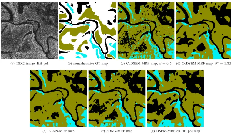
classifica-(a) TSX2 image, HH pol (b) nonexhaustive GT map (c) CoDSEM-MRF map, β = 0.5 (d) CoDSEM-MRF map, β∗= 1.324
(e) K-NN-MRF map (f) 2DNG-MRF map (g) DSEM-MRF on HH pol map
Fig. 2. (a) TSX2 image (750 × 750) in HH polarization, (b) nonexhaustive ground truth (GT) map (water ¥, wet soil¥, dry soil¥, outside GT ¤) and classification maps (water ¥, wet soil ¥, dry soil ¥): CoDSEM-MRF with (c) manually set β = 0.5 and (d) automatically estimated β∗ = 1.324, (e)
K-NN-MRF, (f) 2DNG-MRF and (g) DSEM-MRF on HH pol.
tion maps obtained by the benchmark 2D Nakagami-Gamma (2DNG) model [18] (Fig. 1(c)) and K-nearest neighbors (K-NN) method [34] (Fig. 1(d)). In order to perform a fair comparison among contextual methods, the above models were combined with the contextual MRF approach. The same MRF parameter estimation and energy minimization procedures as in CoDSEM-MRF were considered in these benchmark experiments as well. For the 2DNG model, the equivalent number of looks was set to L = 2.66, and for the K-NN model, K∗= 40 was estimated by cross-validation [34]. The
overall accuracies of these two benchmark approaches were 81.5% for 2DNG-MRF and 81.9% for K-NN-MRF on the dual-pol HH/VV TSX1 image. These accuracies were lower than the overall classification accuracy achieved by CoDSEM-MRF. K-NN-MRF had higher accuracy for the “wet soil” class, however this was achieved at the expense of accuracy for the “dry soil.” A visual comparison of the zoomed area in Fig. 1(h)-(l) confirms these comments.
The second test image TSX2 (see Fig. 2) was taken from the same dataset as TSX1. It employed the same learning image and, thus, the same set of copulas were selected. The overall classification accuracy obtained by CoDSEM-MRF was 92.4% with β∗ = 1.324. This accuracy is higher than
that reported for the TSX1 image, however, this increase is mostly due to non-exhaustive test map employed in this experiment, which did not contain much of the class transition regions where misclassified pixels may be visually spotted. The single channel DSEM-MRF classification on HH-pol
TABLE III
CLASSIFICATION ACCURACIES ON THE CONSIDERED TEST IMAGES:CLASS ACCURACIES,AVERAGE ACCURACIES,AND OVERALL ACCURACIES. Image Method Water Wet soil Dry soil Average Overall TSX1 CoDSEM-MRF 90.02% 82.56% 84.80% 85.79% 84.55% 2DNG-MRF 89.33% 82.12% 76.51% 82.78% 81.49% K-NN-MRF 87.15% 87.81% 71.45% 82.14% 81.95% DSEM-MRF VV 90.00% 69.93% 91.28% 83.74% 80.61% TSX2 CoDSEM-MRF, β∗ 92.48% 94.59% 85.16% 90.49% 92.41% CoDSEM-MRF, β 91.52% 89.31% 77.48% 86.11% 87.98% 2DNG-MRF 92.59% 89.33% 86.01% 89.31% 89.74% K-NN-MRF 90.21% 98.56% 78.91% 89.23% 92.61% DSEM-MRF HH 93.93% 83.50% 90.27% 90.23% 87.11% CSK1 DSEM-MRF 95.57% 92.22% 92.45% 93.41% 93.14% K-root-MRF 89.64% 87.78% 96.83% 91.53% 90.94%
image(Fig. 2(g)) provided the overall accuracy of 87.1%, which is about 5% less than that of CoDSEM-MRF. Again, we provide comparisons with benchmark 2DNG-MRF (Fig. 2(f)) and K-NN-MRF (Fig. 2(e)) classification approaches. Like in the TSX1 image test, here CoDSEM-MRF outperformed appreciably 2DNG-MRF (89.7% of overall accuracy). K-NN-MRF with 92.6%, however, reported about the same level of overall accuracy as CoDSEM-MRF. Here we make the same observation as for TSX1 image: K-NN-MRF performed better on “wet soil” and far worse on “dry soil”. We notice also
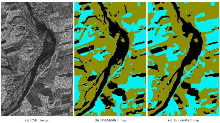
(a) CSK1 image (b) DSEM-MRF map (c) K-root-MRF map
Fig. 3. (a) CSK1 image (500 × 800) in HH polarization, and classification results (water ¥, wet soil¥, dry soil¥): (b) DSEM-MRF and (c) K-root-MRF classification maps.
that the average accuracy of K-NN-MRF is inferior to that of CoDSEM-MRF on both TSX1 and TSX2. Moreover, from the methodological point of view, CoDSEM is preferable to K-NN as it provides an explicit description of a statistical model for the data, whereas the latter operates as a “black box”.
A slight oversmoothing effect can be noticed in the results obtained by the developed method, see Fig. 2(d). Therefore, for the TSX2 image, we also show the classification map obtained by manually setting the MRF parameter β = 0.5 (Fig. 2(c)). One can see that the the spatial details are more precise at the expense of a noisier segmentation. The classification accuracies achieved with β = 0.5 (see Table III) are inferior to those obtained in the β∗ = 1.324 case. This suggests that,
at least for this dataset, a stronger regularization is overally more preferable.
The third experiment was conducted on a single-pol CSK1 image (see Fig. 3(a)). It also employed a non-exhaustive GT. The overall classification accuracy of DSEM-MRF (Fig. 3(b)) was 93.1% with β∗ = 1.566. We compare this with the
K-root-MRF contextual classification approach that is based on a K-root model [25] for each class-conditional statistics. The
K distribution is a well-known model for a possibly textured
SAR multilook single-channel intensity and K-root is the corresponding amplitude parametric pdf. Overall classification accuracy reported in this experiment (Fig. 3(c)) was equal to 90.9%. The improved performance of DSEM-MRF is due to more accurate pdf estimates by DSEM compared to K-root model.
The restriction of the DSEM dictionary DM to four models
compared to eight constituting the dictionary in [24] (see Sec.
III(a)) resulted in a negligible decrease in modeling accuracy. In other words, this restriction affected the classification accu-racy marginally, yet allowed a significant gain in calculation speed.
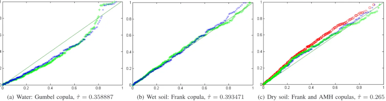
In addition, we want to demonstrate the accuracy of the Copula-DSEM joint pdf model directly. To do so we present the K-plots [47] of the sample HH-VV dependence and the dependence estimated by copulas (see Fig. 4) on the learning image for TSX1. K-plots is a tool for graphical goodness-of-fit presentations and its definition is recalled in Appendix B. The demonstrated copulas were automatically selected from the dictionary DM and one can see a good agreement between
observations and the model.
Let us now briefly compare the developed CoDSEM-MRF approach with the previously proposed copula-based method [21]. Firstly, the approach [21] is based on the use of the Ali-Mikhail-Haq (AMH) copula [31], which can model dependencies corresponding to Kendall’s correlation coeffi-cient τ ∈ [−0.1817, 0.3333]. On the employed TSX datasets we have observed empirical values ˆτwater ≈ 0.36, ˆτwet ≈
0.39, ˆτdry ≈ 0.27. Therefore, the AMH copula can be used
only for the dry soil class and its K-plot is presented in Fig. 4(c). However, even in this case, the goodness-of-fit provided by the automatically selected Frank copula is better. Thus, the use of dictionary-based copula selection approach is more accurate and constitutes a more flexible model with a wider range of applicability. Secondly, the use of the DSEM finite mixture estimation approach for marginal pdf estimation provides higher accuracy estimates than singular pdf models the use of which was suggested in [21], especially for HR
(a) Water: Gumbel copula, ˆτ = 0.358887 (b) Wet soil: Frank copula, ˆτ = 0.393471 (c) Dry soil: Frank and AMH copulas, ˆτ = 0.265 Fig. 4. K-plots display the graphical goodness-of-fit for copula models on the learning stage for TSX1 image. For the considered three classes the sample HH-VV dependences (+) are fitted by automatically selected copulas (×). The K-plot for the Ali-Mikhail-Haq (AMH) copula (o) is also presented for the dry soil class (c). The diagonal (–) represents the independency scenario.
Fig. 5. The sensitivity of CoDSEM-MRF classification accuracy to the size of the learning image. The class accuracies (water¤, wet soil◦, dry soil♦) and overall accuracies (solid line,x) are reported for TSX1 image. The initial learning image is 250 × 250 pixels.
SAR images [24].
It is well known, that the acquisition of the training sets required for the supervised classification is a very costly procedure. Therefore, the classification models are designed to be as robust as possible with respect to small learning sets. To evaluate this characteristic of the proposed algorithm, we present an experimental study (see Fig. 5) of the classification accuracy as a function of size of the employed training set. We start with the learning image of 250 × 250 pixels, and then iteratively reduce its size by a half at each step, i. e. by discarding 50% randomly selected training pixels for each the-matic class, untill 1/32 of the initial learning image is present. At each step we evaluate the class and overall accuracies of classification on TSX1. To make the accuracy estimates more consistent, the whole process was repeated three times and the averaged results are presented in Fig. 5. We observe that the algorithm behaves robustly till 1/8 (90 × 90 pixels) of the initial learning image is kept. When very strong subsampling rates (> 16) are applied, the wet area classification rate drops significantly. This is due to the fact that the histogram of wet soil lies “between” those of water and dry soil. Thus, when the training set becomes unrepresentatively small, a lot of wet soil pixels are misclassified as dry soil. This result suggests the capability of the developed algorithm to perform fairly good and consistently on small training sets, i.e. up to 100 × 100 training images for the considered dataset.
The most time consuming stages of the algorithm are the MRF and Energy minimization steps. Given the fairly low value K0 = 3, the DSEM step was very fast. The Copula
and MRF steps do not involve any intensive computation procedures. The experiments were conducted on a Core 2 Duo 1.83GHz, 1Gb RAM, WinXP system. With the number of iterations equal to 200, the β-estimation on a roughly 1000 × 1000 image took around 80 seconds. The average of 200 iterations required for convergence on MMD (Energy minimization step) took about 100 seconds. Thus about 200 seconds were required for the complete classification process of a 1000 × 1000 dual-pol image with three classes.
V. CONCLUSIONS
Contemporary satellite SAR missions, such as TerraSAR-X and COSMO-SkyMed, are capable of providing high resolu-tion imagery. In this paper, a novel supervised classificaresolu-tion algorithm for HR single channel and dual polarization satellite SAR imagery has been developed. It combines the Markov random field approach to Bayesian image classification and a finite mixture technique for probability density function estimation. Finite mixture modeling was done via dictionary-based stochastic expectation maximization for amplitude pdf estimation, which provides a high level of estimation accuracy for the algorithm [24]. These two concepts allowed us to formulate a classification algorithm for the case of single-channel SAR imagery. The second contribution of this paper is the introduction of a novel statistical approach based on a dictionary of copulas for the problem of dual polarization SAR image classification. This approach enables a new level of flexibility in modeling the joint distribution from marginal single-channel distributions, which results in higher classifica-tion accuracy. Together with Markov random fields and finite mixture approaches, these three statistical concepts ensure high flexibility and applicability of the developed method to dual-pol HR SAR image classification.
The proposed classification algorithm is supervised and semiautomatic (a few DSEM and MMD parameters have to be specified). The accuracy of the proposed algorithm was validated for water/wet soil/dry soil classification on two high resolution satellite SAR images (a dual-pol TerraSAR-X image
and a single-pol COSMO-SkyMed image). The experiments demonstrated a high level of accuracy on the experiment datasets and outperformed the considered parametric and non-parametric contextual benchmark algorithms.
Finally, we would like to point out several directions of further development of this work. First of all, a very inter-esting topic would be the generalization of the developed copula-based approach to multi-polarized imagery and its application to quad-pol TerraSAR-X imagery. The theory of copulas allows an extension of bivariate theory to multivariate cases, thus preserving the same copula types and parameter estimation techniques. However, contrary to the symmetric copulas approach considered here, which implied equal “con-tributions” of all marginal channels in the joint distribution, non-symmetric copulas would have to be considered for multi-polarization scenario. Another interesting direction of work is to explore the use of more efficient optimization approaches. A very promising candidate to replace MMD is an appropriate graph cut approach [48]. Such approaches yield very good approximations in the MAP segmentation problem and are known to be fast. The third direction of development lies in the specialization of this model to urban area classification, which is an important and relevant application of SAR classification. To this end, the contextual MRF model would also need to incorporate geometrical information.
APPENDIXA BIVARIATE COPULA THEORY
A bivariate copula is a function C : [0, 1]2→ [0, 1], which
satisfies the following properties:
1. both marginals are uniformly distributed on [0, 1];
2. for every u,v in [0, 1]: C(u, 0) = C(0, v) = 0, and
C(u, 1) = u, C(1, v) = v;
3. a 2-increasing property: ∀u1 6 u2, v1 6 v2 in [0, 1]:
C(u2, v2) − C(u1, v2) − C(u2, v1) + C(u1, v1) > 0.
The importance of copulas in statistics is explained by Sklar’s Theorem [31], which states the existence of a copula
C, that models the joint distribution function H of arbitrary
random variables X and Y with CDFs F and G:
H(x, y) = C(F (x), G(y)), (7) for all x, y in R. If, in addition, F and G are continuous, then
C is unique. Thus, copulas link joint distribution functions to
their one-dimensional marginals.
Given absolutely continuous random variables with pdfs
f (x) and g(y) and corresponding CDFs F (x) and G(y), the
pdf of the joint distribution h(x, y) corresponding to (7) is given by:
h(x, y) = f (x)g(y) ∂
2C
∂x∂y(F (x), G(y)), (8)
where ∂2C
∂x∂y(x, y) is pdf corresponding to the copula C(x, y).
An important family of copulas are Archimedean copulas, which have a simple analytical form and yet provide a wide variety of modeled dependence structures. An Archimedean copula is a bivariate copula C, defined as:
C(u1, u2) = φ−1(φ(u1) + φ(u2)),
where the generator function φ(u) is any function satisfying the following properties:
1. φ(u) is continuous on [0, 1];
2. φ(u) is decreasing, φ(1) = 0;
3. φ(u) is convex.
A common way of copula estimation is by using its con-nection with Kendall’s tau, which is a ranking correlation coefficient [31]. Kendall’s tau is a concordance-discordance measure between two independent realizations (X, Y ) and ( ˆX, ˆY ) from the same CDF H(x, y):
τ = Prob{(X − ˆX)(Y − ˆY ) > 0} −
Prob{(X − ˆX)(Y − ˆY ) < 0}.
Given realizations (xl, yl), l = 1, . . . , N , the empirical
esti-mator of Kendall’s tau is given by: ˆ τ = 4 N (N − 1) X i6=j I[xi6 xj]I[yi6 yj] − 1. (9)
By integrating in the definition of τ over the distribution of ( ˆX, ˆY ), we get the general relationship between Kendall’s τ
and the copula C associated with H(x, y), expressed by the following Lebesgue-Stieltjes integral:
τ + 1 = 4 1 Z 0 1 Z 0 C(u, v)dC(u, v), (10) In the specific case of Archimedean copulas, the relationship is expressed in terms of generator function φ(t):
τ = 1 + 4 1 Z 0 φ(t) φ0(t)dt. (11)
By plugging the empirical estimate ˆτ in place of τ in
Eq. (10) or (11), we get parameter estimates ˆθ (see Table II).
APPENDIXB
GRAPHICAL GOODNESS-OF-FIT BYK-PLOTS A K-plot (from Kendall-plot) [47] is a rank based graph-ical tool developed for visualization of dependence structure between two random variables X and Y . This technique is based on plotting the pairs (Wi:N, H(i)) for i = 1, . . . , N :
• H(i) are defined as H(1) 6 H(2) 6 · · · 6 H(N ), i.e. the order statistics of quantities
Hi=
1
N − 1#{j 6= i : xi6 xj, yi6 yj}. • Wi:N represents the expectation of the ith order statistic
in a random sample of size N from the distribution
K0(ω) = Prob{H(X, Y ) 6 ω} of the Hi under the null
hypothesis of independency. It writes [47]:
Wi:N = N µ N − 1 i − 1 ¶ × Z 1 0 ω {K0(ω)}i−1{1 − K0(ω)}N −idK0(ω), (12) where K0(ω) = ω − ω log ω.
In order to compare this sample dependence representation with the one provided by a given copula we need to find the form of Kθ(ω) = Prob{Cθ(U, V ) 6 ω} specific to this copula,
where U ∼ F (X), V ∼ G(Y ). It can be found as [49]
Kθ(ω) = ω −φθ(ω)
φ0 θ(ω)
, ω ∈ (0, 1),
for an Archimedean copula with generator φθ(·). Replacing
then K0(ω) by Kθ(ω) in (12) we can also draw a plot
(cWi:N, H(i)) that corresponds to a given copula and where θ
is estimated via Kendall’s tau (see Appendix A). Finally, the generators for Gumbel and Frank copulas are given by [31]:
φGumbel(ω) = (− ln ω)θ, φFrank(ω) = − lne
−θω− 1
e−θ− 1 .
ACKNOWLEDGMENT
The authors would like to thank the Italian Space Agency for providing the COSMO-SkyMed (CSK°) im-R
age of Piemonte (COSMO-SkyMed Product - c°ASI
-Agenzia Spaziale Italiana - 2008. All Rights Reserved). The TerraSAR-X image of Sanchagang was taken from
http://www.infoterra.de/, where it is available for free testing
( c°Infoterra GmbH, 2008). The authors would also like to
thank the anonymous reviewers for their helpful and construc-tive comments.
REFERENCES
[1] C. Oliver and S. Quegan, Understanding Synthetic Aperture Radar
Images, 2nd ed. NC, USA: SciTech, Raleigh, 2004.
[2] J.-S. Lee and E. Pottier, Polarimetric Radar Imaging: From Basics to
Applications. New York: CRC Press, 2009.
[3] J.-S. Lee, M. R. Grunes, and R. Kwok, “Classification of multilook polarimetric SAR imagery based on complex Wishart distribution,” Int.
J. Remote Sensing, vol. 15, no. 11, pp. 2299–2311, 1994.
[4] J.-M. Beaulieu and R. Touzi, “Segmentation of textured polarimetric SAR scenes by likelihood approximation,” IEEE Trans. Geosci. Remote
Sens., vol. 42, no. 10, pp. 2063–2072, 2004.
[5] A. C. Frery, C. C. Freitas, and A. H. Correia, “Classifying multifre-quency fully polarimetric imagery with multiple sources of statistical evidence and contextual information,” IEEE Trans. Geosci. Remote
Sens., vol. 45, no. 10, pp. 3098–3109, 2007.
[6] A. P. Doulgeris, S. N. Anfinsen, and T. Eltoft, “Classification with a non-Gaussian model for PolSAR data,” IEEE Trans. Geosci. Remote
Sens., vol. 46, no. 10, pp. 2999–3009, 2008.
[7] L. Bombrun, G. Vasile, M. Gay, and F. Totir, “Hierarchical seg-mentation of polarimetric SAR images using heterogeneous clut-ter models,” IEEE Trans. Geosci. Remote Sens., 2010, (to appear). DOI:10.1109/TGRS.2010.2060730.
[8] Y. Ito and S. Omatu, “Polarimetric SAR data classification using competitive neural networks,” Int. J. Remote Sensing, vol. 19, no. 14, pp. 2665–2684, 1998.
[9] K. S. Chen, W. P. Huang, D. H. Tsay, and F. Amar, “Classification of multifrequency polarimetric SAR imagery using a dynamic learning neural network,” IEEE Trans. Geosci. Remote Sens., vol. 34, no. 3, pp. 814–820, 1996.
[10] C. Lardeux, P.-L. Frison, C. Tison, J.-C. Souyris, B. Stoll, B. Fruneau, and J.-P. Rudant, “Support vector machine for multifrequency SAR polarimetric data classification,” IEEE Trans. Geosci. Remote Sens., vol. 47, no. 12, pp. 4143–4152, 2009.
[11] C. T. Chen, K. S. Chen, and J.-S. Lee, “The use of fully polarimetric information for the fuzzy neural classification of SAR images,” IEEE
Trans. Geosci. Remote Sens., vol. 41, no. 9, pp. 2089–2100, 2003. [12] P. R. Kersten, J.-S. Lee, and T. L. Ainsworth, “Unsupervised
classi-fication of polarimetric synthetic aperture radar images using fuzzy clustering and EM clustering,” IEEE Trans. Geosci. Remote Sens., vol. 43, no. 3, pp. 519–527, 2005.
[13] J. Morio, F. Goudail, X. Dupuis, P. Dubois-Fernandez, and P. Refregier, “Polarimetric and interferometric SAR image partition into statistically homogeneous regions based on the minimization of the stochastic complexity,” IEEE Trans. Geosci. Remote Sens., vol. 45, no. 12, pp. 3599–3609, 2007.
[14] K. Ersahin, I. Cumming, and R. Ward, “Segmentation and classification of polarimetric SAR data using spectral graph partitioning,” IEEE Trans.
Geosci. Remote Sens., vol. 48, no. 1, pp. 164–174, 2010.
[15] G. D. De Grandi, J. S. Lee, and D. L. Schuler, “Target detection and texture segmentation in polarimetric SAR images using a wavelet frame: Theoretical aspects,” IEEE Trans. Geosci. Remote Sens., vol. 45, no. 11, pp. 3437–3453, 2007.
[16] S. R. Cloude and E. Pottier, “An entropy based classification scheme for land applications of polarimetric SAR,” IEEE Trans. Geosci. Remote
Sens., vol. 35, no. 1, pp. 68–78, 1997.
[17] J.-S. Lee, M. R. Grunes, E. Pottier, and L. Ferro-Famil, “Unsupervised terrain classification preserving polarimetric scattering characteristics,”
IEEE Trans. Geosci. Remote Sens., vol. 42, no. 4, pp. 722–731, 2004. [18] J.-S. Lee, K. W. Hoppel, S. A. Mango, and A. R. Miller, “Intensity
and phase statistics of multilook polarimetric and interferometric SAR imagery,” IEEE Trans. Geosci. Remote Sens., vol. 32, no. 5, pp. 1017– 1028, 1994.
[19] S. H. Yueh, J. A. Kong, J. K. Jao, R. T. Shin, and L. M. Novak, “K-distribution and polarimetric terrain radar clutter,” J. Electromagn. Waves
Applicat., vol. 3, pp. 747–768, 1989.
[20] C. C. Freitas, A. C. Frery, and A. H. Correia, “The polarimetric G distribution for SAR data analysis,” Environmetrics, vol. 16, no. 1, pp. 13–31, 2005.
[21] G. Mercier and P.-L. Frison, “Statistical characterization of the Sinclair matrix: Application to polarimetric image segmentation,” in Proceedings
of IGARSS, Cape Town, South Africa, 2009, pp. III–717–III–720. [22] Z. Kato, J. Zerubia, and M. Berthod, “Unsupervised parallel image
classification using Markovian models,” Pattern Recognit., vol. 32, no. 4, pp. 591–604, 1999.
[23] G. Moser, S. Serpico, and J. Zerubia, “Dictionary-based Stochastic Ex-pectation Maximization for SAR amplitude probability density function estimation,” IEEE Trans. Geosci. Remote Sens., vol. 44, no. 1, pp. 188– 199, 2006.
[24] V. Krylov, G. Moser, S. B. Serpico, and J. Zerubia, “Enhanced dictionary-based SAR amplitude distribution estimation and its valida-tion with very high-resoluvalida-tion data,” IEEE Geosci. Remote Sens. Lett., vol. 8, no. 1, pp. 148–152, 2011.
[25] E. Jakeman and P. N. Pusey, “A model for non-Rayleigh sea echo,” IEEE
Trans. Antennas Propagat., vol. 24, pp. 806–814, 1976.
[26] Y. Delignon, A. Marzouki, and W. Pieczynski, “Estimation of general-ized mixtures and its application in image segmentation,” IEEE Trans.
Image Process., vol. 6, no. 10, pp. 1364–1375, 1997.
[27] C. Tison, J.-M. Nicolas, F. Tupin, and H. Maitre, “A new statistical model for Markovian classification of urban areas in high-resolution SAR images,” IEEE Trans. Geosci. Remote Sens., vol. 42, no. 10, pp. 2046–2057, 2004.
[28] E. E. Kuruoglu and J. Zerubia, “Modelling SAR images with a gen-eralization of the Rayleigh distribution,” IEEE Trans. Image Process., vol. 13, no. 4, pp. 527–533, 2004.
[29] G. Moser, J. Zerubia, and S. B. Serpico, “SAR amplitude probability density function estimation based on a generalized Gaussian model,”
IEEE Trans. Image Process., vol. 15, no. 6, pp. 1429–1442, 2006. [30] H.-C. Li, W. Hong, and Y.-R. Wu, “Generalized Gamma distribution
with MoLC estimation for statistical modeling of SAR images,” in
Proceedings of APSAR, Huangshan, China, 2007, pp. 525–528. [31] R. B. Nelsen, An Introduction to Copulas, 2nd ed. New-York: Springer,
2006.
[32] G. Mercier, S. Derrode, W. Pieczynski, J.-M. Nicolas, A. Joannic-Chardin, and J. Inglada, “Copula-based stochastic kernels for abrupt change detection,” in Proceedings of IGARSS, Denver, USA, 2006, pp. 204–207.
[33] G. Mercier, G. Moser, and S. Serpico, “Conditional copulas for change detection in heterogeneous remote sensing images,” IEEE Trans. Geosci.
Remote Sens., vol. 46, no. 5, pp. 1428–1441, 2008.
[34] C. M. Bishop, Pattern Recognition and Machine Learning. New-York: Springer, 2006.
[35] V. Krylov and J. Zerubia, “High resolution SAR image classification,” INRIA, Research Report 7108, 2009. [Online]. Available: http://hal.archives-ouvertes.fr/docs/00/44/81/40/PDF/RR-7108.pdf
[36] J. Besag, “On the statistical analysis of dirty pictures,” J. Royal Stat.