A Mathematical Approach Estimating Source and Sink Functioning of Competing Organs

HAL Id: inria-00121569

https://hal.inria.fr/inria-00121569

Submitted on 24 Jan 2007

HAL is a multi-disciplinary open access

archive for the deposit and dissemination of sci-entific research documents, whether they are pub-lished or not. The documents may come from teaching and research institutions in France or abroad, or from public or private research centers.

L’archive ouverte pluridisciplinaire HAL, est destinée au dépôt et à la diffusion de documents scientifiques de niveau recherche, publiés ou non, émanant des établissements d’enseignement et de recherche français ou étrangers, des laboratoires publics ou privés.

Functioning of Competing Organs

M.Z. Kang, Philippe de Reffye

To cite this version:

M.Z. Kang, Philippe de Reffye. A Mathematical Approach Estimating Source and Sink Functioning of Competing Organs. Proceedings of the Frontis Workshop on Functional -structural Plant Modelling in Crop Production, Wageningen University and Research Centre, Mar 2006, Wageningen / Netherlands, Netherlands. pp.65-75. �inria-00121569�

page-odd J. Vos, L.F.M. Marcelis, P.H.B. de Visser, P.C. Struik and J.B. Evers (eds.), Functional-Structural Plant Modelling in Crop Production, xx-xx.

© 2007 Springer. Printed in the Netherlands.

CHAPTER 6

A MATHEMATICAL APPROACH ESTIMATING

SOURCE AND SINK FUNCTIONING OF

COMPETING ORGANS

MENGZHEN KANG

AND PHILIPPE DE REFFYE

1 Capital Normal University, BeiJing, China 2 DigiPlante, INRIA, Rocquencourt, France

3 AMAP, CIRAD, Montpellier, France

4 LIAMA, Institute of Automation, CAS, BeiJing, China

Abstract. Plant growth and development depend on both organogenesis and photosynthesis.

Organogenesis sets in place various organs (leaves, internodes, fruits, roots) that have their own sinks. The sum of these sinks corresponds to the plant demand. Photosynthesis of the leaves provides the biomass supply (source) that is to be shared among the organs according to their sink strength.

Here we present a mathematical model – GreenLab – that describes dynamically plant architecture in a resource-dependent way. The source and sink functions of the various organs control the biomass acquisition and partitioning during plant development and growth, giving the sizes and weights of organs according to their position in the plant architecture. Non-linear least-square method was used to estimate the numerical values of (hidden) parameters that control the organ sink variation and leaf functioning. Through simultaneous fitting of data from several developmental stages (multi-fitting), plant growth could be described satisfactorily with just a few parameters. Examples of application on cotton and maize are shown in this article.

INTRODUCTION

In this chapter we will use these terms: process-based model (PBM), structural plant model (SPM) and functional-structural plant model (FSPM). We will focus on our main subject: to make proper estimation on both the biomass production and the biomass partitioning during the plant growth process, by using the plant architecture as a support. Until now the solution of this problem is not fulfilled for several reasons. In SPMs, plant architectures are not linked to biomass production and partitioning; the dimensions of organs are given directly, either from measurement

or from predefined data. PBMs handle the sink and source relationships, but they do not integrate plant architecture, although leaf area index (LAI) is an important parameter. Moreover, prediction of leaf area is still a weak point in PBMs (Marcelis et al. 1998). FSPMs seem to be the ideal solution for the problem posed above, but model application is often constrained by the simulation software, which is of high complexity and bug-sensitive. Lack of dynamic equations describing both the development and growth process in most FSPMs gives difficulty in getting derivatives for optimization methods. The computational cost is high (Sievänen et al. 2000), so that the use of the classical heuristics for estimation, such as genetic algorithms, will take too much computation time to be realistic.

NEW RELEVANT CHOICES FOR FSPMS

We consider here building a robust mathematical plant growth model, GreenLab, which belongs to the FSPM family although its philosophy is close to PBMs. One of the differences from PBMs is that the processes of sink and source are modelled at the level of individual organs, each having its age according to the position inside plant structure.

Several levels of complexity are currently involved in GreenLab: (1) the deterministic case (Yan et al. 2004), where the plant development is independent of the plant growth (case of this chapter); (2) the stochastic case (Kang 2003), where bud growth, death and branching pattern occur with certain probabilities, thus both number of organs and biomass production are stochastic; and (3) the feedback case (Rostand-Mathieu 2006), where the plant development depends on the relationship between biomass supply and demand. Here we focus only on the first deterministic case. The basic concepts are common for all approaches. The environment factor is not considered here, although it is dealt with in the GreenLab model, as in Wu (2006). We present some examples of model calibration on cultivated plants.

About plant development

Automaton (deterministic or stochastic) was specially designed by Zhao et al. (2001) to simulate different kinds of the architectural models as defined in Hallé et al. (1978). It simulates the occupancy and transition laws that control organ differentiation. The notion physiological age (PA) was introduced to distinguish different kinds of axis. An axillary bud has a PA not less than that of the axis from which it originates. Let PA=1 for the main axis, the maximum PA of plants is generally less than 5. Besides, each part of the plant (organs, branches or the plant itself) has a chronological age (CA), meaning the number of growth cycles (GCs) it has passed since its appearance. Each GC corresponds to the time duration for creating macroscopically a new growth unit (GU) in the axis, including either one (for crops) or several (for trees) phytomers. The apical bud of an axis can transform into another PA after certain GCs.

The number of organs produced by the automaton can be computed recurrently based on a high level of factorization thanks to the notions PA and CA (De Reffye

and Cournède 2005). This recurrent formula speeds up dramatically the computation and visualization by avoiding the common use of parallel time-consuming simulations. Let up be the number of organs of type o per GU for a given PA p, and

cp,k be the number of branches of PA k on the GU of PA p. In the case that the axis

has not transformed into another PA, in a plant of maximum PA m, the number of organs o in a structure of PA p and CA t can be computed with Equation (1):

[ ] [ ]

_∑∑

[ ]

[ ] [

] [ ] [

] [ ] [

]

means number of organs o of PA k in the structure of PA p. npk(p>k) is zero

according to the rule of PA. The computation begins with [Nm], which is number of

organs o in a single stem structure, and finishes with [N1], for the plant itself. To

distinguish organs of different PA, CA and type, we note np( tj, )

o as the number of organs of type ‘o’, CA ‘j’ and PA ‘p’ in the plant of GC t.

About plant growth

The plant yields are described as a result of the dynamic growth process where each organ plays its role as source and/or sink. The source organs are the leaves, and the

seed in the first GCs; the sink organs are leaves, internode (pith and cambium), fruits and roots during their expansions. Each source organ fills directly a common pool of biomass reserve while each sink organ withdraws biomass according to its relative sink strength.

The organs may have different expansion schedules because the conditions of the biomass production and partitioning change at each step of growth. For example, appearance of fruits may disrupt the growth of the vegetative organs because of their stronger sink strength. However, we assume the sink functions are the same for a given kind of organ, because growth of individual organs of the same kind follows similar patterns in a plant when there is nodisruption. Sink functions for pith and cambium must be distinguished because they belong to primary and secondary growth separately. Moreover, the blade and petiole in a leaf may follow different growth pattern. In total there are no more than seven sink functions.

Each kind of organ o (of PA p) has a relative sink value, Pop, standing for the

ability of competing biomass. Set that of the blade in the main stem (PA=1) to 1 as the reference value. Besides, the sink strength of an organ can vary during its expansion. For an organ o of CA j and PA p, its sink strength, pop(j), is finally:

o b o a o T j o o o o o o p o p o T j T j j g j g j g j f where T j T j j f P j p o o o / ) 5 . 0 ( ) 5 . 0 ( ) ( , ) ( / ) ( ) ( ) ( 0 ) 1 ( ) ( ) ( 1 1 1 − − = = − − + = ⎩ ⎨ ⎧ > ≤ ≤ =

∑

In Equation (2), To is the expansion duration of an organ o, fo(j) is a normalized

function that describes the sink variation of an organ during growth. This is a discrete extension of Beta law because its shape is very flexible. The original variable of Beta law is replaced with (j-0.5/To) since its range must be (0,1). ao and

bo are the parameters of the function go, that give the pattern of expansion. The

observable values, To, can evolve during the plant growth, but the parameters, ao and

bo, that control the shape of the functions, are supposed to be constant since the

expansion pattern of organ o remains almost the same. Similar assumptions can be found in SPM about the leaf elongation, with a scale factor depending on the organ position (Fournier and Andrieu 1999).

The plant demand at GC t, D(t), is defined as the sum of sinks of all growing organs. It can be written as in Equation (3):

∑∑∑

Biomass production is computed with the Beer-Lambert law, where LAI is computed from all functioning leaves, as in Equation (4):

[

]

P _{k LAI t whereLAI t n jt S jt S}

k r S t E t Q 1 exp( ()), () ( , ) ( , )/ . ) ( ) ( 1 1

∑∑

Here ta is the functioning duration of leaves in GC, another observable parameter of the model. Sp_(j,t)

.is the surface area of a leaf of PA p and CA j at plant age t,

computed from its weight. Sp is the projection area of the plant, linked to the density

of planting. E(t) is a climate factor in GC t. The parameter r is a resistance term that resides in the leaves, and k is the light-extinction coefficient (Guo et al. 2006).

The portion of biomass assimilation Δqop(j,t), flown into the organ o of PA p and

CA j at plant age t, depends on 3 factors: its current sink strength as in Equation (2), the global plant demand as in Equation (3), and the biomass supply available into the plant architecture at the age n as in Equation (4):

) ( / ) ( ). , ( ) , (jt p j t Qt Dt q p o p o = Δ (5)

The weight of the organ, q, is the accumulated value of the Δq since it was created. Since the ratio Q/D varies during plant growth, thus the weights of the individual organs keep the memory of the evolution of this ratio.

The size of an organ depends on its weight and on allometric factors. For leaves, the blade thickness is an important factor to deduce the surface area from the weight. Most often the ratio between the blade weight and surface is roughly constant throughout the expansion period. For internode and petiole we consider a cylinder shape with length l, surface section s and volume v (thus l.s=v). On the other hand, there is an allometric relationship between l, s and q, as in Equation (6):

β

q b s

l/ = . (6)

The parameters b and β can be assessed with experimental data. Notice that q=v.d, d being the vegetative density of pith or petiole, from the weight we can get the length and diameter.

Two kinds of growth can coexist in internodes: the primary growth concerning the pith, which lasts several GCs until the length of the internode is stable, and the secondary growth concerning the cambium activity, which does not stop. In each GC a new layer of cambium is laid down along the stem. This layer is supposed to have a constant sink Pc without expansion and to have a uniform biomass linear

repartition all along the stem. The internode diameter is the result of both mechanisms.

With the initial biomass Q0, the size and weight of all organs can be computed

cycle by cycle. Eventually, one can build the plant architecture for visualization or for processing interactions with the environment (light interception, plant competition).

Calibration of the GreenLab model on real plants under a certain environment

To fit the model to certain real plant data, the parameters must be estimated. Parameters for automaton can be deduced from plant development. But the parameters that control the sink (Po, ao, bo) and source (r, k) functions generally can

not be assessed directly, so they are hidden. The thermal time of a GC can be defined according to the leaf appearance rate. If no information is available about the climate, the value of E is supposed to be constant. Slight variations of E usually have no important effect compared to constant climate, because they are smoothed by the successive steps of organ expansion.

The hidden parameters are to be estimated from the observed weights (and sizes) of the organs with a generalized least-square method (Press et al. 1992). Advantages of this method are that it provides rapid convergence and the standard error linked to the parameter values indicating the accuracy of the solution. The number of measured data must be larger than the number of hidden parameters. Fitting can be done on a single architecture (single fitting), or more accurately, on several stages of growth to follow the trajectory of the dynamical process (multi-fitting). In both cases all the data are fit simultaneously by the same parameter set. This differs from the SPM model, where fitting is done directly and only on the size of organs according to their locations on the plant. In the GreenLab model, the organ weights and sizes are the support to find the source and sink dynamics during the growth process.

Here we present two examples with only a single stem to explain what can be the target data and model parameters. Such simple architectures allow complete measurement and it is the most favourable case for assessing the value of the model.

Case of a leafy axis: a complete study on pruned cotton plant

Experiments on pruned cotton plant have been undertaken in CIRAD (1998) and CAU (2000) (De Reffye et al. 1999). No data on climate are available, so we set E(t) =1. The plant architecture is a single stem (branches removed) consisting of similar kinds of phytomers (internode + leaf). From phytomer rank 1 to 8, the leaf functioning duration increases from 6 to 13 GCs. After rank 8 it is stabilized.

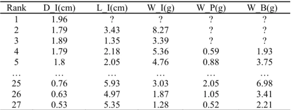
The leaf thickness is assessed to be 0.032 cm, the allometry parameters of the pith computed from the tip of the stem are b =64, β = 0.02. But those of the first internode are different. The expansion duration of the pith is set to the same values as that of the leaf of the same phytomer rank. Secondary growth exists for the internodes. We chose a cotton stem with 27 phytomers. At the bottom of the stem are some missing data because some leaves died and the first internode was not fully measured. Table 1 shows all the data that have to be fit by the corresponding output of the GreenLab model.

Table 1. The target data of a single-stem cotton plant: diameter, length and weight of the

internode, weight of petiole, and weight of blades of 27 phytomers

Rank D_I(cm) L_I(cm) W_I(g) W_P(g) W_B(g)

1 1.96 ? ? ? ? 2 1.79 3.43 8.27 ? ? 3 1.89 1.35 3.39 ? ? 4 1.79 2.18 5.36 0.59 1.93 5 1.8 2.05 4.76 0.88 3.75 … … … … … … 25 0.76 5.93 3.03 2.05 6.98 26 0.63 4.97 1.87 1.05 3.41 27 0.53 5.35 1.28 0.52 2.21 The GLSQM gives both parameter values and their standard deviation (x and ∆x). With the results in Table 2, the internode sink variation is J-shaped while the leaf one is bell-shaped.

Table 2. Hidden parameters for sink functions

Sink strength Sink variation parameters Type of organ Po ∆Po ao ∆ao bo ∆bo Leaf blade 1 - 3.7 0.2 7.3 0.3 Leaf petiole 0.311 0.011 3.7 0.2 7.3 0.3 Pith 0.038 0.002 0.46 0.1 1.54 0.2 Cambium 0.031 0.001 - - - -

Other estimated parameters are: seed biomass Q0= 1.2 (g), ∆Qo = 0.03. This value is used to build the first phytomer (epicotyle and cotyledon). Blade resistance

r= 39.6, ∆r= 2.2; coefficient of Beer Law: k = 0.61, ∆k = 0.06. It is interesting that

the GLSQM is able to extract the effect of light interception on the growth process. The model fits nicely the cotton plant architecture. However, as it is a single fitting, it is hard to know whether the parameters found are stable during dynamic growth.

0 10 20 30 40 1 5 9 13 17 21 Bl a d e fr e s h w e ig h t (g ) 0 100 200 300 400 5 15 25 35 0 200 400 600 800 1 5 9 13 17 21 Phytom er rank C ob f re s h w e ight ( g ) 0 200 400 600 800 5 15 25 35 Grow th cycle

Figure 1. Fresh weight of organs at individual level (left) and at compartment level (right) of

maize at six growth stages, for model output (lines) and measured data (symbols: ◇ -GC 8, ◆ - GC 12,○ - GC 16, ● - GC 21, - GC 27, ▲- GC 30) 0 5 10 15 20 25 1 5 9 13 17 21 Sh e a th fr e s h w e ig ht ( g ) 0 50 100 150 200 250 5 15 25 35 0 20 40 60 80 1 5 9 13 17 21 Int e rnode fr e s h w e ight ( g ) 0 150 300 450 600 5 15 25 35

Case of multi-fitting for growing plants with fruits: example of maize

In CAU, experiments have been undertaken on maize (Guo et al. 2006). The measurements have been carried out destructively on several stages of growth (GC 8, 12, 16, 21, 27, 30). The maize has 21 phytomers for this Chinese cultivar.

The architecture began with phytomers of short internodes and ended with the tassel, while the growth continued until GC 33. The parameter E here is chosen to be the average potential transpiration.

Results of fitting on six stages of growth. Figure 1 shows that the GreenLab model

works well. Here we can be reasonably sure that a same set of parameters controls the growth process, because the trajectory of the dynamical process is captured for the 6 stages. Here 12 parameters of source and sink functions control 381 data points. The accuracy of the parameters of sink function is necessarily less for the cob than for the leaf, because there is only one cob but twenty leaves on the plants.

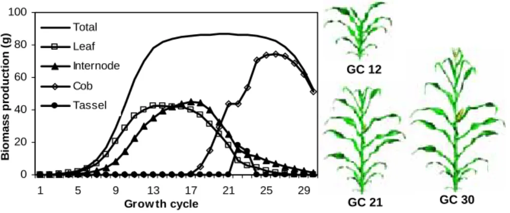
Simulating plant growth at each GC. Once the hidden parameters are estimated, the

problem of biomass production and biomass partitioning is solved as well. The model gives the amount of biomass fabricated by the plant at each stage of growth and how it is shared; see Figure 2. It is obvious that the cob was a big sink that inhibited the growth of vegetative organs. The plant architectures at some stages are displayed in Figure 2. The shape of organs comes from digitalization and their sizes are related to their weights thanks to their allometric rules.

0 20 40 60 80 100 1 5 9 13 17 21 25 29 Grow th cycle B io m a s s p rod uc ti on ( g ) Total Leaf Internode Cob Tassel

Figure 2. Modelled biomass production and partitioning at each cycle and 3D plant geometry

at three stages (Guo et al. 2006)

CONCLUSION

GreenLab has shown to be a good framework for modelling cultivated plants, like on other plants as wheat (Zhan et al. 2000), tomato (Dong 2006), sunflower (Yan et al. 2004) and chrysanthemum (Kang et al. in press).A main result is that the hidden

GC 12

functional parameters can be considered constant during the growth at a given environmental condition (Guo et al. 2006). These parameters are thus supposed to be endogenous for their characterization of the plant functioning.

The number of parameters is low (about 12) compared to the number of target data (can be >1000). However, since the number of parameters is fixed even if more plant data are fit simultaneously, here the over-fitting problem, which can often happen in training a neural network, does not exist. The sizes of organs along the stem are controlled by the organogenesis and sink–source functions. Detailed measurements at more stages help in calibrating the model to reproduce the dynamic growth history. However, sparse data, like weight of organs at compartment level or weight of individual organs, at just several phytomer ranks, are acceptable if one has enough knowledge of that plant. This will ameliorate the measurement efficiency.

With formulae giving number, size and weight of organs based on several assumptions, most of which are listed in Equations (1) to (6), computing a big plant (e.g., a tree of 40 years old and maximum branching order 3) takes only several seconds in DigiPlante software (Cournède and De Reffye 2005). This facilitates the application of optimization methods, as done for irrigation problems and sink-strength optimization (Lin 2006).

The model computes the biomass production and partitioning without physiological considerations. If the fitting is satisfactory, one set of constant parameters for the source and sink functions is enough to describe the dynamic growth process. If not, the differences between the prediction and the observations can help to better understand a possible physiological process of functioning. In case that the environment changes, functional parameters may change: for example, shadow conditions will generally increase the sink of the internode and its lengthening, and decrease the leaf thickness (Dong 2006). Nevertheless, another set of parameters devoted to a new condition controls pretty well the plant growth. Thus instead of being constant values, some parameters will be simple functions of environmental parameters. Experiments under different environmental conditions are needed to reveal the change of parameters. Eventually this allows undertaking optimization of the yield in various environmental conditions.

The results obtained on single-stem plants are to be generalized to plants with branching patterns (herbaceous, shrubs, trees). In addition to the plant structure complexity, the main theoretical problem occurring is how to take into account the interaction between growth and development, as done in Rostand-Mathieu (2006). For the functioning of the automaton that controls the plant development a key role is played by the biomass reserve, either stochastic or deterministic. Such studies are carrying out in China (LIAMA; CAU), France (ECP; INRIA) and the Netherlands (Wageningen University). Software that runs a full GreenLab model has been developed in C++: AMAPSim (Barczi et al. 1997), DigiPlante (Cournède and De Reffye 2005) in France, and in Scilab, an open-source software package by Kang et al. (www.greenscilab.org) in China.

ACKNOWLEDGEMENTS

We thank the anonymous reviewers. This work is supported in part by LIAMA, INRIA, CAU, ECP, CIRAD, WUR, Natural Science Foundation of China (#60073007), and China 863 Program (#2002AA241221) and (#2003AA209020).

REFERENCES

Barczi, J.F., De Reffye, P. and Caraglio, Y., 1997. Essai sur l’identification et la mise en oeuvre des paramètres nécessaires à la simulation d’une architecture végétale: le logiciel AMAPsim. In: Bouchon, J., De Reffye, P. and Barthélémy, D. eds. Modelisation et simulation de l'architecture des

végétaux. Institut National de la Recherche Agronomique, Paris, 255-423.

Cournède, P.H. and De Reffye, P., 2005. GreenLab: a dynamical model of plant growth for environmental applications. ERCIM News, 61, 41-41.

De Reffye, P., Blaise, F., Chemouny, S., et al., 1999. Calibration of a hydraulic architecture-based growth model of cotton plants. Agronomie, 19 (3/4), 265-280.

De Reffye, P. and Cournède, P.H., 2005. A powerful factorisation method to compute plant growth and architecture, applications in agronomy and computer graphics. In: 1st Open International Conference

on Modeling and Simulation (Oicms), June 12-15, 2005, ISIMA/Blaise Pascal University.

ISIMA/Blaise Pascal University. [http://www.isima.fr/oicms/pdf/I-1.pdf]

Dong, Q.X., 2006. Structural-functional simulation of crop growth combined with accurate radiation

transfer model-a case study on greenhouse tomato plant. China Agricultural University, Beijing.

PhD thesis China Agricultural University

Fournier, C. and Andrieu, B., 1999. ADEL-maize: an L-system based model for the integration of growth processes from the organ to the canopy: application to regulation of morphogenesis by light availability. Agronomie, 19 (3/4), 313-327.

Guo, Y., Ma, Y.T., Zhan, Z.G., et al., 2006. Parameter optimization and field validation of the structural-functional model GREENLAB for maize. Annals of Botany, 97 (2), 217-230.

Hallé, F., Oldeman, R.A.A. and Tomlinson, P.B., 1978. Tropical trees and forests: an architectural

analysis. Springer-Verlag, Berlin.

Kang, M.Z., 2003. Functional and structural stochastic plant modeling based on substructures. Chinese Academy of Sciences, Beijing. PhD thesis Chinese Academy of Sciences

Kang, M.Z., Heuvelink, E. and De Reffye, P., in press. Building virtual chrysanthemum based on sink-source relationships: preliminary results. Acta Horticulturae.

Marcelis, L.F.M., Heuvelink, E. and Goudriaan, J., 1998. Modelling biomass production and yield of horticultural crops: a review. Scientia Horticulturae, 74 (1/2), 83-111.

Press, W.H., Flannery, B.P., Teukolsky, S.A., et al., 1992. General linear least squares. In: Press, W.H., Teukolsky, S.A. and Vetterling, W.T. eds. Numerical recipes in FORTRAN: the art of scientific

computing. Cambridge University Press, Cambridge, 665-674. [http://library.lanl.gov/numerical/

bookfpdf/f15-4.pdf]

Rostand-Mathieu, A., 2006. Essai sur la modélisation des interactions entre la croissance et le

développement d'une plante: cas du modèle GreenLab. Ecole Centrale de Paris, Paris. PhD Thesis

Ecole Centrale de Paris

Sievänen, R., Nikinmaa, E., Nygren, P., et al., 2000. Components of functional-structural tree models.

Annals of Forest Science, 57, 399-412.

Wu, L., 2006. Variational methods applied to plant functional-structural dynamics: parameters

identification, control and data assimilation. Université Joseph Fourier, Grenoble. PhD Thesis

l’Université Joseph Fourier-Grenoble I

Yan, H., Kang, M., De Reffye, P., et al., 2004. A dynamic, architectural plant model simulating resource-dependent growth. Annals of Botany, 93 (5), 591-602.

Zhan, Z.G., Wang, Y.M., De Reffye, P., et al., 2000. Architectural modeling of wheat growth and validation study. In: Proceedings ASAE annual international meeting, July 9-12, 2000, Milwaukee,

Zhao, X., De Reffye, P., Xiong, F.L., et al., 2001. Dual-scale automaton model for virtual plant development. Chinese Journal of Computers, 24 (6), 608-615.