HAL Id: hal-01762446
https://hal.inria.fr/hal-01762446
Submitted on 10 Apr 2018
HAL is a multi-disciplinary open access
archive for the deposit and dissemination of
sci-entific research documents, whether they are
pub-lished or not. The documents may come from
teaching and research institutions in France or
abroad, or from public or private research centers.
L’archive ouverte pluridisciplinaire HAL, est
destinée au dépôt et à la diffusion de documents
scientifiques de niveau recherche, publiés ou non,
émanant des établissements d’enseignement et de
recherche français ou étrangers, des laboratoires
publics ou privés.
End-to-End Learning of Polygons for Remote Sensing
Image Classification
Nicolas Girard, Yuliya Tarabalka
To cite this version:
Nicolas Girard, Yuliya Tarabalka. End-to-End Learning of Polygons for Remote Sensing Image
Clas-sification. IEEE International Geoscience and Remote Sensing Symposium – IGARSS 2018, Jul 2018,
Valencia, Spain. �hal-01762446�
END-TO-END LEARNING OF POLYGONS FOR REMOTE SENSING IMAGE
CLASSIFICATION
Nicolas Girard and Yuliya Tarabalka
Universit´e Cˆote d’Azur, Inria, TITANE team, France
Email: [email protected]
ABSTRACT
While geographic information systems typically use polygonal representations to map Earth’s objects, most state-of-the-art methods produce maps by performing pixelwise classification of remote sensing images, then vectorizing the outputs. This paper studies if one can learn to directly output a vectorial semantic labeling of the image. We here cast a mapping problem as a polygon prediction task, and propose a deep learning approach which predicts vertices of the poly-gons outlining objects of interest. Experimental results on the Solar photovoltaic array location dataset show that the proposed network succeeds in learning to regress polygon coordinates, yielding directly vectorial map outputs.
Index Terms— High-resolution aerial images, polygon, vectorial, regression, deep learning, convolutional neural net-works.
1. INTRODUCTION
One of the most important problems of remote sensing im-age analysis is imim-age classification, which means identify-ing a thematic class at every pixel location. A key applica-tion consists in integrating the recognized objects of inter-est (e.g., buildings, roads, solar panels) into geographic in-formation systems (GIS). Since GIS use mostly vector-based data representations, the obtained classification maps are typ-ically vectorized into polygons before being uploaded to GIS. While the commonly employed vectorization routines, such as Visvalingam-Whyatt [1] and Douglas-Peucker [2] algo-rithms, are implemented in most GIS packages (e.g., QGIS, ArcGIS) accurate polygonization of classification maps is still an open research question, with recent more robust contribu-tions [3].
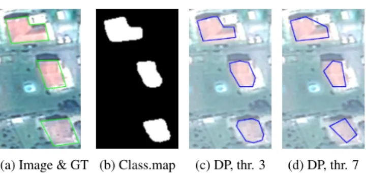
The polygonization challenge is illustrated in Fig. 1, where a classification map obtained by the recent convolu-tional neural network (CNN)-based approach [4] is poly-gonized using Douglas-Peucker method with two different threshold parameters. We can see that in most cases the re-sulting polygons do not represent well the underlying objects. In this work, we aim at building a deep learning-based model, which would be capable to directly output a vectorial
The authors would like to thank ANR for funding the study.
(a) Image & GT (b) Class.map (c) DP, thr. 3 (d) DP, thr. 7
Fig. 1: Example of a polygonization of the classification map. (a) shows a satellite image and vector format ground truth. (b) is a classification map obtained by [4]. (c) and (d) are two polygonization results obtained by Douglas-Peucker method with different thresholds.
semantic labeling of the image. This objective is inspired by a few recent works on using neural networks to output geo-metric objects, such as the convex hull of a point cloud [5] or the coordinates of object bounding boxes [6]. We formulate a mapping problem as a polygon prediction task. The proposed PolyCNNconvolutional neural network takes as input image patches and regresses coordinates of vertices of polygons out-lining objects of interest. The network is built so that it can be trained in an end-to-end fashion. We restricted this study to learning quadrilaterals or 4-sided polygons, the main ob-jective of the study being to demonstrate that we can produce classification maps directly in a vector format and to break a paradigm of two-stage mapping approaches, where raster classification is followed by polygonization.
In the next section, we present the proposed CNN archi-tecture. We then perform experimental evaluation on the So-lar photovoltaic array location and extend dataset (referred to as PV dataset in the following) [7], and draw conclusions.
2. METHODOLOGY
Our PolyCNN network takes as input a color (RGB) image patch centered on the object of interest, and directly outputs the coordinates of a 4-sided polygon in 2D. These image patches can be obtained by using any object detection sys-tem, for instance a Faster-RCNN network [8]. In this work,
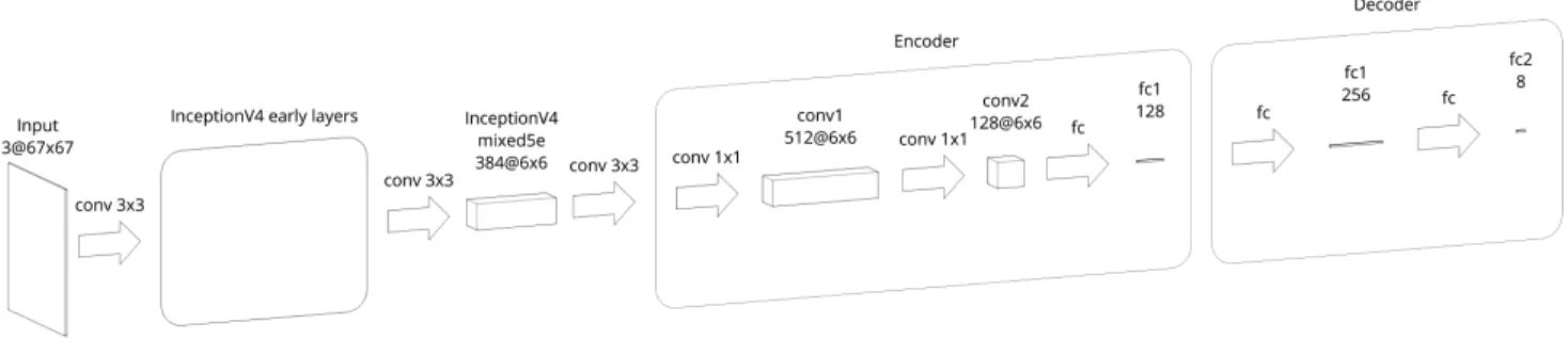
Fig. 2: Architecture of the complete PolyCNN model. The network takes a color image patch as input and directly outputs the coordinates of a 4-polygon in 2D. Activation functions are all ReLUs, except the last activation which is a sigmoid (so that the output coordinates are in [0, 1]). conv = convolutional, fc = fully connected.
we restricted the space of all possible polygons to 4-sided polygons, so that the network has a fixed-length output. An extension to n-sided polygons is a subject of our ongoing work.
2.1. The network
Fig. 2 illustrates the architecture of the proposed PolyCNN model. The neural network is made out of three parts: feature extractor, encoder and decoder. The feature extractor uses the first few layers of a pre-trained Inception V4 network [9] to extract 384 features of resolution 6 × 6. The encoder then computes a vector of dimension 128, that can be seen as a point in a latent space where representing different polygon shapes is easier. The decoder then decodes this 128 vector into the polygonal representation that we are used to: 8 scalars representing the 2D coordinates of 4 points.
To choose the architecture of the encoder and decoder, we experimented on a much simpler dataset. For this purpose, we generated 64 × 64 pixel images of a random white 4-sided polygon on a black background. This simple dataset does not require a complex feature extractor, so we used a very small feature extractor made out of three 5 × 5 convolutional layers (with 8, 16 and 32 channels, respectively), each followed by a 2 × 2 pooling layer. This allowed for fast experimentation, and we found the architecture for the encoder and especially the decoder with the goal of having the smallest model that could learn to regress vertices of 4-sided polygons.
We then had to choose how much of the pre-trained In-ception V4 we needed to use. The InIn-ception V4 was trained on ImageNet [10], whose images are all taken from ground-level. Our model is meant to be trained on aerial or satellite images, which have a very different appearance. Thus only the low-level features of the Inception V4 should be interest-ing, as they are not specific to an object or a point of view and remain general enough. Furthermore, using as few layers as possible has the advantage of yielding a smaller model, which is thus faster to train and is less prone to over-fitting. Using
the first layers of the Inception V4 up to the mixed5e layer seemed to be a good choice regarding the previous consider-ations.
2.2. The loss function
The loss function used to train the PolyCNN network is the mean L2 distance between the vertices of the ground-truth
polygon and the predicted polygon. We note n the number of vertices (here fixed to 4), Pgtthe n×2 matrix representing the groundtruth polygon and Ppredthe n × 2 matrix representing the predicted polygon. See Eq. 1 for the definition of such loss: L = 1 n n X i=1
kPgt(i, .) − Ppred(i, .)k2 (1)
Eq. 1 assumes that both ground-truth and predicted poly-gons have their vertices numbered in the same way (same starting vertex and same orientation). Therefore, this loss function would force the model to learn a specific starting ver-tex. The network cannot learn this, because the starting vertex is arbitrary. A more complex loss has to be used, one which is invariant to the starting vertex. For this purpose, we compute all the possible shifts of vertices for the predicted polygon and take the minimum mean L2distance (to the groundtruth polygon) out of all these shifted polygons. Our loss function is thus defined as:
L = min ∀s∈[0,n−1] 1 n n X i=1 kPgt(i, .) − Ppred(i + s, .)k2 (2)
Eq. 2 still assumes the orientation of both polygons are the same (e.g., clockwise), but we found this not to be a prob-lem: as long as all ground truth polygons have the same ori-entation, the network learns to output polygons with the same orientation.
3. EXPERIMENTAL RESULTS
We use the PV dataset [7] to train, validate and test the per-formance of the proposed network. This dataset contains the
geospatial coordinates and border vertices for over 19000 solar panels (used as ground truth in this work) across 601 high-resolution (30 cm/pixel) aerial orthorectified images from four cities in California, USA.
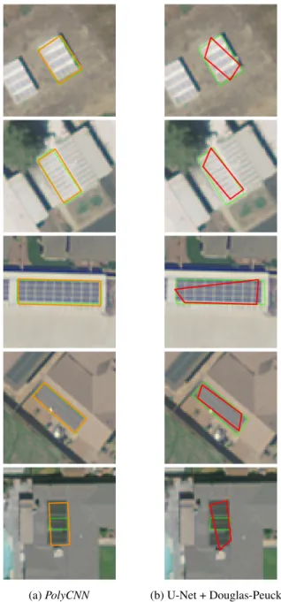
(a) PolyCNN (b) U-Net + Douglas-Peucker
Fig. 3: Examples of visual results on the test set. Ground truth, PolyCNN and baseline polygons are denoted in green, orange and red, respectively.
3.1. Data pre-processing and augmentation
For each image in the PV dataset, we extract square patches of size 67 ·√2 ≈ 95 pixels (the final image patch will be of size 67 pixels, but we need this margin for the data-augmentation step) around each polygon from the ground truth that satisfy the following conditions:
• Number of polygon vertices is 4. All polygons were simplified first because some of them are overdefined (e.g., three aligned vertices).
• Polygon diameter is less than 67 · 0.8 = 53.6 pixels so that enough context is left in the resulting 67 × 67 image patch.
At this point, we have 6366 groundtruth 4-sided polygons each associated to one image patch. Every patch includes at least one polygon and if two polygons are adjacent, two dif-ferent patches are generated, each with its own polygon. We split this dataset into train, validation and test sets. We set both validation and testing set sizes to 256 patches each. This leaves 5854 patches for training. This is a fairly small dataset for training a deep neural network. We performed data aug-mentation to try alleviating this problem, consisting of:
1. Random rotations with angle θ ∈ [0, 2π). 2. Random vertical flip on the rotated image.
Finally, the data is normalized. The image values are scaled between [−1, 1] and the polygon vertex coordinates are scaled between [0, 1].
3.2. Training
The Inception V4 layers are pre-trained on ImageNet [10] and are fine-tuned during training. The Decoder is also pre-trained, this time on the generated dataset of 4-sided polygons we mentioned in the methodology section. We used an Adam optimizer with the default values for the decay rates for the moment estimates β1 = 0.9 and β2 = 0.999. A batch size
of 256 was used. The learning rate (lr) follows a different schedule for the 3 parts of the model:
lr up to iteration 500 1000 90000
Inception V4 layers 0 0 1e − 5
Encoder 1e − 5 1e − 5 1e − 5
Decoder 0 1e − 5 1e − 5
3.3. Results and discussion
To compare our results, we introduce a baseline method to predict 4-sided polygons. It consists of applying U-Net [11] for pixelwise classification (which yielded the highest performance in large-scale aerial image classification chal-lenge [12]) followed by a Douglas-Peucker vectorization algorithm to obtain 4-sided polygons. Because the U-Net can predict several solar arrays within the image patch, it can result in multiple blobs in the prediction image. We thus vec-torize the blob which gives the maximum intersection with the ground truth blob. This way we always obtain a 4-sided polygon around the center of the image, just like our method. Fig. 3 illustrates examples of visual results on the test set. We can observe through the whole test set that our method
Fig. 4: Test set polygon accuracy as a function of the thresh-old in pixels.
outputs polygons which feature better preservation of geomet-ric regularities, such as orientation and close-to-right angles, when compared to the baseline approach.
We use two quantitative measures:
1) Intersection over union (IoU) between the predicted and the ground truth polygons. The proposed PolyCNN and the baseline methods yield a mean IoU of 79.5% and 62.4%, respectively.
2) We introduce a more interesting measure for polygon comparison, which captures well the shape deformation of the prediction polygon. The L2distance between each pair of
vertices is computed (the pair is composed of one groundtruth vertex and its corresponding predicted vertex, the correspon-dence is chosen exactly the same as for the modified loss in Eq. 2). We then compute the fraction of vertices in the whole test set which are closer to their ground truth position than a certain threshold value in pixels, and call it a polygon accu-racymeasure. Fig. 4 shows the obtained polygon accuracy as a function of the threshold in pixels for both approaches.
From the experimental comparison, we can conclude that the proposed PolyCNN network succeeds in learning to pre-dict vertices of 4-sided polygons corresponding to the objects of interest.
Finally, we would like to note that if we train from scratch, i.e. without using the pre-trained Inception V4, the network does not succeed to learn a vectorial semantic labeling. The Tensorflow code of the PolyCNN network will be made avail-able by the time of publication.
4. CONCLUDING REMARKS
We showed that learning directly in vectorial space is pos-sible in a end-to-end fashion and yields better results than a 2-step process involving a U-Net followed by vectorization. Indeed our method can better predict the geometric shape of the object.
The proposed architecture is relatively big with more than 2.7 × 10e6 weights. We will try using a fully-convolutional architecture in the future which should greatly reduce the
amount of weights. Other areas of future experimentation in-clude using different feature extractors (U-Net, SegNet [13]), learning n-sided polygons with variable n and learning to outline other type of objects such as buildings.
5. REFERENCES
[1] M. Visvalingam and J. D. Whyatt, “Line generalisation by repeated elimination of the smallest area,” The Car-tographic Journal, vol. 30, no. 1, pp. 46–51, 1992. [2] D. H. Douglas and T. K. Peucker, “Algorithms for the
reduction of the number of points required to represent a digitized line or its caricature,” The Canadian Cartog-rapher, vol. 10, no. 2, pp. 112–122, 1973.
[3] E. Maggiori, Y. Tarabalka, G. Charpiat, and P. Alliez, “Polygonization of remote sensing classification maps by mesh approximation,” in IEEE ICIP, 2017.
[4] E. Maggiori, Y. Tarabalka, G. Charpiat, and P. Alliez, “High-resolution aerial image labeling with convolu-tional neural networks,” IEEE TGRS, vol. 55, no. 12, 2017.
[5] O. Vinyals, M. Fortunato, and N. Jaitly, “Pointer net-works,” 2015, pp. 2692–2700.
[6] D. Erhan, C. Szegedy, A. Toshev, and D. Anguelov, “Scalable object detection using deep neural networks,” 2014, pp. 2147–2154.
[7] K. Bradbury et al., “Distributed solar photovoltaic ar-ray location and extent dataset for remote sensing object identification,” Scientific Data, vol. 3:160106, 2016. [8] S. Ren, K. He, R. B. Girshick, and J. Sun, “Faster
R-CNN: towards real-time object detection with region proposal networks,” CoRR, vol. abs/1506.01497, 2015. [9] C. Szegedy, S. Ioffe, and V. Vanhoucke, “Inception-v4,
inception-resnet and the impact of residual connections on learning,” CoRR, vol. abs/1602.07261, 2016. [10] J. Deng, W. Dong, R. Socher, L.-J. Li, K. Li, and L.
Fei-Fei, “ImageNet: A Large-Scale Hierarchical Image Database,” in CVPR, 2009.
[11] O. Ronneberger, P.Fischer, and T. Brox, “U-net: Convo-lutional networks for biomedical image segmentation,” in MICCAI, 2015, vol. 9351, pp. 234–241.
[12] B. Huang et al., “Large-scale semantic classification: outcome of the first year of inria aerial image labeling benchmark,” in IGARSS, 2018.
[13] V. Badrinarayanan, A. Kendall, and R. Cipolla, “Seg-net: A deep convolutional encoder-decoder architecture for image segmentation,” CoRR, vol. abs/1511.00561, 2015.