HAL Id: hal-00296299
https://hal.archives-ouvertes.fr/hal-00296299
Submitted on 26 Jul 2007
HAL is a multi-disciplinary open access
archive for the deposit and dissemination of
sci-entific research documents, whether they are
pub-lished or not. The documents may come from
teaching and research institutions in France or
abroad, or from public or private research centers.
L’archive ouverte pluridisciplinaire HAL, est
destinée au dépôt et à la diffusion de documents
scientifiques de niveau recherche, publiés ou non,
émanant des établissements d’enseignement et de
recherche français ou étrangers, des laboratoires
publics ou privés.
major population centers
M. G. Lawrence, T. M. Butler, J. Steinkamp, B. R. Gurjar, J. Lelieveld
To cite this version:
M. G. Lawrence, T. M. Butler, J. Steinkamp, B. R. Gurjar, J. Lelieveld. Regional pollution potentials
of megacities and other major population centers. Atmospheric Chemistry and Physics, European
Geosciences Union, 2007, 7 (14), pp.3969-3987. �hal-00296299�
www.atmos-chem-phys.net/7/3969/2007/ © Author(s) 2007. This work is licensed under a Creative Commons License.
Chemistry
and Physics
Regional pollution potentials of megacities and other major
population centers
M. G. Lawrence1, T. M. Butler1, J. Steinkamp1, B. R. Gurjar2, and J. Lelieveld1
1Max-Planck-Institut f¨ur Chemie, P.O. Box 3060, 55020 Mainz, Germany
2Indian Institute of Technology Roorkee, Department of Civil Engineering, Roorkee 247667, India
Received: 1 December 2006 – Published in Atmos. Chem. Phys. Discuss.: 19 December 2006 Revised: 13 June 2007 – Accepted: 23 July 2007 – Published: 26 July 2007
Abstract. Megacities and other major population centers represent large, concentrated sources of anthropogenic pollu-tants to the atmosphere, with consequences for both local air quality and for regional and global atmospheric chemistry. The tradeoffs between the regional buildup of pollutants near their sources versus long-range export depend on meteoro-logical characteristics which vary as a function of geograph-ical location and season. Both horizontal and vertgeograph-ical trans-port contribute to pollutant extrans-port, and the overall degree of export is strongly governed by the lifetimes of pollutants. We provide a first quantification of these tradeoffs and the main factors influencing them in terms of “regional pollution potentials”, metrics based on simulations of representative tracers using the 3-D global model MATCH (Model of At-mospheric Transport and Chemistry). The tracers have three different lifetimes (1, 10, and 100 days) and are emitted from 36 continental large point sources. Several key features of the export characteristics emerge. For instance, long-range near-surface pollutant export is generally strongest in the middle and high latitudes, especially for source locations in Eurasia, for which 17–34% of a tracer with a 10-day lifetime is ex-ported beyond 1000 km and still remains below 1 km altitude. On the other hand, pollutant export to the upper troposphere is greatest in the tropics, due to transport by deep convection, and for six source locations, more than 50% of the total mass of the 10-day lifetime tracer is found above 5 km altitude. Furthermore, not only are there order of magnitude interre-gional differences, such as between low and high latitudes, but also often substantial intraregional differences, which we discuss in light of the regional meteorological characteristics. We also contrast the roles of horizontal dilution and vertical mixing in reducing the pollution buildup in the regions in-cluding and surrounding the sources. For some regions such as Eurasia, dilution due to long-range horizontal transport
Correspondence to: M. G. Lawrence
(lawrence@mpch-mainz.mpg.de)
governs the local and regional pollution buildup; however, on a global basis, differences in vertical mixing are domi-nant in determining the pollution buildup both around and further downwind of the source locations.
1 Introduction
For the past few thousand years, human populations have been clustering in increasingly large settlements. At present, there are about 20 cities worldwide with a population of ten million or greater (see Table 1), and 30 with a population of about 7 million or greater. These numbers are expected to grow considerably in the near future. This confluence of human activity in so-called “megacities” (e.g. Molina and Molina, 2004) leads to serious issues in municipal manage-ment, such as the coordination of public and private trans-port, solid and liquid waste disposal, and local air pollu-tion. The latter is known to have significant local and re-gional consequences for human health and crop production (e.g. Chameides et al., 1994; Emberson et al., 2001). On the other hand, emissions of longer-lived pollutants from these concentrated population centers can affect atmospheric chemistry on the continental and global scale. The balance between local and long-range effects can be anticipated to depend strongly on regional meteorological and geograph-ical differences. Here we address the question: What are the common features and differences in the regional and long-range dispersion characteristics for air pollutants emit-ted from large, concentraemit-ted urban sources?
We examine this issue using representative, artificial trac-ers in a global 3-D chemistry-transport model (CTM). Three tracers with exponential decay lifetimes of 1, 10, or 100 days are emitted from each of 36 selected major population cen-ters. These can be applied generically towards understand-ing the anticipated typical outflow characteristics of a wide range of trace gases and aerosols. For instance, the typical
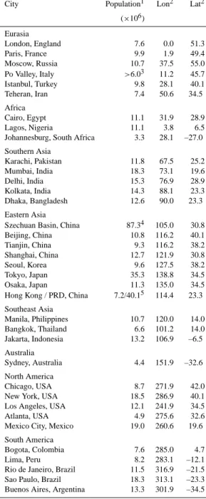
Table 1. The set of selected MPC source locations and their approximate populations (projections for 2005), along with the corresponding
longitudes and latitudes as employed in the model setup.
City Population1 Lon2 Lat2
(×106) Eurasia London, England 7.6 0.0 51.3 Paris, France 9.9 1.9 49.4 Moscow, Russia 10.7 37.5 55.0 Po Valley, Italy >6.03 11.2 45.7 Istanbul, Turkey 9.8 28.1 40.1 Teheran, Iran 7.4 50.6 34.5 Africa Cairo, Egypt 11.1 31.9 28.9 Lagos, Nigeria 11.1 3.8 6.5
Johannesburg, South Africa 3.3 28.1 –27.0 Southern Asia Karachi, Pakistan 11.8 67.5 25.2 Mumbai, India 18.3 73.1 19.6 Delhi, India 15.3 76.9 28.9 Kolkata, India 14.3 88.1 23.3 Dhaka, Bangladesh 12.6 90.0 23.3 Eastern Asia
Szechuan Basin, China 87.34 105.0 30.8
Beijing, China 10.8 116.2 40.1 Tianjin, China 9.3 116.2 38.2 Shanghai, China 12.7 121.9 30.8 Seoul, Korea 9.6 127.5 38.2 Tokyo, Japan 35.3 138.8 34.5 Osaka, Japan 11.3 135.0 34.5
Hong Kong / PRD, China 7.2/40.15 114.4 23.3
Southeast Asia Manila, Philippines 10.7 120.0 14.0 Bangkok, Thailand 6.6 101.2 14.0 Jakarta, Indonesia 13.2 106.9 –6.5 Australia Sydney, Australia 4.4 151.9 –32.6 North America Chicago, USA 8.7 271.9 42.0
New York, USA 18.5 286.9 40.1
Los Angeles, USA 12.1 241.9 34.5
Atlanta, USA 4.9 275.6 32.6
Mexico City, Mexico 19.0 260.6 19.6 South America
Bogota, Colombia 7.6 285.0 4.7
Lima, Peru 8.2 283.1 –12.1
Rio de Janeiro, Brazil 11.5 316.9 –21.5 Sao Paulo, Brazil 18.3 313.1 –23.3 Buenos Aires, Argentina 13.3 301.9 –34.5
1Source (unless otherwise noted): Population Division of the Department of Economic and Social Affairs of the United Nations Secretariat
(2004) and World Urbanization Prospects: The 2003 Revision, Web: http://www.unpopulation.org; compilation accessible at http://www. infoplease.com/ipa/A0884418.html.
2The latitudes and longitudes correspond to the model grid cells in which the tracers are emitted, and do not necessarily correspond exactly
to the locations of the represented cities or regions themselves.
3Exact population figure not found; lower limit estimate based on the sum of the populations of Milano and Turino.
4For a provincial area of 485 000 km, covering about 12 T63 grid cells; from http://en.wikipedia.org/wiki/Sichuan, version from 14:13, 10
July 2007, based on the original source China Statistical Yearbook, 2005, ISBN 7503747382.
5Approximate population of the Pearl River Delta zone; from http://en.wikipedia.org/wiki/Pearl River Delta, version from 07:38, 3 July
lifetime of aerosols (sulfate, organic and elemental carbon, nitrate, etc.) generally lies between 1 and 10 days, and the global mean lifetimes of several key reactive trace gases fall in this range, including O3(∼25 d), CO(∼60 d), NOx(∼2 d),
ethane (∼100 d), propane (∼30 d) and butane (∼3 d). The results of this study are complementary to those in Butler et al. (2007a)1, in which we examine the effect of megac-ity emissions more specifically on global and regional O3
chemistry, based on the megacity emissions work of Gur-jar et al. (2004), GurGur-jar and Lelieveld (2005), and Butler et al. (2007b)2. The generic tracer approach used here allows these results to also be applicable to other classes of airborne pollutants, such as Hg, Pb, and persistent organic pollutants (POPs).
The mean geographical distributions of these tracers are compared making use of a set of metrics which helps quan-tify either the degree of export or the coherent retention of the tracers in the source region. Both horizontal and vertical transport contribute to tracer outflow. Horizontal dispersion in the boundary layer (BL) transports pollutants to other re-gions, where they can still have direct effects on health, agri-culture and visibility. Vertical dispersion, especially by cu-mulus convection, removes pollutants from the surface layer, and in turn transports them to the free and upper troposphere, where the lifetimes of many trace gases and aerosols are much longer, their climate effects (e.g., influence on cirrus properties and as greenhouse gases) are more significant, and the potential exists for further transport into the stratosphere. It is not clear a priori what the relative quantitative roles of horizontal and vertical transport are, and how this might vary on a regional basis; this is examined here in light of the re-gional pollution potential metrics.
Several previous studies have also employed global mod-els to examine the outflow, distribution and influence of pol-lutants on regional, continental and global scales (e.g. Wild and Akimoto, 2001; Stohl et al., 2002; Lawrence et al., 2003a; Kunhikrishnan and Lawrence, 2004; Pfister et al., 2004); a good review of these is provided by Akimoto (2003). In contrast to these studies, which have focused on emissions from various country-scale to continental-scale re-gions (e.g., Europe), here we focus on individual megaci-ties and other major population centers, represented as large point sources for the tracers. An alternative approach to studying the outflow characteristics from these concentrated sources would be to employ a regional model. Such models allow a more detailed analysis of local meteorology and re-gional pollutant distribution, and have provided valuable
in-1Butler, T. M., Lawrence, M. G., Gurjar, B. R., and Lelieveld,
J.: The effects of emissions from megacities on global ozone chem-istry, Atmos. Chem. Phys. Discuss., in preparation, 2007a.
2Butler, T. M., Lawrence, M. G., Gurjar, B. R., van Aardenne,
J., Schultz, M., and Lelieveld, J.: The representation of emissions from megacities in global emissions inventories, Atmos. Environ., in review, 2007b.
sights through detailed studies of individual cities (e.g. Gut-tikunda et al., 2005; de Foy et al., 2006). However, the re-gional model would then need to be set up to simulate sev-eral regions around the world in order to address the ques-tion posed above and to allow a comparative analysis of the outflow characteristics of the full large set of chosen source locations. We hope this study might be followed up by sim-ilar analyses with regional models, and suggest a few points where this may be particularly valuable.
In the following section we provide descriptions of the global model used for the simulations (MATCH), the source locations and tracers, and the metrics considered in this study. Following that, we discuss the qualitative and quan-titative dispersion characteristics for the set of tracers, fo-cusing on three particular issues: low-level long-range ex-port, vertical transport to the upper troposphere (UT), and regional exceedances of density thresholds. Our key conclu-sions are summarized in the final section, along with recom-mendations for future studies. Beyond the discussion pre-sented here, for interested readers we also provide an elec-tronic supplement with a full set of figures for the individual source locations, on an annual and seasonal mean basis, as well as key tables and figures for the tracers with different lifetimes.
2 Methods
2.1 Model description
For this analysis we use the global 3-D Model of Atmo-spheric Transport and Chemistry (MATCH). MATCH is a semi-offline model which has been described and evaluated in detail in Rasch et al. (1997); Mahowald et al. (1997b,a); Lawrence et al. (1999, 2003a); von Kuhlmann et al. (2003); Lang and Lawrence (2005a,b). The model transport and physics parameterizations are mostly based on the CCM3 (Kiehl et al., 1996). MATCH has been used to study a variety of topics, including long range transport of pollution plumes (Lawrence et al., 2003a), and transport by deep convection and its effects on global tropospheric O3 (Lawrence et al.,
2003b; Lawrence and Rasch, 2005). Here we are particularly interested in the quality of the simulated tracer transport, es-pecially in pollutant outflow regions. Previous studies have shown this to be generally very good for CO, C3H8and other
pollution tracers, with correlation coefficients between sim-ulated and observed values often being in the 0.7–0.9 range, and with the main exception being in regions where the emis-sions are not well represented, for example, due to the use of climatological biomass burning emissions (Lawrence et al., 2003a; Gros et al., 2003, 2004; Salisbury et al., 2003).
The simulations discussed here are driven by meteorolog-ical data from the NCEP/NCAR reanalysis project (Kalnay et al., 1996) at a horizontal resolution of T63 (96×192 grid points, or about 1.9◦). There are 28 vertical sigma levels
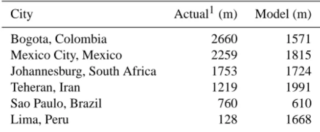
Table 2. The elevations above sea level along with the geopotential
altitudes from the model simulation for the high-altitude MPCs. City Actual1(m) Model (m) Bogota, Colombia 2660 1571 Mexico City, Mexico 2259 1815 Johannesburg, South Africa 1753 1724 Teheran, Iran 1219 1991 Sao Paulo, Brazil 760 610 Lima, Peru 128 1668
1Sources: http://www.hargravesfluidics.com/alt city.php and http:
//en.wikipedia.org
from the surface to about 2 hPa; for a reference surface pres-sure of 1000 hPa, the midpoint prespres-sures of the levels below 100 hPa are: 995.0, 982.1, 964.4, 942.5, 915.9, 883.8, 845.8, 801.4, 750.8, 694.3, 632.9, 568.1, 501.7, 435.7, 372, 312.5, 258.2, 210.1, 168.2, 132.6, and 102.8 hPa. The surface layer is normally 80–90 m thick. The setup is similar to that used in Lawrence et al. (1999) and von Kuhlmann et al. (2003), but focusing only on artificial tracers, and including the new plume ensemble tracer transport representation for deep con-vection from Lawrence and Rasch (2005). The model is run in a “semi-offline” mode, relying only on a limited set of input data fields, which are: surface pressure, geopotential, temperature, horizontal winds, surface latent and sensible heat fluxes, and zonal and meridional wind stresses. These are interpolated in time to the model time step of 30 min, and used to diagnose online the transport by advection, vertical diffusion, and deep convection, as well as the tropospheric hydrological cycle (water vapor transport, cloud condensate formation and precipitation). All runs analyzed here are for the year 1995, which was chosen as a “neutral” year with regards to the ENSO. For the 1 and 10-day lifetime tracers, one month (December, 1994) is used as a spinup, while for the 100-day lifetime tracers a 1-year spinup (1994) is used. 2.2 Tracer emissions and decay
A set of tracers is emitted at the same rate, 1 kg/s, into the model surface layer at each major population center source location. The emission is per grid cell, so that the same mass of each tracer is emitted over time, regardless of the source grid cell location or size (for the larger major population cen-ters, like the Szechuan Basin, the emission is only into the single grid cell with the coordinates given in Table 1). Fol-lowing emission, the tracers are transported with the model parameterizations, and a uniform global decay rate is applied to the tracer mixing ratios each time step. Three characteris-tic decay rates have been chosen: 1 d, 10 d, and 100 d, which correspond to the main range of tracers of interest in urban and regional air pollution, as discussed in the introduction. Wet and dry deposition processes are not included for the
tracers. The tracer mixing ratios are archived on a monthly mean basis.
2.3 Tracer source locations
Table 1 lists the major population centers (“MPCs”) cho-sen for the simulations, along with their approximate pop-ulations and the corresponding closest model grid cell lati-tudes and longilati-tudes at the chosen resolution. Thirty of these MPCs correspond to the worldwide most populated cities in 2000, with populations ranging from about 7 million (Hong Kong, Teheran and Chicago) to more than 20 million (Mex-ico City and Tokyo). Six additional major population centers have also been included, helping to improve the global cover-age: Po Valley, Italy; Johannesburg, South Africa; Szechuan Basin, China; Sydney, Australia; Atlanta, USA; and Bogota, Colombia. Some of the megacities chosen are to an extent representative of even greater metropolitan areas, such as the Pearl River Delta (PRD) adjacent to Hong Kong, and the Boston-New York-Washington (BosNYWash) extended metropolis surrounding New York City. Note that we ac-tually included about ten other source locations in our sim-ulations to further improve the geographical representation, but determined that they did not provide any substantial ad-ditional information beyond the conclusions that are drawn based on the selected set; in a few cases, however, some of these additional tracer results will be referred to below to em-phasize certain points.
The geographical distribution of the locations of the cho-sen MPCs can be seen in Fig. 1, which is discussed in more detail in Sect. 3. Considering first the “proper” megacities, most are in the Northern Hemisphere, and the greatest con-centration of megacities is clearly in Asia, though there is a relatively good global coverage. The coverage is improved considerably with the inclusion of the additional MPCs men-tioned above, especially Johannesburg and Sydney. The ma-jority of the MPCs are either directly coastal, or within about 100 km of a coast (mostly oceanic, though in some cases like the Po Valley, Teheran and Chicago, also near large seas and lakes). Because of this, many of the MPCs are either nearly at sea level or are within a few hundred meters alti-tude. However, there are several exceptions to this, with a few being at very high elevations, as listed in Table 2. In general, the model at the resolution employed (T63) is able to capture the characteristic high elevation of these cities, especially for plateaus like the highveld around Johannes-burg, although it often tends to underestimate the altitude due to the smearing out of detailed orographic features in the model grid cells. One of the main exceptions to this is Lima, for which the geopotential altitude of the corre-sponding model grid is much higher than the actual altitude of the city. This is due to its close proximity to the An-des mountain range, which is partially included in the grid cell including Lima. A few other MPCs are also affected by this interpolation of orography, especially for mountains near
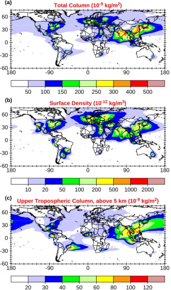
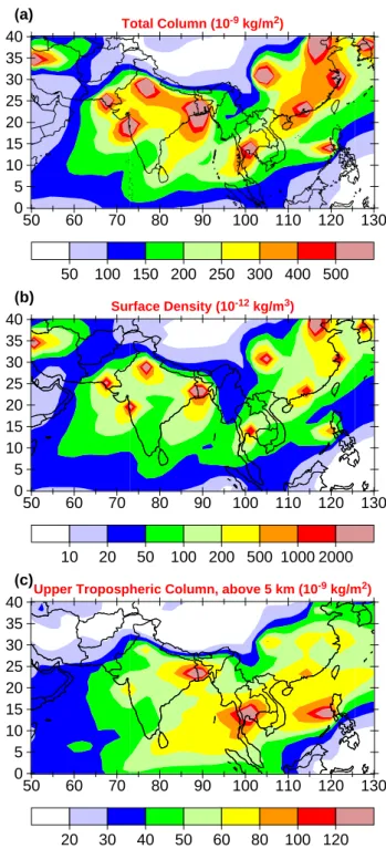
180 -90 0 90 180 -60 -30 0 30 60 180 -90 0 90 180 -60 -30 0 30 60 180 -90 0 90 180 -60 -30 0 30 60 Total Column (10-9 kg/m2) (a) 50 100 150 200 250 300 400 500 Surface Density (10-12 kg/m3) (b) 10 20 50 100 200 500 1000 2000 Upper Tropospheric Column, above 5 km (10-9 kg/m2) (c)
20 30 40 50 60 80 100 120
Fig. 1. The annual mean sum of all τ =10 d MPC tracers for (a)
the total column mass density (10−9kg/m2), (b) the model sur-face layer density (10−12kg/m3), and (c) the column above 5 km (10−9kg/m2).
coasts or valleys, though not as severely as Lima; the main MPCs affected are the Po Valley (modeled altitude: 942 m; actual elevation: ∼100−200 m), the Szechuan Basin (764 m vs. ∼200−500 m), Beijing (740 m vs. ∼40 m), and Rio de Janeiro (600 m vs. ∼10 m; note the proximity to Sao Paulo, listed in Table 2, which is at a much higher altitude than Rio de Janeiro). For these MPCs, it can be expected that the re-sults presented here will be biased towards more long-range transport in the free troposphere and less retention at low al-titudes. The deviations in modeled geopotential altitude for the remaining MPCs, at elevations near sea level, are gener-ally small.
Table 3. Brief descriptions of the metrics used in this study.
Symbol Metric
ELRcol Fraction of total tracer mass which is beyond 1000 km away from the source point (at any al-titude)
ELR1 km Fraction of total tracer mass which is beyond 1000 km away from the source point, and re-mains below 1 km altitude
EUT Fraction of total tracer mass which is above 5 km altitude (at any horizontal location) Ax Total surface area (in 106km2) of the model
grid cells with a tracer density exceeding xng/m3, where x=1, 10, and 100 ng/m3
2.4 Metrics
The metrics which are employed to examine the tracer distri-butions are focused on addressing two main questions:
– How much of the tracer mass is exported beyond a given distance (horizontal and/or vertical)?
– How large is the geographical area surrounding the source location with a substantial pollution buildup? We have examined a wide variety of metrics for quantifying the dispersion of these tracers. In this paper, we focus on a subset of these, summarized in Table 3, which illustrate the main findings regarding global tracer dispersion characteris-tics. The metrics are computed for both monthly and annual mean output, and the ranks of the MPCs are discussed for each metric.
The first basic type of metric is the mass which is ex-ported to a chosen minimum distance away from the city, in the horizontal and/or vertical. For the pollutant export over long ranges (“ELR”) in the horizontal, we focus on the low-level export in terms of the fraction of total tracer mass in the lowest 1 km of the model which is transported to more than 1000 km away from the source location, denoted as ELR1km. We have also considered other distance
thresh-olds (e.g., 500 km, 2000 km), but find the same qualitative results to hold as for 1000 km. This scale, which represents a rough boundary between regional and continental scale pol-lution, should be appropriate for studies with the model at T63 resolution, since a circle with a radius of 1000 km is rep-resented by ∼100 model grid cells. In addition, we briefly note the main results for the overall long-range horizontal export (to beyond 1000 km) at any altitude within the col-umn, ELRcol. Vertical export to the upper troposphere (UT)
is discussed in terms of the fractional mass of each tracer which resides above 5 km, at any horizontal distance from the source (EUT).
To compute ELRcol and ELR1km, it is necessary to
the desired radii surrounding each chosen source point. We approximate such circles by determining the locations of a set of equidistant points around each source point. The trans-formation from distances in meters to the graticule (latitude-longitude grid) is based on the radii of the WGS84 ellipsoid (National Imagery and Mapping Agency, http://earth-info.nga.mil/GandG/publications/tr8350.2/wgs84fin.pdf, 2000). Only the appropriate fraction of the tracer masses are taken for the set of grid cells which are on the boundaries of the circles (i.e., partly inside and outside the circles); for these border grid cells, the assumption is made that they are rectangular, and the fraction inside or outside the circle is calculated as an area weighted factor using the gridcell edges and the spline formed by the equidistant points (the error due to this assumption is <1%, which was tested by summing up the areas enclosed by the circles using this approach versus the actual analytically computed geometric surface area of the circles).
A completely different type of metric which we consider is the geographical area (including the source grid cell), which we denote as Ax, over which the tracer density in the surface layer exceeds a chosen threshold x (in ng/m3). In Sect. 3.3 we consider A1, A10, and A100 (threshold densities 1, 10,
and 100 ng/m3, respectively), mostly focusing on the results for A10. Note that we choose to work in density here, since
this is more commonly applied in air pollution studies (the conversion to mass mixing ratio at the surface is straightfor-ward, since surface air has a density of close to 1 kg/m3). This metric is similar in principle to the “megacity footprint” defined by Guttikunda et al. (2005), in which they consider the area in which the emissions from a megacity contribute to 10% or more of the monthly mean ambient concentrations of real pollutants below 1 km altitude. The metrics A1, A10,
and A100indicate the coherence of the outflow plumes, that
is, the extent to which they remain as concentrated polluted regions (including, surrounding and downwind of the MPC) versus being rapidly dispersed and diluted to lower densities away from the source. We expect this metric to generally be complementary to ELR1 kmand EUT, since they instead
rep-resent the transport and thus dilution of the tracer over large horizontal or vertical distances. The relationship between the metrics in terms of the results from the simulations is dis-cussed in Sect. 3.4.
3 Qualitative and quantitative dispersion characteris-tics
Figure 1 shows the annual mean column-integrated density summed over all of the τ =10 d tracers from the source lo-cations listed in Table 1, along with the surface density and the upper tropospheric column-integrated density. The global outflow figures for the τ =1 d and τ =100 d tracers (see the electronic supplement http://www.atmos-chem-phys.net/ 7/3969/2007/acp-7-3969-2007-supplement.pdf) are
qualita-tively similar to the τ =10 d tracers, though with less (τ =1 d) or more (τ =100 d) effective dispersion, respectively, as could be anticipated from the different lifetimes. In the fol-lowing sections, we discuss the results based on the metrics described in Table 3. In each section, we focus first on the main general results for the τ =10 d tracers, then discuss dif-ferences for the τ =1 d and τ =100 d tracers, along with more specific points for individual MPCs.
3.1 Low-level long-range export 3.1.1 General results
The outflow in the model surface layer (Fig. 1b) can be com-pared to the column densities (Fig. 1a), showing that the re-tention of pollutants near the surface tends to be stronger in the mid- and high-latitudes than in the tropics. For most sources, the surface flow pattern dominates the total (col-umn) outflow; the main exceptions to this are in the tropics, particularly in South America, where much of the mass is lofted to the UT, and the UT flow direction is different than near the surface.
The values of ELR1 km for the τ =10 d tracers are listed
in Table 4. The table gives the annual mean and seasonal variability (standard deviation of the 12 monthly means) for each MPC. Seasonally, the low-level long-range export is al-most uniformly largest during the winter. Overall, the annual mean ELR1 km varies by more than an order of magnitude,
from 34% for Moscow to 3.2% for Jakarta, with an average value of 14.1%, which makes this a good metric for distin-guishing the MPCs in different regions. This is in contrast to the metric ELRcol, which only ranges from 62% to 84%
(not listed in Table 4), implying that it is important to add a vertical component to the long range export, as is done with
ELR1km, in order to distinguish the MPCs well.
The greatest long-range export of pollutant mass near the surface is for the seven source locations in the region of ap-proximately 0◦–50◦E and 25◦–55◦N (Europe, western Asia, and northern Africa), with an average ELR1 km of 23.4%
and an average rank of 5.1. These are followed by the NE Chinese cities (mean ELR1 km=18.4%, mean rank of 9.3),
and by the two northeastern USA source locations (mean
ELR1 km=17.7%, mean rank of 11.5). At the other end, the
lowest values are generally computed for MPCs at high ele-vations (Table 2), for which a reduced ELR1 kmfrom
hori-zontal transport to surrounding, lower-elevation regions can be expected, and for MPCs where there is strong convec-tive activity, removing pollutants from the BL before they can be transported far downwind. Examples include cities in Southeast and East Asian (Manila, Bangkok, Jakarta, and the Szechuan Basin), North and South America (Mexico City, Bogota, Sao Paulo, and Rio de Janeiro), and African (Lagos and Johannesburg), with a mean for these of ELR1 km=5.6%
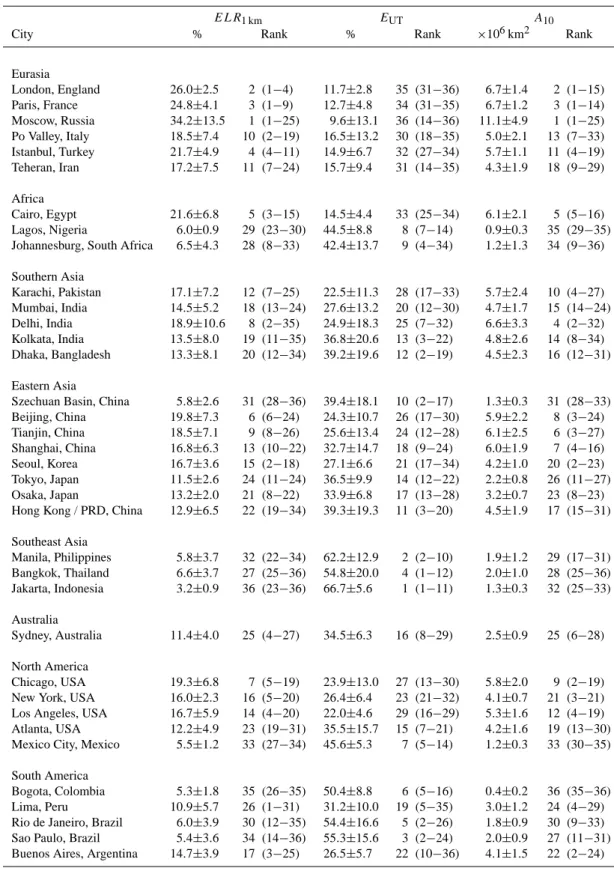
Table 4. Annual mean regional pollution potentials of the selected MPC source locations for the τ =10 d tracers, with ± standard deviations
of the monthly means for the values, and minimum and maximum monthly values (in parenthesis) for the ranks.
ELR1 km EUT A10
City % Rank % Rank ×106km2 Rank
Eurasia London, England 26.0±2.5 2 (1−4) 11.7±2.8 35 (31−36) 6.7±1.4 2 (1−15) Paris, France 24.8±4.1 3 (1−9) 12.7±4.8 34 (31−35) 6.7±1.2 3 (1−14) Moscow, Russia 34.2±13.5 1 (1−25) 9.6±13.1 36 (14−36) 11.1±4.9 1 (1−25) Po Valley, Italy 18.5±7.4 10 (2−19) 16.5±13.2 30 (18−35) 5.0±2.1 13 (7−33) Istanbul, Turkey 21.7±4.9 4 (4−11) 14.9±6.7 32 (27−34) 5.7±1.1 11 (4−19) Teheran, Iran 17.2±7.5 11 (7−24) 15.7±9.4 31 (14−35) 4.3±1.9 18 (9−29) Africa Cairo, Egypt 21.6±6.8 5 (3−15) 14.5±4.4 33 (25−34) 6.1±2.1 5 (5−16) Lagos, Nigeria 6.0±0.9 29 (23−30) 44.5±8.8 8 (7−14) 0.9±0.3 35 (29−35)
Johannesburg, South Africa 6.5±4.3 28 (8−33) 42.4±13.7 9 (4−34) 1.2±1.3 34 (9−36) Southern Asia Karachi, Pakistan 17.1±7.2 12 (7−25) 22.5±11.3 28 (17−33) 5.7±2.4 10 (4−27) Mumbai, India 14.5±5.2 18 (13−24) 27.6±13.2 20 (12−30) 4.7±1.7 15 (14−24) Delhi, India 18.9±10.6 8 (2−35) 24.9±18.3 25 (7−32) 6.6±3.3 4 (2−32) Kolkata, India 13.5±8.0 19 (11−35) 36.8±20.6 13 (3−22) 4.8±2.6 14 (8−34) Dhaka, Bangladesh 13.3±8.1 20 (12−34) 39.2±19.6 12 (2−19) 4.5±2.3 16 (12−31) Eastern Asia
Szechuan Basin, China 5.8±2.6 31 (28−36) 39.4±18.1 10 (2−17) 1.3±0.3 31 (28−33)
Beijing, China 19.8±7.3 6 (6−24) 24.3±10.7 26 (17−30) 5.9±2.2 8 (3−24) Tianjin, China 18.5±7.1 9 (8−26) 25.6±13.4 24 (12−28) 6.1±2.5 6 (3−27) Shanghai, China 16.8±6.3 13 (10−22) 32.7±14.7 18 (9−24) 6.0±1.9 7 (4−16) Seoul, Korea 16.7±3.6 15 (2−18) 27.1±6.6 21 (17−34) 4.2±1.0 20 (2−23) Tokyo, Japan 11.5±2.6 24 (11−24) 36.5±9.9 14 (12−22) 2.2±0.8 26 (11−27) Osaka, Japan 13.2±2.0 21 (8−22) 33.9±6.8 17 (13−28) 3.2±0.7 23 (8−23)
Hong Kong / PRD, China 12.9±6.5 22 (19−34) 39.3±19.3 11 (3−20) 4.5±1.9 17 (15−31) Southeast Asia Manila, Philippines 5.8±3.7 32 (22−34) 62.2±12.9 2 (2−10) 1.9±1.2 29 (17−31) Bangkok, Thailand 6.6±3.7 27 (25−36) 54.8±20.0 4 (1−12) 2.0±1.0 28 (25−36) Jakarta, Indonesia 3.2±0.9 36 (23−36) 66.7±5.6 1 (1−11) 1.3±0.3 32 (25−33) Australia Sydney, Australia 11.4±4.0 25 (4−27) 34.5±6.3 16 (8−29) 2.5±0.9 25 (6−28) North America Chicago, USA 19.3±6.8 7 (5−19) 23.9±13.0 27 (13−30) 5.8±2.0 9 (2−19)
New York, USA 16.0±2.3 16 (5−20) 26.4±6.4 23 (21−32) 4.1±0.7 21 (3−21)
Los Angeles, USA 16.7±5.9 14 (4−20) 22.0±4.6 29 (16−29) 5.3±1.6 12 (4−19)
Atlanta, USA 12.2±4.9 23 (19−31) 35.5±15.7 15 (7−21) 4.2±1.6 19 (13−30)
Mexico City, Mexico 5.5±1.2 33 (27−34) 45.6±5.3 7 (5−14) 1.2±0.3 33 (30−35) South America
Bogota, Colombia 5.3±1.8 35 (26−35) 50.4±8.8 6 (5−16) 0.4±0.2 36 (35−36)
Lima, Peru 10.9±5.7 26 (1−31) 31.2±10.0 19 (5−35) 3.0±1.2 24 (4−29)
Rio de Janeiro, Brazil 6.0±3.9 30 (12−35) 54.4±16.6 5 (2−26) 1.8±0.9 30 (9−33) Sao Paulo, Brazil 5.4±3.6 34 (14−36) 55.3±15.6 3 (2−24) 2.0±0.9 27 (11−31) Buenos Aires, Argentina 14.7±3.9 17 (3−25) 26.5±5.7 22 (10−36) 4.1±1.5 22 (2−24)
180 -90 0 90 180 -60 -30 0 30 60 180 -90 0 90 180 -60 -30 0 30 60 180 -90 0 90 180 -60 -30 0 30 60
Surface Density (10-12 kg/m3) Tau = 1 d (a)
0.5 1 2 5 10 20 50 100
Surface Density (10-12 kg/m3) Tau = 10 d (b)
5 10 20 50 100 200 500 1000
Surface Density (10-12 kg/m3) Tau = 100 d (c)
50 100 200 500 1000 2000 5000 10000
Fig. 2. The annual mean sum of the surface layer densities (10−12kg/m3) of all of the MPC tracers for (a) τ =1 d, (b) τ =10 d, and (c) τ =100 d; note that the data in panel (b) is the same as in Fig. 1b, except with different contour intervals for better compari-son to the other panels.
An important characteristic in terms of the impact of emis-sions on health and agriculture is how much of the long-range export remains over land, and how much is over the oceans. Since most MPCs are near coasts, the mean ELR1 km
lim-ited to only land regions is 6.4%, slightly less than half of the mean ELR1 kmover both surfaces. The values and ranks
of the individual tracers for outflow over land versus outflow over both land and sea are well correlated (the correlation be-tween the rankings is r2=0.88, with a root mean square (rms) deviation of 3.6). Interestingly, this makes the distinction of MPCs at the extreme ends even stronger: for land-export only, the values of ELR1 kmrange from 28.5% for Moscow
(a land-locked city) down to 0.5% for Jakarta (on an island).
How do the results change if we make different choices for the outflow depth, minimum outflow distance, and tracer lifetimes? For the outflow depth, we also examined the val-ues for outflow restricted to only the near-surface layer below 100 m. This results in much smaller exported mass fractions, with ELR100 maveraging 1.5%, close to the factor of 10
dif-ference in the outflow volumes, but the rankings are nearly identical to those listed in Table 4 (r2=0.99, rms=1.0). For the dependence on the outflow distances, we can compare the results for outflow beyond either 500 km or 2000 km, and find again that the rankings compared to outflow beyond 1000 km do not change significantly (r2=0.98, rms=1.5, and
r2=0.91, rms=3.2, respectively).
There are more notable differences for the rankings of the
τ =1 d and τ =100 d tracers compared to the τ =10 d tracers (r2=0.55, rms=7.5, and r2=0.69, rms=6.1, respectively). To give a better indication of the overall similarity and differ-ences in the outflow depending on the tracer lifetime, the surface layer outflow for the tracers with the three different lifetimes are plotted in Fig. 2. Since the total global masses of the tracers are proportional to their lifetimes, the contour intervals are also chosen scaled by the lifetimes (e.g., 10× larger for τ =10 d than for τ =1 d). While the τ =1 d tracers tend to remain relatively concentrated near their source lo-cations, the τ =10 d tracers disperse readily over continental scales, though they still show substantial peaks in the densi-ties over large regions near their sources. Much of the mass of the τ =100 d tracers, on the other hand, is spread out over the Northern Hemisphere, in the lowest contour interval, and the peak densities at the sources are much less pronounced. More specific differences related to tracer lifetime are dis-cussed in the following section.
3.1.2 Specific MPC features
Although there is a general regional classification in the be-havior of the tracers from the MPCs, as discussed above, there are also several notable intra-regional differences in
ELR1 km between MPCs in specific regions. One example
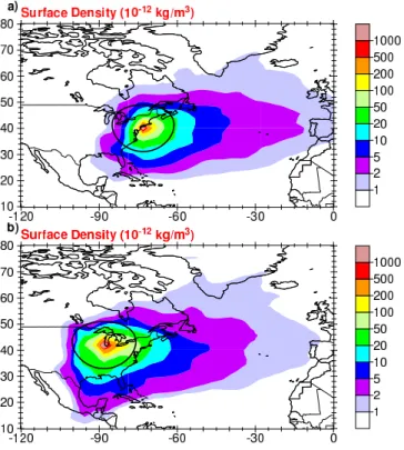
is northeastern North America, where frontal disturbances along the east coast of the USA result in tracers being readily lofted by warm conveyor belts (Stohl, 2001), reducing the re-tention of pollutants near the surface, and thus their potential for long-range low-level export. This results in a less effec-tive export for New York (rank 16) versus nearby Chicago (rank 7), as depicted in Fig. 3 (we also examined additional tracers for Montreal and Toronto, which had ELR1 kmvalues
very similar to Chicago).
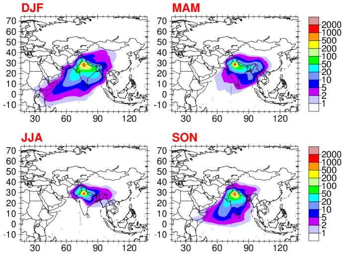
Another notable difference is in southern Asia, where the Asian summer monsoon convection is much stronger towards southern and eastern India and neighboring countries com-pared to its western side (see Fig. 4). This results in the northern and western cities of Delhi (rank 8) and Karachi (rank 12) being considerably more efficient low-level ex-porters than Mumbai (18), Kolkata (19) and Dhaka (20). In
Fig. 3. The annual mean surface layer densities (10−12kg/m3) of the τ =10 d tracers for (a) New York and (b) Chicago; the black circles depict a 1000 km radius around the source locations.
Eurasia plus Cairo, where the values and the ranks are all generally high, there is nevertheless nearly a factor of two spread between Teheran and Moscow, and a very good anti-correlation (r2=0.94) between ELR1 kmand EUT, indicating
the importance of convective lifting in determining the export efficiency. South America and southern North America are similarly influenced by intraregional differences in convec-tive activity, where Buenos Aires (17) and Lima (26) retain greater amounts of pollution in the boundary layer and are thus more efficient exporters than the rest of the South Amer-ican MPCs plus Mexico City (30–35). Likewise, Melbourne, Australia (one of the additional MPCs not selected for Ta-ble 4), in the less convective southern region of Australia, has a value of ELR1 km=20.0%, nearly twice that of Sydney
(ELR1 km=11.4%).
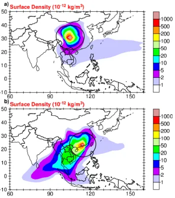
Beyond the differences in vertical lofting due to deep con-vection and warm conveyor belts, gradients in horizontal winds can also lead to large intraregional differences. An example of this is the Szechuan Basin tracer versus the Hong Kong and Pearl River Delta tracers (and to an extent other eastern Asian MPCs). The mean surface layer winds for January, 1995, for this region are depicted in Fig. 5; other months show a similar contrast between the coastal and in-land regions, though less extreme due to the seasonal rever-sal of the mean wind direction in coastal eastern Asia dur-ing the summer monsoon. The contrastdur-ing effects of the
lo-Fig. 4. Annual mean convective mass flux through 500 hPa (g/m2/s) for the southern Asian region.
Fig. 5. January mean surface layer winds for the Asian region; the markings indicate the locations of four selected MPCs: SZ – Szechuan Basin, H – Hong Kong, T – Tianjin, S – Seoul.
cal circulation on the Szechuan and Hong Kong tracers are shown in Fig. 6. In this case, the differences in the tracers are not due to the transport out of the BL into the UT, which is nearly the same for the two tracers, and strong in both cases, with EUT=39.3% for Hong Kong and EUT=39.4%
for the Szechuan Basin tracer. Instead, the tracer mass which is left behind in the BL near the Szechuan Basin tends to re-main near its source due to the low-level convergence and recirculation in this region, while in the BL off the coast of Hong Kong the tracer is transported rapidly away by the strong monsoon winds. This results in a value of ELR1 km
for Hong Kong (12.9%) which is over twice as large as for the Szechuan Basin (5.8%).
There is a pronounced seasonality for several MPCs, espe-cially those in southern and eastern Asia, which are affected by the seasonal reversal of the monsoon winds and associated
Fig. 6. The annual mean surface layer densities (10−12kg/m3) of the τ =10 d tracers for (a) the Szechuan Basin and (b) Hong Kong; the black circles depict a 1000 km radius around the source loca-tions.
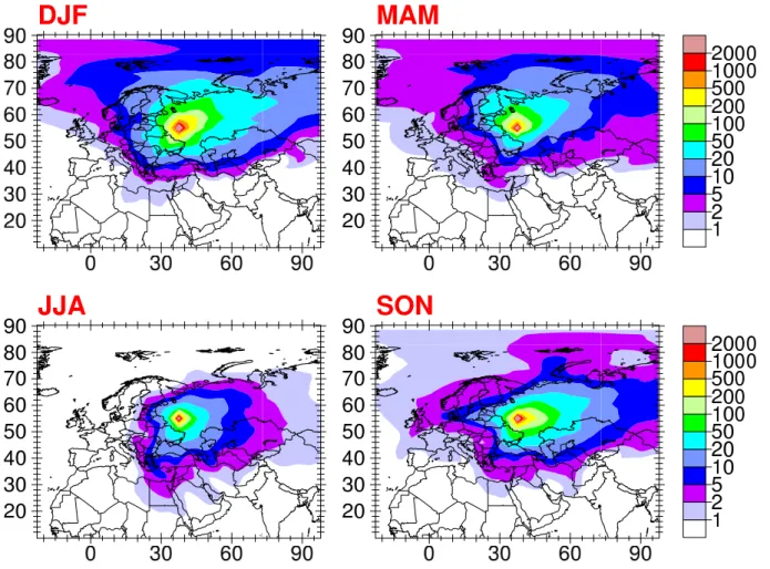
changes in deep convection. An example of this is shown in Fig. 7 for Delhi. In December, Delhi has rank 2 for ELR1 km.
In summer, on the other hand, when the intertropical conver-gence zone (ITCZ) over India causes effective lifting in the monsoon convection, Delhi actually becomes one of the least effective MPCs for low-level pollution export, with a rank of 35. The electronic supplement shows that in most other re-gions the main geographical dispersion patterns (i.e., outflow directions) tend to be more similar for the MPCs throughout the year, though with a few exceptions. One of the most no-table exceptions is Moscow (Fig. 8), which has a strong out-flow into the Arctic during the winter and spring, but primar-ily towards the south during summer. Istanbul, about 15◦S and 10◦W of Moscow, has a similar seasonal variability in the geographic patterns of the outflow, but much less outflow reaching the far northern high latitudes. This contribution of Eurasian cities to the so-called “Arctic haze” is similar to what has been noted in previous studies (e.g. Stohl et al., 2002), which have indicated that generally Eurasian pollu-tion should contribute more strongly to the Arctic haze than North American or eastern Asian emissions. Here we con-firm this to be the case (see the electronic supplement for the full set of comparative figures), and show that the ex-tent of pollution is substantial for a 10-day lifetime tracer, so that this will apply to important real pollutants like O3 and
aerosols. However, we additionally find that the effective-ness per kg of emissions from Moscow in contributing to the Arctic haze is nearly an order of magnitude greater than that of emissions from Paris or London, and furthermore that the seasonal variability of those two western European cities is much less than that of Moscow.
Finally, there are several interesting cases where the re-gional meteorology results in tracers of one lifetime having a notably higher rank (i.e., relatively more effective export beyond 1000 km) than the other two lifetime tracers from the same MPC. Various processes can contribute to this. One such scenario is when regional export tends to occur first in the BL, or in an overlying residual layer above the marine boundary layer, spreading over several thousand km at low altitudes before finally encountering a region of strong mix-ing out of the BL, such as the ITCZ. This results in a rela-tively much more efficient export for the τ =10 d tracers than for either the τ =1 d or τ =100 d, which is found for several cities, including Delhi, Mumbai, Kolkata, Karachi, Beijing, Tianjin, and Cairo. For Delhi, the most extreme case, the annual mean τ =10 d tracer has a rank of 8, while the τ =1 d and τ =100 d tracers have ranks of 25 and 19, respectively. For real tracers this implies that those with intermediate life-times, especially aerosols, will be most important to focus on in terms of controlling downwind pollution from these cities. The secondary convective entrainment downwind can be seen for several MPCs in the electronic supplement, espe-cially well for Kolkata. This type of coherent outflow over the time-scale of about a week has been studied in various field campaigns, in particular for the Asian winter monsoon during the Indian Ocean Experiment (INDOEX) (Lelieveld et al., 2001; Ramanathan et al., 2002), for which MATCH was shown to accurately simulate the sharp transition be-tween polluted Northern Hemisphere and cleaner Southern Hemisphere surface-layer airmasses at the ITCZ (Lawrence et al., 2003a).
The outflow can also encounter regions of strong lofting out of the BL much sooner after leaving the MPC source locations, which results in a relatively more efficient export for the τ =1 d tracers; Manila and Hong Kong are examples where this occurs (Hong Kong has ranks 5, 22 and 29 for
τ =1 d, 10 d, and 100 d, respectively). At the other extreme, for a few MPCs, including the Po Valley, Buenos Aires, Rio de Janeiro, and Johannesburg, the τ =100 d tracer is much more effectively exported relative to the shorter lifetimes tracers. The Po Valley is the most extreme case for this (with ranks 22, 10 and 4 for τ =1 d, 10 d, and 100 d, respectively). In this case, the shorter-lived tracers are effectively retained in the basin region, and along with the stronger convective lofting, this makes the Po Valley less effective for low-level export than the nearby Eurasian MPCs (Moscow, London, Paris and Istanbul). The longer-lived (τ =100 d) tracers, how-ever, can more readily leave the basin region and be exported into the BL of the surrounding regions, making it more sim-ilar to the other Eurasian tracers (Moscow, London, Paris
Fig. 7. Seasonal mean surface layer density (10−12kg/m3) of the τ =10 d tracer for Delhi.
and Istanbul are ranked 1, 2, 3, and 5, respectively, for the
τ =100 d tracers).
3.2 Vertical export to the UT 3.2.1 General results
Transport of certain pollutants from MPCs to the upper tro-posphere (UT) can be important for various global pollu-tion and climate-related issues: for instance, cirrus clouds in the UT contribute significantly to the global long- and short-wave radiation budget, and may be affected by the upwards transport of pollutants which influence the availability of ice nuclei (e.g., Lohmann, 2002); greenhouse gases such as O3
are more effective in the UT due to the colder temperatures (Lacis et al., 1990); the lifetimes of many gases and aerosols tend to be much longer in the UT than near the surface; and the UT serves as the gateway to the stratosphere, for instance for halogenated gases which can affect the stratospheric O3
layer (WMO, 2002). It is important to recall that the tracers considered here are all insoluble tracers; washout of solu-ble tracers will substantially reduce their transport to the UT. A rough rule of thumb (Crutzen and Lawrence, 2000) is that
for soluble tracers with Henry’s Law coefficients of 103, 104, and 105M/atm, the transport to the UT will be about 15%, 50% and 85% as efficient, respectively, as the transport of an insoluble tracer. We plan a more detailed analysis of the fate of soluble tracers in a follow-up study.
Figure 1c shows the column density above 5 km for all the τ =10 d MPC tracers, and Table 4 lists the fractional masses of the MPC tracers which reside above 5 km (EUT).
The variability in EUT between the MPCs is substantial,
mainly reflecting the global variability in convective activ-ity, with values ranging from 9.6% for Moscow to 66.7% for Jakarta. This broad range of values makes EUTa good
met-ric for separating the MPCs. The variability is greater for the
τ =1 d tracer, with EUT ranging from 0.4–45.7%, while for
τ =100 d tracer the range is reduced to 34.0–57.7%. Never-theless, despite the differences in absolute values, the ranks are generally similar (more so than for ELR1 km), with
cor-relations and deviations between the rankings of the τ =1 d and τ =10 d tracers of r2=0.88, rms=3.6, and between the
τ =10 d and τ =100 d tracers of r2=0.72, rms=5.7. It is worth noting that an even greater spread in the values than com-puted here would be expected for any trace gases or aerosols with lifetimes that increase with altitude, since this would
Fig. 8. Seasonal mean surface layer density (10−12kg/m3) of the τ =10 d tracer for Moscow.
result in a greater global mass for the tracers with more ef-ficient export to the UT (whereas using the current setup provides a lower limit to the variability, since all tracers of a given lifetime, e.g., τ =10 d, have the same global total mass).
The strongest export to the UT occurs for the tropical MPCs. A relatively strong anti-correlation is computed be-tween EUTand the absolute latitude of the MPCs (r2=0.63
for τ =10 d). This is mainly due to the greater intensity of deep convection in the tropics, and is reflected in the good correlation (r2=0.63) between EUTand the
parameter-ized convective mass flux through 5 km altitude in the MPC source column for the τ =10 d tracers. For τ =1 d the correla-tion improves to r2=0.81, while for the τ =100 d tracers it is much poorer (r2=0.32), as could be expected due to the less important role of episodic convective mixing for longer-lived tracers.
3.2.2 Specific MPC features
The potential for transporting short and intermediate lifetime insoluble pollutants to the UT is substantial for several of the MPCs. For the τ =10 d tracers, there are 6 source
loca-tions with >50% of the tracer mass in the UT, all in either Southeast Asia or tropical South America: Jakarta, Manila, Bangkok, Sao Paulo, Rio de Janeiro, and Bogota. Even for the τ =1 d tracers, these six MPCs plus one other (Lagos) have >30% of the tracer mass in the UT. At the other end of the spectrum, the lowest seven ranked MPCs for EUTare
all in Eurasia and northern Africa, with an average EUT of
13.7%.
As for ELR1 km, there is a notable intraregional
variabil-ity for several of the MPCs. A clear anti-correlation between
EUTand the absolute latitude of the MPCs was noted above;
the intraregional variability is reflected in several outliers to this anti-correlation. On the high side are MPCs where stronger convection than expected for that latitude prevails throughout much of the year, including Sao Paulo, Rio de Janeiro, Tokyo, Osaka, Manila, and Bangkok. On the low side are cities where convection is suppressed, especially Cairo and Teheran in the downward branch of the Hadley Cell. For Cairo, only half as much makes it to the UT as would be expected from the linear regression on the latitude. One of the clearest intraregional difference is in southern Asia, which is detailed in Fig. 9. This could be anticipated
from the gradient in annual mean convective mass fluxes through 500 hPa (Fig. 4). The stronger mass fluxes to-wards the east and the Bay of Bengal result in a notably stronger upwards transport of pollution from Kolkata and Dhaka (EUT=36.8–39.2%) than from Karachi, Mumbai, and
Delhi (22.5–27.6%), which are in the same latitude range but some 15–20◦ to the west, with the difference growing larger for the cities farther to the west. There are also a few other notable intraregional differences. In South America, the Brazilian MPCs and Bogota are much more efficient ex-porters to the UT (EUT=50.4–55.3%) than Lima and Buenos
Aires (26.5–31.2%), and the difference noted in the previous section between Sydney and Melbourne is seen here as well, with a factor of two difference between the EUT values of
34.5% and 17.2%, respectively.
On the whole, the results from these individual MPCs are reflected in a strong anti-correlation between the full set of EUT and ELR1 km, with r2=0.82 for the values, and
r2=0.89 for the rankings (for the τ =10 d tracers). Thus, vertical transport by convection is a major factor in reduc-ing long-range low-level export. A remainreduc-ing question is how this interplay between vertical and long-range horizontal transport affect the buildup of pollution in the surface layer of the regions surrounding the MPCs, which is addressed in the following sections.
3.3 Regional exceedances of density thresholds 3.3.1 General results
The effects of pollutants on humans and agriculture depends on the amount of the pollutant present (in terms of either the density, concentration or mixing ratio), though the exact de-pendence differs for each pollutant, in terms of both the crit-ical amounts and the exposure time-scales. In this section we examine a regional pollution potential metric which in-dicates the anticipated degree of widespread exposure to ele-vated pollutant levels above a chosen threshold density, in the outflow of each MPC. We focus on the three threshold densi-ties 1, 10, and 100 ng/m3(i.e., A1, A10, and A100), which we
find to be appropriate for characterizing and comparing the outflow of the tracers with all three lifetimes. The physical meaning of these metrics is shown graphically in Figs. 7 and 8 for Delhi and Moscow, and for the remaining MPCs in the electronic supplement, in which A1is represented by the area
enclosed by the light violet shading, A10is the area enclosed
by the light blue shading, and A100is the area enclosed by
the light green shading.
The values for one of these metrics, A10, are given in
Ta-ble 4 for the τ =10 d tracer. The values range over more than an order of magnitude, from 0.4−11.1×10⁶km2, offering a good separation between the MPCs. The MPCs which show the most extensive surface-layer pollution buildup around the source region include those in Europe, western Asia, north-ern Africa, eastnorth-ern China, and eastnorth-ern North America, and
50 60 70 80 90 100 110 120 130 0 5 10 15 20 25 30 35 40 50 60 70 80 90 100 110 120 130 0 5 10 15 20 25 30 35 40 50 60 70 80 90 100 110 120 130 0 5 10 15 20 25 30 35 40 Total Column (10-9 kg/m2) (a) 50 100 150 200 250 300 400 500 Surface Density (10-12 kg/m3) (b) 10 20 50 100 200 500 1000 2000
Upper Tropospheric Column, above 5 km (10-9 kg/m2) (c)
20 30 40 50 60 80 100 120
Fig. 9. Like Fig. 1, except zoomed in on the southern Asian region: (a) the total column mass density (10−9kg/m2), (b) the model sur-face layer density (10−12kg/m3), and (c) the column above 5 km (10−9kg/m2).
the least effective MPCs in the annual mean include those in Southeast Asia, Mexico City, the South American cities of Bogota, Rio de Janeiro and Sao Paulo, the central and southern African cities of Lagos and Johannesburg, and the Szechuan Basin in China.
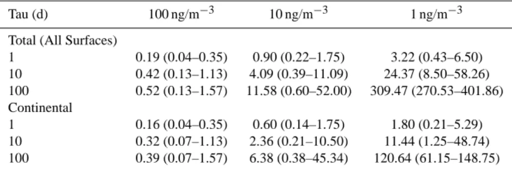
Table 5. Mean surface areas (106km2) with densities exceeding the stated threshold for the given tracer lifetimes (minimum and maximum values are given in parentheses).
Tau (d) 100 ng/m−3 10 ng/m−3 1 ng/m−3 Total (All Surfaces)
1 0.19 (0.04–0.35) 0.90 (0.22–1.75) 3.22 (0.43–6.50) 10 0.42 (0.13–1.13) 4.09 (0.39–11.09) 24.37 (8.50–58.26) 100 0.52 (0.13–1.57) 11.58 (0.60–52.00) 309.47 (270.53–401.86) Continental 1 0.16 (0.04–0.35) 0.60 (0.14–1.75) 1.80 (0.21–5.29) 10 0.32 (0.07–1.13) 2.36 (0.21–10.50) 11.44 (1.25–48.74) 100 0.39 (0.07–1.57) 6.38 (0.38–45.34) 120.64 (61.15–148.75)
A summary of the mean values and ranges of A1, A10, and
A100 for the MPC tracers with the three lifetimes (τ =1 d,
10 d and 100 d) is given in Table 5 for all surface types (land and sea), as well as for the outflow only over continental sur-faces. Since these are linear tracers, these threshold densi-ties will scale with the source magnitude; e.g., for a source of 1000 kg/s, the threshold densities would be 1, 10, and 100 µg/m3. Note, however, that this can only be applied di-rectly for pollutants which do not affect their own loss fre-quencies; for cases where chemical feedbacks are important, such as CO (Prather, 1996) and NOx (Kunhikrishnan and
Lawrence, 2004), a simple scaling like this is not possible. Table 5 shows that, for our case with a source of 1 kg/s for each tracer, the chosen range of threshold densities (1– 100 ng/m3) separates the densities which are generally only found on local to regional scales (<106km2) and the densi-ties which are normally computed to be spread over continen-tal scales (>106km2). The threshold density of 100 ng/m3 is only exceeded over limited regions, with A100 being less
than 106km2 for all tracers (with the one exception being Moscow), and averaging about 0.5×10⁶km2or less, depend-ing on the lifetime (equivalent to a radius of expansion of
≤400 km). On the other hand, the lower threshold density of 1 ng/m3is exceeded over regions much larger than 106km2 for all of the tracers (with the single exception of the τ =1 d tracer for Bogota), averaging up to more than 300×106km2 for the τ =100 d tracers.
The strong concentration of the τ =1 d tracers versus the extensive dispersion of the τ =100 d tracers can be seen quan-titatively by comparing the values in Table 5 with the theo-retical maximum areas which could be covered by the trac-ers for each combination of threshold density and lifetime (assuming instantaneous mixing). For the τ =100 d tracers, the mean value of A1 is fairly close to the maximum
pos-sible value of about 864×106km2(computed assuming the tracers are well-mixed up to 10 km altitude), whereas the ex-tensive dispersion of the long-lived tracers reduces the mean value of A100to less than a tenth of its potential maximum
of 8.64×10⁶km2. The opposite is the case for the τ =1 d tracers. In this case, the strong concentration of these
short-lived tracers around their source locations results in a mean value for A100that is nearly a fourth of the maximum
possi-ble value (0.864×10⁶km2, assuming for this case a mixing depth of 1 km altitude), whereas the limited dispersion re-duces A1 to only about 4% of the maximum possible value
(86.4×10⁶km2).
As for ELR1 km, an additional relevant characteristic is
how much of the regional pollution buildup is over land, and how much is over the oceans. Table 5 shows that for the lower threshold density (1 ng/m3), like for ELR1 kmthe
proximity of most of the MPCs to coasts results in a reduc-tion of the mean value of A1by about one half. For the higher
threshold of 100 ng/m3, however, there is only a small dif-ference between the mean A100for land only and for all
sur-faces, since the regional coverage is generally limited to the area very closely surrounding the MPCs.
Finally, as for the other metrics, we can expect A10 (and
likewise A1 and A100) to vary as a function of the tracer
lifetime and the chosen threshold density. Focusing on the source grid cell, interestingly, the maximum mixing ratios computed for the tracers do not differ much. These are 3.3, 4.8 and 4.5 µg/m3for the τ =1, 10 and 100 d lifetime trac-ers, in all cases much lower than the theoretical maximum of 225−435 µg/m3if all the emissions of a given tracer were to remain concentrated only in the source cell. Since the source rate is the same (1 kg/s) for all three lifetimes, this indicates that the tracer density near the source depends primarily on the dispersion rate, rather than on the lifetime of the tracer within the range considered, τ =1−100 d (that is, the mod-eled dispersion of air away from the source is occurring on time-scales of the order of a day or less). However, it is im-portant to note that transport at the single grid cell scale is difficult to resolve, and it would be valuable to have a confir-mation of this conclusion in a future study using a regional model.
The overall importance of tracer lifetime on larger scales is seen in Fig. 2, which shows the substantial difference in local pollution buildup versus long-range export due to the differ-ent lifetimes. Since the contours have been chosen to reflect the ratios between the total global masses of the tracers, if the
tracers were distributed similarly, despite their different total masses, the figures would look the same. The differences in the panels directly reflect the greater degree of dispersion of the longer-lived tracers. A key question, given these dif-ferences in dispersion, is whether or not the rankings tend to be similar for the various lifetimes. On the whole this is indeed the case, especially for the two longer-lived tracers; for example, for the metric A10 listed in Table 4, the
cor-relations and deviations between the rankings of the τ =1 d and τ =10 d tracers are r2=0.67, rms=6.3, and between the
τ =10 d and τ =100 d tracers are r2=0.83, rms=4.3.
3.3.2 Specific MPC features
There are several notable intraregional differences in A10for
the τ =10 d tracers. As noted above, for the case of Eura-sia this is largely due to differences in deep convective mass fluxes, removing tracers from the BL. Four of the Eurasian MPCs have very high ranks (London – 2, Paris – 3, Moscow – 1, Cairo – 5), while three are ranked much lower (Po Val-ley – 13, Istanbul – 11, Teheran – 18), and there there is a very good anti-correlation between the values of EUT and
A10(r2=0.83, or r2=0.76 if Moscow is not included as an
extreme case).
Another intraregional difference, which was not noted as clearly in the other metrics, is in eastern Asia, where Tianjin, Beijing and Shanghai are ranked 6–8 for A10, while Seoul,
Tokyo, and Osaka are ranked 20–26. In this case, the dif-ference is not due to the vertical transport by convection, rather to differences in the surface wind flow, as depicted in Fig. 5. The contrast is particularly evident for Tianjin and Seoul (“T” and “S” on the figure), which are at about the same model latitude and about 10◦ apart in longitude, and have values of EUTwhich are very close (25.6 and 27.1%).
However, the much lower wind speeds near Tianjin allow considerably more local pollution buildup to a much larger value for A10than for the Seoul tracer (6.1 vs. 4.2×10⁶km2).
3.4 Relationship between long-range low-level export and local to regional pollution buildup
The metrics discussed in the previous three sections can be used in tandem to examine the relative roles of horizon-tal versus vertical transport in determining pollutant export and local to regional pollution buildup around the MPCs. If the vertical mixing were to be the same for two MPCs, then one would expect that more efficient long-range export would tend to dilute the tracer near its source, resulting in smaller regions with elevated tracer densities and thus an anti-correlation between ELR1 kmand Ax(with x=1, 10, or 100). On the other hand, increased vertical mixing out of the BL can lead to a simultaneous reduction in both ELR1 km
and Ax, resulting in a correlation between the two if there are very large differences in vertical mixing between a set of MPCs.
Fig. 10. Scatter plot and least squares regression line between the annual mean values of A100and ELR1 kmfor the τ =10 d trac-ers; the points are coded by their ranks for EUT, with the symbols:
points (·) for the top 10 ranked MPCs, stars (*) for the MPCs ranked 11–17, crosses (×) for ranks 18–29, circles (◦) for ranks 30–35, and a plus (+) for the outlier Moscow (rank 36).
The relationship between ELR1 kmand A100 is shown in
Fig. 10. We focus on the τ =10 d tracers here, for which we expect the relationships to be stronger than for the τ =1 d and
τ =100 d tracers, since convective mixing time-scales in the atmosphere are of the order of 10 days (WMO, 2002); how-ever, the main points discussed here also largely apply to the longer and shorter lived tracers as well. Since we are inter-ested in separating the behavior at local to regional versus continental export scales, we focus on A100, which is limited
to an area equivalent to less than a 1000 km radius circle for all of the tracers (see Table 5). To additionally consider the influence of vertical mixing, the points are coded by different symbols for different values of EUT.
The figure nicely shows the influences of both horizontal and vertical mixing. In particular, for the Eurasian MPCs ex-cluding Moscow (the circles), which have the overall weakest vertical transport (EUT=11.7−16.7%), there is a very strong
anti-correlation between ELR1 kmand A100 (r2=0.80).
In-terestingly, the next set of tracers in terms of values of EUT
(crosses) divide themselves up into two distinct groups, one clustering with the circles (with EUT ranging from 22.0–
32.7%), the other with the stars (EUT=22.5−31.2%). We
have not yet been able to determine a clear reason for this split, but do note that the latter group includes mostly MPCs which are near major coastal export regions (e.g., Seoul, dis-cussed in the previous section), whereas the former group tends to be more inland or have a weaker outflow to mar-itime regions (e.g., Tianjin), and thus the difference between the depth of the continental and marine boundary layers may play a role in this split. Considering these two groups of
MPCs individually, both also show an anti-correlation be-tween ELR1 km and A100 (r2=0.34 and r2=0.81,
respec-tively), again demonstrating the importance of horizontal transport differences between these MPCs.
On the other hand, once the vertical transport becomes more substantial (EUT>33%, stars and points), the
anti-correlation between ELR1 km and A100 breaks down. The
overall importance of the large variability in vertical trans-port between the MPCs can be seen by comparing the clus-ters of the different symbols, which show a decrease in both ELR1 km and A100 with an increasing EUT.
Consid-ering the full set of MPCs, there is a relatively good cor-relation between ELR1 km and A100 (r2=0.60), as well as
an anti-correlation between EUTand ELR1 km(noted above,
r2=0.82) and between EUTand A100(r2=0.45). Thus, from
a global perspective, it is the transport into the free and up-per troposphere, rather than long-range horizontal transport, which is primarily responsible for diluting the surface-layer pollutant levels near their source locations, though for spe-cific regions, or for MPCs in different regions with similar vertical transport characteristics, the trade-off between long-range horizontal export and dilution of pollutants in the re-gion surrounding their sources becomes evident.
4 Conclusions
This study has taken several steps towards developing an overall understanding of the characteristics of pollutant out-flow, long-range pollutant export and regional pollution buildup for emissions from major population centers (MPCs) distributed around the world. The MPCs have been repre-sented as large point sources of tracers with different life-times. Our analysis has focused particularly on bringing out the tradeoffs between local and regional near-surface pollu-tant buildup, low-level long-range export to neighboring re-gions and states, and export to the UT and potentially the lower stratosphere, each as a function of the source location. For this study, we have developed a new approach for ex-amining the comparative characteristics of pollutant disper-sion from MPCs, by defining a set of various metrics tar-geting examination of different outflow and regional pollu-tion buildup characteristics. In principle, the same approach could be applied to future model studies of other source types, such as forest fires (e.g. Heald et al., 2003) and power plants (e.g. Marufu et al., 2004). Since we have employed simple tracers with equal source strengths for all MPCs, the focus has been on the generic meteorological outflow char-acteristics, rather than specific gases and aerosols. A few im-plications of the results for real world tracers were noted in the text, and further implications for ozone and related gases are discussed in Butler et al. (2007b)2.
Using the chosen set of tracers and metrics, we have pro-vided first quantifications for several of the outflow charac-teristics:
1. Long-range near-surface pollutant export is generally strongest in the middle and high latitudes, especially for Moscow and other source locations in Eurasia; for these regions, ELR1 km for the τ =10 d tracers ranges from
17–34%, contrasted with tropical MPCs with ELR1 km
as low as 3–5%;
2. Pollutant export to the upper troposphere is greatest in the tropics, especially from Jakarta and other Southeast Asian MPCs, due to transport by deep convection; for the τ =10 d tracers EUTexceeds 50% for six MPCs, and
30% for 19 MPCs, contrasted with less than 10% of the mass residing above 5 km altitude for the Moscow tracer;
3. The tendency for major cities to develop near coasts is reflected in the computation that over half of the long-range low-level export occurs over the oceans: the mean value of ELR1 km (for τ =10 d) is 14.1% over all
sur-faces, and 6.4% when only continental surfaces are con-sidered;
4. Not only are there order of magnitude interregional dif-ferences, such as between low and high latitudes, but also often substantial intraregional differences; one ex-ample is the difference between the mean EUT (for
τ =10 d) for the MPCs in western India and Pakistan (38%) versus eastern India and Bangladesh (25%), due to the longitudinal gradient in the intensity of the mon-soon convection;
We also examined the relative roles of horizontal and ver-tical transport in controlling the tradeoffs between different characteristics of export and regional pollution buildup. Our simulations show that for specific regions like Eurasia, as expected, the dilution due to long-range low-level horizon-tal export (e.g., to beyond 1000 km) results in a reduction in the buildup of pollution in the surface layer surrounding the source location (within 1000 km). However, vertical trans-port can also play a contrasting role: in regions where verti-cal transport is strong, both the long-range low-level export and the regional pollution buildup surrounding the source are reduced, compared to the enhancement of both in regions in which vertical transport is weak. For the full set of MPCs, we compute that the long-range low-level export (ELR1 km)
is well-correlated with the areas exceeding a relatively high surface density threshold (A100), indicating that, on a global
basis, the vertical transport effect is dominant. In turn, this points to the need for further research on vertical transport processes in order to arrive at a better understanding of pollu-tion characteristics in major populapollu-tion centers and their sur-rounding and further downwind regions. This applies partic-ularly to deep convection, which was found to correlate well with the export metrics, as well as to other processes that vent air pollution from the BL, including diurnal BL height changes and small-scale effects such as land-sea breezes.