HAL Id: hal-02019654
https://hal.uca.fr/hal-02019654
Submitted on 14 Feb 2019
HAL is a multi-disciplinary open access
archive for the deposit and dissemination of
sci-entific research documents, whether they are
pub-lished or not. The documents may come from
teaching and research institutions in France or
abroad, or from public or private research centers.
L’archive ouverte pluridisciplinaire HAL, est
destinée au dépôt et à la diffusion de documents
scientifiques de niveau recherche, publiés ou non,
émanant des établissements d’enseignement et de
recherche français ou étrangers, des laboratoires
publics ou privés.
Passive testing of production systems based on model
inference
William Durand, Sébastien Salva
To cite this version:
William Durand, Sébastien Salva. Passive testing of production systems based on model inference.
ACM/IEEE International Conference on Formal Methods and Models for Codesign, Sep 2015, Austin,
United States. �hal-02019654�
Passive testing of production systems based on model inference.
William Durand LIMOS - UMR CNRS 6158 Blaise Pascal University, France
S´ebastien Salva LIMOS - UMR CNRS 6158 Auvergne University, France
Abstract—This paper tackles the problem of testing produc-tion systems, i.e. systems that run in industrial environments, and that are distributed over several devices and sensors. Usually, such systems are not lacks of models, or are expressed with models that are not up to date. Without any model, the testing process is often done by hand, and tends to be an heavy and tedious task. This paper contributes to this issue by proposing a framework called Autofunk, which combines different fields such as model inference, expert systems, and machine learning. This framework, designed with the collabo-ration of our industrial partner Michelin, infers formal models that can be used as specifications to perform offline passive testing. Given a large set of production messages, it infers exact models that only capture the functional behaviours of a system under analysis. Thereafter, inferred models are used as input by a passive tester, which checks whether a system under test conforms to these models. Since inferred models do not express all the possible behaviours that should happen, we define conformance with two implementation relations. We evaluate our framework on real production systems and show that it can be used in practice.
Keywords-Model inference, STS, machine learning, produc-tion system, passive testing, conformance
I. INTRODUCTION
In the industry, building models for production systems, i.e. large systems that are composed of several heterogeneous devices, sensors and applications, is a tedious and error-prone task. Furthermore, keeping such models up to date is as difficult as designing them. That is why such models are rarely available, even though they could be leveraged to ease the testing process, or for root cause analysis when an issue is experienced in production.
This paper tackles the problem of testing such systems, without disturbing them, and without having any specifi-cation. Manual testing is the most popular technique for testing, but this technique is known to be error-prone as well. Additionally, production systems are usually composed of thousands of states and production messages, which makes testing time consuming. For instance, our industrial partner Michelin is a worldwide tire manufacturer, and designs most of its factories, production systems, and software by itself. In a factory, there are different workshops for each step of the tire building process. At a workshop level, we observe a continuous stream of products from specific entry points to a finite set of exit points, constituting production lines.
Thousands of production messages are exchanged among the industrial devices of the same workshop every day, allowing some factories to build over 30,000 tires a day.
In this context, we propose a testing framework for production systems that is composed of two parts: a model inference engine, and a passive testing engine. Both have to be fast and scalable to be used in practice. The main idea of our proposal is that, given a running production system, we extract knowledge and models by passively monitoring it. Such models describe the functional behaviours of the system, and may serve for different purposes, e.g., testing of a second production system. The later can be a new system roughly comparable to the first one in terms of features, but it can also be an updated version of the first one. Indeed, upgrades might inadvertently introduce or create faults, and could lead to severe damages. In this context, testing the updated system means detecting potential regressions before deploying changes in production.
Models are inferred from an existing system under anal-ysis. Many model inference methods have been previously proposed in the literature [1], [2], [3], [4], [5], [6], but most of them build over-approximated models, i.e. models captur-ing the behaviours of a system and more. In our context, we want exact models that could be used for testing. Most of these approaches perform active testing on systems to learn models. However, applying active testing on production systems is not possible since these must not be disrupted. Last but not least, few approaches can take huge amounts of information to build models. Here, we propose a model inference engine, which can take millions of production messages in order to quickly build exact models. To do so, we use different techniques such as data mining and formal models. Production messages are filtered and segmented into several sets of traces (sequences of observed actions). These sets are then translated into Symbolic Transition Systems (STS) [7]. However, such STSs are too large to be used in practice. That is why these models are reduced in terms of state number while keeping the same level of abstraction and exactness.
After that, we leverage this model inference approach to perform offline passive testing. A passive tester (a.k.a. ob-server) aims to check whether a system under test conforms to an inferred model in offline mode. Offline testing means
that a set of traces has been collected while the system is running. Then, the tester gives verdicts. We collect the traces of the system under test by reusing some parts of the model inference engine, and we build a set of traces with the same level of abstraction as those considered for inferring models. Then, we use these traces to check if the system under test conforms to the inferred models. Conformance is defined with two implementation relations, which express precisely what the system under test should do. The first relation corresponds to the trace preoder [8], which is a well-known relation based upon trace inclusion, and heavily used with passive testing. Nevertheless, our inferred models are partials, i.e. they do not necessarily capture all the possible behaviours that should happen. That is why we propose a second implementation relation, less restrictive on the traces that should be observed from the system under test.
The paper is structured as follows: Section II discusses re-lated work in model inference and fault detection. Section III explains our choices regarding the design of our approach. The model inference engine is described in Section IV, following by Section V which presents our passive testing method. An evaluation is given in Section VI. Finally, we draw conclusions in Section VII.
II. RELATED WORK
Several papers dealing with model generation and testing approaches were issued in the last decade. We present here some of them related to our work, and introduce some key observations.
Model inference from traces: this first category gathers approaches based upon algorithms that either merge a given set of traces into transitions [9], [10], or merge concrete states together with invariants [11]. Such techniques have been employed to analyse log files [12], and to retrieve information to identify failure causes [10], [13]. The ap-proach of Mariani et al. derives general and compact models from logs recorded during legal executions, in the form of over-approximated finite state automata, using the kBehavior algorithm [14]. Recently, Tonella et al. [3] proposed to use genetic algorithms for inferring both the state abstraction and the finite state models based on such abstractions. The approach incrementally uses a combination of invariant inference and genetic algorithms to optimize the state ab-straction, and rebuild models along with quality attributes, e.g., the model size.
White-box testing: many works were proposed to infer specifications from source code or APIs [15], [16]. Specifica-tions are inferred in [16] from correct method call sequences on multiple related objects by pre-processing method traces to identify small sets of related objects and method calls which can be analysed separately. This approach is imple-mented in a tool which supports more than 240 million runtime events. On the other hand, other methods [17], [18] focus on Mobile and Web applications. They rely upon
concolic testing to explore symbolic execution paths of an application and to detect bugs. These white-box approaches theoretically offer good code coverage. However, the number of paths being explored concretely limits to short paths only. Furthermore, the constraints must not be too complex for being solved.
Black-box automatic testing: several other methods [1], [6] were proposed to build models from event-driven applications seen as black-boxes, e.g., Desktop, Web and more recently Mobile applications. Such applications have GUIs to interact with users and which respond to user input sequences. Automatic testing methods are applied to experiment such applications through their GUIs to learn models. For instance, Memon et al. [1] introduced the tool GUITAR for scanning Desktop applications. This tool produces event flow graphs and trees showing the GUI exe-cution behaviours. To prevent from a state space explosion, these approaches [1], [6] require state-abstractions specified by the users, given in a high level of abstraction. This decision is particularly suitable for comprehension aid, but these models often lack information for test case generation. Active learning: the L⇤ algorithm [19] is still widely
considered with active learning methods for generating finite state machines [4], [5]. The learning algorithm is used in conjunction with a testing approach to learn models, and to guide the generation of user input sequences based on the model. The testing engine aims at interacting with the appli-cation under test to discover new appliappli-cation states, and to build a model accordingly. If an input sequence contradicts the learned model, the learning algorithm rebuilds a new model that meets all the previous scenarios.
Based on these works, we concluded that active methods cannot be applied on production systems that cannot be reset, and that should not be disrupted. In our context, we only assume having a set of messages passively collected. Furthermore, the message set may be vast. We observed that most of the previous methods are not tailored for supporting large scale systems and thus millions of messages. Only a few of them, e.g., [16], can take huge message sets as input and still infer models quickly. Likewise, the previous tech-niques often leave aside the notion of correctness regarding the learned models, i.e. whether these models only express the observed behaviours or more. The approaches [4], [5] based upon the L⇤ learning algorithm [19] do not aim at
yielding exact models. [1], [6], [10] use abstraction mecha-nisms that represent more behaviours than those observed. In the case of production systems, it is highly probable that executing incorrect test cases can bring false positives out as highlighted in [10], and it may even lead to severe damages on the devices themselves.
That is why we propose a framework that aims at inferring models from collected messages in order to perform testing as in [16], [10], but similarities end here. We focus on a fast, exact, and formal model generation. The resulting models
are reduced to be used in practice. The testing engine makes use of the model inference engine to build complete traces from a system under test, and relies on the reduced models to quickly provide test verdicts.
III. OVERVIEW OF THE FRAMEWORK
Our industrial partner needs a framework for testing new or updated production systems, in the long term, without disturbing them, and without having up to date and complete specifications. We came up to the conclusion that a solution would be to first infer models from an existing system, and then to apply a passive testing technique, which relies upon the previous models, on another system. To infer models, we chose to take the production messages exchanged among all devices as input since these are not tied to any programming language or framework, and these messages contain all information needed to understand how a whole industrial system behaves in production. All these messages are here collected by listening to the network of the production system.
This context leads to some assumptions that have been considered to design our framework:
• Black-box systems: production systems are seen as
black-boxes from which a large set of production messages can be passively collected. Such systems are compound of production lines fragmented into several devices and sensors. Hence, a production system can have several entry and exit points. In this paper, we denote such a system with SUA (System under analy-sis). Another system is used for testing purpose and is denoted with SUT (System under test),
• Production messages: a message is seen as a valued
action of the form a(↵) which must include a distinctive label a along with a parameter assignment ↵. Two actions a(↵1)and a(↵2)having the same label a must
have assignments over the same parameter set,
• Traces identification: traces are sequences of actions
a1(↵1). . . an(↵n). A trace is identified by a specific
parameter that is included in all message assignments of the trace. In this paper, this identifier is denoted with pid and identifies products, e.g., tires at Michelin. Our approach can be applied to any kind of production system that meets the above assumptions. Nonetheless, it is manifest that a preliminary evaluation on the system has to be done to establish:
1) how to parse production messages. At Michelin, mes-sages are exchanged in a binary format and need to be deserialized before being exploited,
2) the rules for message filtering as some messages may not be relevant,
3) the name of the identifier parameter in the production messages.
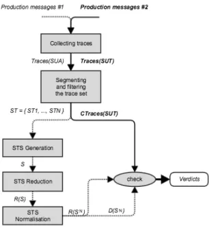
Figure 1 depicts our framework named Autofunk, which is split into two components. The first one infers models that
Figure 1. Autofunk’s overall architecture
represent the functional behaviours of a system under anal-ysis SUA. We have chosen Symbolic Transition Systems (STS) as models since these are known as very general and powerful formal models for describing several aspects of event-based systems.
Autofunk’s model generator is mainly framed upon an inference engine to lift in abstraction the production mes-sages and to build STSs by means of successive transforma-tions. Human expert knowledge has been transcribed with inference rules following this pattern: When condition, Then action(s). These help filter and format production messages. A machine learning technique is then used to automatically remove undesired behaviours, and to cluster production messages into the trace sets ST1, ..., STn, one set for each
entry point of the system. Next, it infers the model S, which corresponds to the list of STSs S = {S1, ..., Sn}, from these
trace sets by means of STS based inference rules. Last but not least, the STSs are reduced in size to be more easily manipulated. Indeed, the first STSs may include thousands and thousands of states, which may lead to a state space explosion problem when using them for testing.
The second part of Autofunk takes production messages as input from another system under test SUT , and checks whether SUT conforms with SUA. We propose two im-plementation relations to define the notion of conformance between the observable behaviours of SUA with those of SU T.
In the next section, we briefly recall how STS models are inferred by Autofunk, since this part has already been presented in [20]. Then, we detail the passive testing com-ponent.
IV. MODEL INFERENCE FOR INDUSTRIAL SYSTEMS
Given a system SUA and a set of production messages, Autofunk builds the model S = {S1, ..., Sn} such that each
Si is an exact model describing the functional behaviours of
a production line in the system SUA. A. Models as STS
Before introducing the model inference module of Auto-funk, we briefly give some definitions related to the STS model below, but we refer to [7] for a more extensive description.
Definition 1 (Variable assignment) We assume that there exist a domain of values denoted D and a variable set X taking values in D. The assignment of variables in Y ✓ X to elements of D is denoted with a mapping ↵ : Y ! D. ↵(x)denotes the assignment of the variable x 2 D. Definition 2 (STS) A Symbolic Transition System (STS) is a tuple < L, l0, V, V0, I, ⇤,!>, where:
• STSs do not havestates but locations (a.k.a. symbolic
states), and L is the finite location set, with l0 being
the initial one,
• V is the finite set of internal variables, while I is
the finite set of parameters. The internal variables are initialised with the condition V0 on V ,
• ⇤ is the finite set of symbolic actions a(p) (a being
a symbol), with p = (p1, . . . , pk) a finite set of
parameters in Ik(k2 N),
• ! is the finite transition set. A transition
(li, lj, a(p), G, A), from the location li 2 L to
lj 2 L, also denoted li
a(p),G,A
! lj, is labelled by:
– an action a(p) 2 ⇤,
– a guard G over (p [ V ), which restricts the firing of the transition. We consider guards written with conjunctions of equalities: ^
x2I[V
(x == val), – internal variables that are updated with the
as-signment function A of the form (x := Ax)x2V,
Ax being an expression over p [ V .
Notation: we also denote P rojx(G)the projection of the
guard G over the variable x 2 I [ V , which extracts the equality (x == val) from G. For example, given the guard G1= [nsys == 1^ nsec == 8 ^ point == 1 ^ pid == 1],
P rojnsys(G1) = (nsys == 1). For readability purpose, if
A is the identity function idV, we denote a transition with
li a(p),G
! lj. We also use the generalised transition relation
) to represent STS paths: l (a1,G1,A1)...(an,Gn,An) ===============) l0= def 9l0. . . ln, l = l0 a1,G1,A1 ! l1. . . ln 1 an,Gn,An ! ln= l0.
A STS is also associated with a LTS (Labelled Transition System) to formulate its semantics. The LTS semantics corresponds to a valued automaton without any symbolic
1 17 Jun 2014 23 : 2 9 : 5 9 . 0 0 | INFO |New F i l e
3 17 Jun 2014 23 : 2 9 : 5 9 . 5 0 | 1 7 0 1 1 |MSG IN [ n s y s : 1] [ n s e c : 8 ] [ p o i n t : 1 ] [ p i d : 1 ] 5 17 Jun 2014 23 : 2 9 : 5 9 . 6 1 | 1 7 0 2 1 |MSG OUT [ n s y s : 1] [ n s e c : 8 ] [ p o i n t : 3 ] [ t p o i n t : 8 ] [ p i d : 1 ] 7 17 Jun 2014 23 : 2 9 : 5 9 . 7 0 | 1 7 0 1 1 |MSG IN [ n s y s : 1] [ n s e c : 8 ] [ p o i n t : 2 ] [ p i d : 2 ] 9 17 Jun 2014 23 : 2 9 : 5 9 . 9 2 | 1 7 0 2 1 |MSG OUT [ n s y s : 1] [ n s e c : 8 ] [ p o i n t : 4 ] [ t p o i n t : 9 ] [ p i d : 2 ]
Figure 2. An example of production messages
variables, which is often infinite: the LTS states are la-belled by internal variable assignments, and transitions are labelled by actions associated with parameter assignments. The semantics of a STS S =< L, l0, V, V 0, I, ⇤, !> is the LTS ||S|| =< Q, q0,P,!> composed of valued states in
Q = L⇥ DV, q0= (l0, V 0)is the initial one,Pis the set
of valued symbols, and ! is the transition relation. Intuitively, for a STS transition l1
a(p),G,A
! l2, we obtain
a LTS transition (l1, v) a(p),↵
! (l2, v0)with v an assignment
over the internal variable set if there exists a parameter value set ↵ such that the guard G evaluates to true with v[↵. Once the transition is fired, the internal variables are assigned with v0 derived from the assignment A(v [ ↵).
Finally, runs and traces, which represent executions and event sequences, can also be derived from LTS semantics: Definition 3 (Runs and traces) Given a STS S = < L, l0, V, V0, I, ⇤,!>, interpreted by its LTS semantics
||S|| =< Q, q0,P,!>, a run q0↵0...↵n 1qn is an
al-ternate sequence of states and valued actions. Run(S) = Run(||S||) is the set of runs found in ||S||.
It follows that a trace of a run r is defined as the projection projP(r) on the actions. T races
F(S) =
T racesF(||S||), with F ✓ L is the set of traces of all runs
finished by states in F DV.
We are now ready to present the different steps to infer models from an industrial system SUA. More details are available in [20].
B. Production messages and traces
Autofunk takes production messages as input from a system under analysis SUA. A production message is mainly compound of a label along with kinds of variable assignments. An example of messages is given in Figure 2. For instance, 17011 is a label and [point : 1] can be seen as a variable assignment.
Production messages are transformed no matter their initial source, so that it is possible to use data from dif-ferent providers. To avoid disrupting the (running) system under analysis SUA, we do not instrument the production
equipments composing the whole system. Everything is done offline with a logging system or with monitoring. Production messages are then formatted, filtered, and reconstructed as traces by means of inference rules. A trace represents the behaviour observed from SUA against one product, i.e. tires in our context, which are numbered with an identifier pid. We call the resulting trace set T races(SUA):
Definition 4 (Production system traces) Given a system under analysis SUA, T races(SUA) denotes its format-ted trace set. T races(SUA) includes traces of the form (a1, ↵1) . . . (an, ↵n)such that (ai, ↵i)(1in)are (ordered)
valued actions having the same identifier assignment over the variable pid.
C. Trace segmentation and filtering
We define a complete trace as a trace containing all valued actions expressing the path taken by a product in a production system, from the beginning, i.e. one of its entry points, to the end, i.e. one of its exit points. In the trace set T races(SU A), we do not want to keep incomplete traces, i.e. traces that do not express entire behaviours of products on production lines.
The trace set T races(SUA) is analysed with a machine learning technique to segment it into several subsets, one per entry point of the system SUA. We leverage this process to also remove incomplete traces, i.e. traces that do not express an execution starting from an entry point and ending to an exit point. These can be extracted by analysing the traces and the variable point, which captures the product physical location.
Definition 5 (Complete traces) Let SUA be a system un-der analysis and T races(SUA) be its trace set. A trace t = a1(↵1)...an(↵n) 2 T races(SUA) is said complete iff
↵1 includes an assignment point = val, which denotes an
entry point of SUA and ↵nincludes an assignment point =
val, which denotes an exit point. The complete traces of SU Aare denoted with CT races(SUA) ✓ T races(SUA). In order to determine the entry and exit points of SUA, we rely on an outlier detection approach [21]. An outlier is an observation which deviates so much from the other observations as to arouse suspicions that it was generated by a different mechanism. More precisely, we chose to use the k-means clustering method, a machine learning algorithm, which is both fast and efficient, and does not need to be trained before being effectively used (that is called unsuper-vised learning, and it is well-known in the machine learning field). k-means clustering aims to partition n observations into k clusters. Here, observations are represented by the variable point present in each trace of T races(SUA), which captures the product physical location, and k = 2 as we want to group the outliers together, and leave the other points in
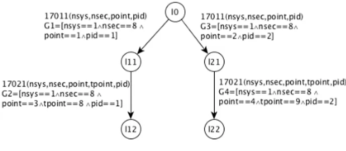
Figure 3. First generated model (STS)
another cluster. But, since we want to leverage the largest part of the initial trace set, we apply k-means clustering several times until reaching 80% of traces retained. Once, the entry and exit points are found, we segment T races(SUA) and obtain a set CT races(SUA) = {ST1, . . . , STn}.
D. STS generation
Given a trace set STi2 CT races(SUA), the STS
gener-ation is done by transforming traces into runs, and runs into STSs. The translation of STiinto a run set denoted Runsiis
done by completing traces with states. All the runs of Runsi
have states that are unique except for the initial state (l0, V0)
with V0=; an initial empty condition. We defined such a set
to ease the process of building a STS having a tree structure. Runs are transformed into STS paths that are assembled together by means of a disjoint union. The resulting STS forms a tree compound of branches starting from the location l0. Parameters and guards are extracted from the assignments found in valued actions. Considering the complete trace sets CT races(SU A) ={ST1, . . . , STn}, we obtain the model
S={S1, . . . , Sn}.
Rather than giving the formal transformation of trace sets into STSs (we refer to [20]), we propose to show its functioning with the example of Figure 2. Production messages are translated into the following complete traces: CT races(SU A) = {(17011(nsys = 1, nsec = 8, point = 1, pid = 1) 17021(nsys = 1, nsec = 8, point = 3, tpoint = 8, pid = 1)), (17011(nsys = 1, nsec = 8, point = 2, pid = 2) 17021(nsys = 1, nsec = 8, point = 4, tpoint = 9, pid = 2))}.
These traces are then transformed into runs by injecting new states between the valued actions, except for the initial state (l0, V0), which is unique. Variable assignments are
translated into guards that are conjunctions of equalities, and STS locations are derived from states. We obtain the STS of Figure 3, which includes all the labels and assignments of the original production messages. One can also notice that such a STS is not an approximation as each of its paths captures an execution of SUA.
E. STS reduction
The STS models Si of S = {S1, . . . , Sn}, are usually too
large, and thus cannot be beneficial as is. That is why our framework adds a reduction step, aiming at diminishing the first model into a second one, denoted R(Si) that will be
more usable.
This step can be seen as a formal classification method (data mining) which consists in combining STS paths that have the same sequences of STS actions, so that we still obtain a model having a tree structure. When paths are combined together, parameter assignments are wrapped into matrices in such a way that trace equivalence between the first model and the new one is preserved. The use of matrices offers another advantage: the parameter assignments are now packed into a structure that can be more easily analysed or leveraged later on.
Given a STS Si, this adaptation is achieved by two steps.
Every path of Si is adapted to express sequences of guards
in a vector form. Then, the concatenation of these vectors gives birth to matrices. The first step is done by means of the STS operator Mat. For simplicity purpose, we do not provide the definition here, but we refer to [20]. In short, for each path b of Si, this operator collects the list of guards
(G1, . . . , Gn)found in the transitions of b, and stores it in
a vector denoted Mat(b). It results in a new STS Mat(Si)
composed of transitions of the form l aj(pj),M at(b)[j],Aj ! l0.
Thereafter, the STS paths of Mat(Si), which have the
same sequences of actions, are assembled: these paths can be recognised by means of an equivalence relation over STS paths from which equivalence classes can derived:
Definition 6 (STS path equivalence class) Let Si =<
LSi, l0Si, VSi, V 0Si, ISi, ⇤Si,!Si>be a STS obtained from CT races(SU A)and having a tree structure. [b] denotes the equivalence class of paths of Si such that:
[b] = {bj = l0Si (a1(p1),G1j,A1j)...(am(pm),Gmj,Amj) ========================) lmj(j > 1)2!m(Si)| b = l0Si (a1(p1),G1,A1)...(am(pm),Gm,Am) ======================) lm}
The reduced STS denoted R(Si)of Si is finally obtained
by concatenating all the paths of each equivalence class [b] found in Mat(Si)into a single path. The vectors found in
the paths of [b] are concatenated as well into the same unique matrix M[b]. A column of this matrix represents a complete
and ordered sequence of guards found in one initial path of Si. R(Si)is defined as follows:
Definition 7 Let Si =< LSi, l0Si, VSi, V 0Si, ISi, ⇤Si, !Si> be a STS inferred from a structured trace set
T races(SU A). The reduction of Si is modelled by the STS
R(Si) =< LR, l0R, VR, V 0R, IR, ⇤R,!R>where: • l0R= l0M at(Si), IR= IM at(Si), ⇤R= ⇤M at(Si),
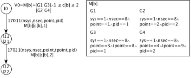
Figure 4. Reduced model (STS)
• LR, VR, V 0R,!R are defined by the following
infer-ence rule: [b] ={b1, . . . , bm} b = l0Si (a1(p1),G11,A11)...(an(pn),Gn1,An1) =======================)M at(Si)ln V 0R:= V 0R^ M[b]= [M at(b1), . . . , M at(bm)]^ (1 c[b] m), l0R
(a1(p1),M[b][1,c[b]],idV)...(an(pn),M[b][n,c[b]],idV) ================================)!R
(ln1. . . lnm)
A column of the matrix M[b] represents a successive list
of guards found in a path of the initial STS Si. The choice
of the column in a matrix depends on a new variable c[b].
The STS R(Si)has less paths but still expresses the initial
behaviours described by the STS Si. This is captured with
the following proposition:
Proposition 8 Let SUA be a system under analysis and T races(SU A)be its traces set. R(Si)is a STS derived from
T races(SU A). We have T races(R(Si)) = T races(STi)✓
T races(SU A).
We obtain the model R(S) = {R(S1), ..., R(Sn)}. Figure
4 depicts the reduced model obtained from the STS of Figure 3. Now we have only one path where guards are packed into one matrix M[b].
F. STS normalisation
Both models S and R(S) include parameters that are dependent to the products being manufactured. That is a consequence of generating models that describe behaviours of a continuous stream of products which are strictly iden-tified, i.e. for each action in a given sequence, we have the assignment (pid = val) (pid stands for product identifier). Here, we normalise these models before using them for testing. The resulting models are denoted with SN and
R(SN). In short, we remove the assignments relative to
product identifiers and timestamps. Furthermore, we label all the final locations with ”Pass”. We denote these locations as verdict locations and gather them in the set P ass ✓ LSN. Both SN and R(SN)represent more generic models, i.e. they
express some possible behaviours that should happen. These behaviours are represented by the traces T racesP ass(SN) =
[
1in
T racesP ass(SNi ) = T racesP ass(R(SN)).
We refer to these traces as pass traces. We call the other traces possibly fail traces.
V. OFFLINE PASSIVE TESTING
We consider both models SN and R(SN)of a system
un-der analysis SUA, generated by our inference-based model generation framework, as reference models. In this section, we present the second part of our framework, dedicated to the passive testing of a system under test SUT . As depicted in Figure 1, the passive testing of SUT is performed offline, i.e. a set of production messages has been collected beforehand from SUT , in the same way as for SUA. These are grouped into traces to form the trace set T races(SUT ). The later is filtered as described in Section IV-C to obtain a set of complete traces denoted with CT races(SUT ). We then perform passive testing to check if SUT conforms to SN. Below, we define conformance with implementation
relations, and provide a passive testing algorithm that aims to check whether these relations hold.
A. Implementation relations and verdicts
Our industrial partner wishes to check whether every complete execution trace of SUT matches a behaviour captured by SN. In this case, the test verdict must reflect
a successful result. On the contrary, if an execution of SUT is not captured by SN, one cannot conclude that SUT
is faulty because SN is a partial model, and it does not
necessarily includes all the correct behaviours. Below, we formalise theses verdict notions with two implementation relations. Such relations between models can only be written by assuming the following classical test assumption: the black-box system SUT can be described by a model, here with a LTS (see Definition 2). We also denote this model with SUT .
The first implementation relation, denoted with ct, refers
to the trace preorder relation [8]. It aims at checking whether all the complete execution traces of SUT are pass traces of SN =
{SN
1, ..., SNn}. The first implementation relation can
be written with:
Definition 9 Let SN be an inferred model of SUA and
SU T be the system under test. When SUT produces com-plete traces also captured by SN, we write:
SU T ctSN =def CT races(SU T )✓ T racesP ass(SN)
Pragmatically, the reduced model R(SN) sounds more
convenient for passively testing SUT since it is strongly reduced in terms of size compared to SN. The test relation
can also be written as below since both models SN and
R(SN)are trace equivalent (Proposition 8):
Proposition 10 SUT ct SN iff CT races(SUT ) ✓
T racesP ass(R(SN))
As stated previously, the inferred model SN of SUA
is partial, and might not capture all the behaviours that should happen on SUT . Consequently, our partner wants a weaker implementation relation, which is less restrictive on the traces that should be observed from SUT . Intuitively, this second relation aims to check that, for every complete trace t = a1(↵1)...am(↵m) of SUT , we also have a set
of traces of T racesP ass(SN)having the same sequence of
symbols such that every variable assignment ↵j(x)(1jm)
of t is found in one of the traces of T racesP ass(SN)
with the same symbol aj. If we take back the example
of Figure 3, the trace t = (17011(nsys = 1, nsec = 8, point = 1, pid = 1) 17021(nsys = 1, nsec = 8, point = 4, tpoint = 9, pid = 1) is not a pass trace of SN because
this trace cannot be extracted from one of the paths of the STS of Figure 3, on account of the variables point and tpoint, which do not take the expected values. However, both variables are assigned with point = 4, tpoint = 9 in the second path. The second implementation relation aims at expressing that this trace t captures a correct behaviour as well.
This implementation relation, denoted with mct, is
writ-ten with:
Definition 11 Let SN be an inferred model of SUA
and SUT be the system under test. We denote SU T mct SN =def 8t = a1(↵1)...am(↵m) 2
CT races(SU T ),8↵j(x)(1jm),9SNi 2 SN and t0 2
T racesP ass(SNi ) such that t0 = a1(↵01)...am(↵0m) and
↵0
j(x) = ↵j(x)
In the following, we rewrite this relation in an equivalent but simpler form. According to the above definition, the successive symbols and variable assignments of a trace t 2 CT races(SUT ) must be found into several traces of T racesP ass(SNi ), which have the same sequence of
symbols a1...am as the trace t. The reduced model R(SNi )
was previously constructed to capture all these traces in T racesP ass(SNi ), having the same sequence of symbols.
Indeed, given a STS SN
i , all the STS paths of SNi , which
have the same sequence of symbols labelled on the transi-tions, are compacted into one STS path b in R(SN
i )whose
transition guards are stored into a matrix M[b]. Given a trace
a1(↵1)...am(↵m) 2 CT races(SUT ) and a STS path b of
R(SN
i ) having the same sequence of symbols a1...am, the
relation can be now formulated as follows: for every valued action aj(↵j), each variable assignment ↵j(x)must satisfies
at least one of the guards of the matrix line j in M[b][j,⇤].
The implementation relation mct can then be written
with:
Proposition 12 SUT mctSN iff 8t = a1(↵1)...am(↵m)
2 CT races(SUT ), 9R(SN
i )2 R(SN ) and b = l0R(SN i )
(a1(p1),M[b][1,c[b]]),...,(am(pm),M[b][m,c[b]]) ============================) lm
with (1 c[b] k) such that 8↵j(x)(1 j m), ↵j(x)|=
M[b][j, 1]_ ... _ M[b][j, k]and lm2 P ass
The disjunction of guards M[b][j, 1]_..._M[b][j, k], found
in the matrix M[b], could be simplified by gathering all the
equalities x == val together with disjunctions for every variable x 2 pj. Such equalities can be extracted with the
Proj operator (see Definition 2). We obtain one guard of the formVx2pj(x == val1_..._x == valk). The STS D(SNi ),
derived from R(SN
i ), is constructed with this simplification
of guards: Definition 13 Let R(SN i ) =< LR, l0R, VR, V 0R, IR, ⇤R, !R> be a STS of R(SN). We denote D(SNi ) the STS < LD, l0D, VD, V 0D, ID, ⇤D,!D> derived from R(SNi ) such that: • LD= LR, l0D= l0R, ID= IR, ⇤D= ⇤R,
• VD, V 0Dand !D are given by the following inference
rule: b = l0R (a1(p1),M[b][1,c[b]])...(am(pm),M[b][m,c[b]] ==========================)!R lm (1 c[b] k) in V 0R l0D (a1(p1),Mb[1])...(am(pm),Mb[m]) =====================)!D lm V 0D= V 0D^ Mb, Mb[j](1jm)= ^ x2pj (P rojx(M[b][j, 1])_ · · · _ P rojx(M[b][j, k]))
D(SN)denotes the model {D(SN
1 ), ..., D(SNn)}.
The second implementation relation mct can now be
expressed by:
Proposition 14 SUT mctSN iff 8t = a1(↵1)...am(↵m)
2 CT races(SUT ), 9D(SN i )2 D(SN)and l0D(SN i ) (a1(p1),G1),...,(am(pm),Gm) ==================) lm such that 8↵j(1 j m), ↵j |= Gj and lm2 P ass.
cmt now means that a trace of SUT must also be a
pass trace of the model D(SN) = (D(SN
1 ), ..., D(SNn)).
Furthermore, this notion of trace inclusion can be formulated with the first implementation relation ct as follows:
Proposition 15 SUT mct SN iff CT races(SUT ) ✓
T racesP ass(D(SN))
SU T mct SN , SUT ctD(SN)
The implementation relation mct is now expressed with
the first relation ct, which implies that our passive testing
algorithm shall be the same for both relations but shall take different reference models.
B. Passive testing algorithm
The passive testing algorithm, which aims to check whether the two previous implementation relations hold, is given in Algorithm 1. It takes the complete traces of SU T and the models R(SN) and D(SN), with regards to
Propositions 10 and 15. It returns the verdict ”Passct”
(”Passmct”) if the relation ct is satisfied (mct
respec-tively).
It relies upon the function checktrace(trace t, STS S) to check whether the trace t = a1(↵1)...am(↵m)is also a trace
of the STS S. If a STS path b is composed of the same sequence of symbols as the trace t, the function tries to find a matrix column M = M[b][⇤, i] such that every variable
assignment ↵j satisfies the guard M[j]. If such a column of
guards exists, the function returns True, and False otherwise. Algorithm 1 covers every trace t of CT races(SUT ) and tries to find a STS R(SN
i )such that t is also a trace of R(SNi )
with check(t, R(SN
i )). If no model R(SNi )has been found,
the trace t is placed into the set T1. T1 gathers the possibly
fail traces w.r.t. ct. Thereafter, the algorithm performs the
same step but on the STS D(SN). One more time, if no
model D(SN
i )has been found, the trace t is placed into the
set T2. The later gathers the possibly fail traces, w.r.t. the
relation mct.
Finally, if T1 is empty, the verdict ”Passct” is returned,
which means that the first implementation relation holds. Otherwise, T1 is provided. If T2 is empty, the verdict
”Passmct” is returned, or T2in the other case.
When one of the implementation relations does not hold, this algorithm offers the advantage to provide the possibly fail traces of CT races(SUT ). Such traces can be later analysed to check if SUT is correct or not. That is helpful for Michelin engineers as it allows them to only focus on what are potentially faulty behaviours, reducing debugging time, and making engineers more efficient.
VI. EVALUATION
We conducted several experiments with real sets of pro-duction messages, recorded in one of Michelin’s factories at different periods of time. We executed our implementation on a Linux (Debian) machine with 12 Intel(R) Xeon(R) CPU X5660 @ 2.8GHz and 64GB RAM.
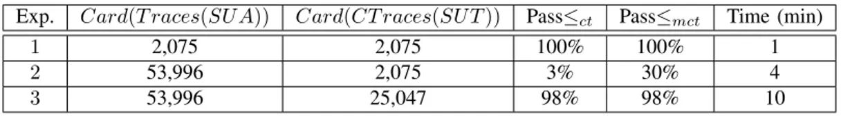
We present, in Figure 5, the results of several experiments on the same production system with different trace sets, recorded at different periods of time. We focus on the passive testing component here, but one can find an extensive evaluation on the model inference part in [20]. The first column shows the experiment number, columns 2 and 3 respectively give the sizes of the trace sets of the system under analysis SUA and of the system under test SUT . The two next columns show the percentage of pass traces w.r.t the relations ct and mct. The last column indicates
Exp. Card(T races(SU A)) Card(CT races(SU T )) Passct Passmct Time (min)
1 2,075 2,075 100% 100% 1
2 53,996 2,075 3% 30% 4
3 53,996 25,047 98% 98% 10
Figure 5. Results of our testing method based on a same specification
Algorithm 1: Passive testing algorithm
input : R(SN ) ={R(SN 1), ..., R(S N n)}, D(S N ) = {D(SN 1), ..., D(SNn)}, CT races(SUT )
output: Verdits or possibly fail trace sets T1, T2 1 T1= T2=;;
2 foreach t 2 CT races(SUT ) do 3 foreach i 2 1, . . . , n do
4 if check (t, R(SNi ))then break ; 5 if i == n then
6 T1= T1[ {t} 7 foreach i 2 1, . . . , n do
8 if check (t, D(SNi ))then break ; 9 if i == n then T2= T2[ {t} ; 10 if T1==; then return ”Passct”; 11 else return T1;
12 if T2==; then return ”Passmct”; 13 else return T2;
14 Function check(trace t, STS S ) : bool is
15 if 9b = l0S=========================(a1(p1),G1,A1)...(an(pn),Gn,An)) ln|trace =
(a1, ↵1), . . . , (an, ↵n)and ln2 P ass then 16 M[b]= M at(b)is the Matrix k ⇥ m of b; 17 i = 1;
18 while i m do 19 M = M[b][⇤, i]; 20 foreach j 2 1, . . . , n do 21 if ↵j6|= M[j] then break ; 22 if j == n then return T rue ; 23 i + +;
24 return F alse;
In Experiment 1, we decided to use the same production messages for both inferring models, i.e. specifications, and testing. This experiment shows that our implementation behaves correctly when trace sets are similar, i.e. when behaviours of both SUA and SUT are equivalent.
Experiment 2 has been run with traces of SUT that are older than those of SUA, which is unusual as the defacto usage of our framework is to build specifications from a production system SUA, and to take a newer or updated system as SUT . Here, only 30% of the traces of SUT are pass traces w.r.t. the second implementation relation (same sequence of symbols with different values). There are two explanations: the system has been updated between the two periods of record (4 months), and production campaigns, i.e. grouping of planned orders and process orders to produce a certain amount of a products over a certain period of time, were different (revealed by Autofunk, indicating that values for some key parameters were unknown).
Finally, experiment 3 shows good results as the specification
models are rich enough, i.e. built from a larger set of traces (10 days) than the one collected on SUT . Such an experi-ment is a typical usage of our framework at Michelin. The traces of SUT have been collected for 5 days, and it took only 10 minutes to check conformance. While 98% of the traces are pass traces, the remaining 2% are new behaviours that never occured before. Such information are essential for Michelin engineers so that they can determine the root causes (for instance, one trace was a manual intervention made by an operator).
VII. CONCLUSION
This paper presents Autofunk, a fast passive testing frame-work combining different fields such as model inference, expert systems, and machine learning. First, given a large set of production messages, our framework infers exact models whose traces are included in the initial trace set of a system under analysis. Such models are then reused as specifications to perform offline passive testing, using a second set of traces recorded on a system under test. Using two implementation relations, Autofunk is able to determine what has changed between the two systems. This is particularly useful for our industrial partner Michelin since potential regressions can be detected before deploying changes in production.
Technical improvements put aside, we plan to work on online passive testing in the future, enabling just-in-time fault detection. In short, we plan to record traces on a system under test on the fly, and to check whether those traces satisfy specifications still generated from a system under analysis. One additional need, directly related to our industrial partner Michelin, is to be able to focus on specific locations of a workshop, rather than on the whole workshop, because some parts are more critical than others. The combination of both enhancements on our framework should bring significant improvements to end users.
REFERENCES
[1] A. Memon, I. Banerjee, and A. Nagarajan, “Gui ripping: Reverse engineering of graphical user interfaces for testing,” in Proceedings of the 10th Working Conference on Reverse Engineering, ser. WCRE ’03. Washington, DC, USA: IEEE Computer Society, 2003, pp. 260–. [Online]. Available: http://dl.acm.org/citation.cfm?id=950792.951350
[2] A. Mesbah, A. van Deursen, and S. Lenselink, “Crawling Ajax-based web applications through dynamic analysis of user interface state changes,” ACM Transactions on the Web (TWEB), vol. 6, no. 1, pp. 3:1–3:30, 2012.
[3] P. Tonella, C. D. Nguyen, A. Marchetto, K. Lakhotia, and M. Harman, “Automated generation of state abstraction functions using data invariant inference,” in 8th International Workshop on Automation of Software Test, AST 2013, San Francisco, CA, USA, May 18-19, 2013, 2013, pp. 75–81. [Online]. Available: http://dx.doi.org/10.1109/IWAST.2013. 6595795
[4] H. Hungar, T. Margaria, and B. Steffen, “Model generation for legacy systems,” in Radical Innovations of Software and Systems Engineering in the Future, 9th International Workshop, RISSEF 2002, Venice, Italy, October 7-11, 2002, Revised Papers, ser. Lecture Notes in Computer Science, M. Wirsing, A. Knapp, and S. Balsamo, Eds., vol. 2941. Springer, 2002, pp. 167–183. [Online]. Available: http://dx.doi.org/10.1007/978-3-540-24626-8 11
[5] W. Choi, G. Necula, and K. Sen, “Guided gui testing of android apps with minimal restart and approximate learning,” in Proceedings of the 2013 ACM SIGPLAN International Conference on Object Oriented Programming Systems Languages and Applications, ser. OOPSLA ’13. New York, NY, USA: ACM, 2013, pp. 623–640. [Online]. Available: http://doi.acm.org/10.1145/2509136.2509552 [6] D. Amalfitano, A. R. Fasolino, P. Tramontana, B. D. Ta, and
A. M. Memon, “Mobiguitar – a tool for automated model-based testing of mobile apps,” IEEE Software, 2014. [7] L. Frantzen, J. Tretmans, and T. Willemse, “Test Generation
Based on Symbolic Specifications,” in FATES 2004, ser. Lec-ture Notes in Computer Science, J. Grabowski and B. Nielsen, Eds., no. 3395. Springer, 2005, pp. 1–15.
[8] R. D. Nicola and M. Hennessy, “Testing equivalences for processes,” Theoretical Computer Science, vol. 34, pp. 83 – 133, 1984.
[9] D. Lorenzoli, L. Mariani, and M. Pezz`e, “Automatic generation of software behavioral models,” in Proceedings of the 30th International Conference on Software Engineering, ser. ICSE ’08. New York, NY, USA: ACM, 2008, pp. 501–510. [Online]. Available: http://doi.acm.org/10.1145/ 1368088.1368157
[10] L. Mariani and F. Pastore, “Automated identification of failure causes in system logs,” in Software Reliability Engineering, 2008. ISSRE 2008. 19th International Symposium on, Nov 2008, pp. 117–126.
[11] V. Dallmeier, C. Lindig, A. Wasylkowski, and A. Zeller, “Mining object behavior with adabu,” in Proceedings of the 2006 International Workshop on Dynamic Systems Analysis, ser. WODA ’06. New York, NY, USA: ACM, 2006, pp. 17–24. [Online]. Available: http://doi.acm.org/10.1145/ 1138912.1138918
[12] J. H. Andrews and Y. Zhang, “Broad-spectrum studies of log file analysis,” in Proceedings of the 22nd International Conference on Software Engineering (ICSE 2000), 2000. [13] D. Cotroneo, R. Pietrantuono, L. Mariani, and F. Pastore,
“Investigation of failure causes in workload-driven reliability testing,” in Fourth international workshop on Software qual-ity assurance: in conjunction with the 6th ESEC/FSE joint meeting. ACM, 2007, pp. 78–85.
[14] L. Mariani and M. Pezze, “Dynamic detection of cots com-ponent incompatibility,” IEEE Software, vol. 24, no. 5, pp. 76–85, 2007.
[15] M. Salah, T. Denton, S. Mancoridis, and A. Shokouf, “Sce-nariographer: A tool for reverse engineering class usage scenarios from method invocation sequences,” in In ICSM. IEEE Computer Society, 2005, pp. 155–164.
[16] M. Pradel and T. R. Gross, “Automatic generation of object usage specifications from large method traces,” in Proceed-ings of the 2009 IEEE/ACM International Conference on Automated Software Engineering, ser. ASE ’09. Washington, DC, USA: IEEE Computer Society, 2009, pp. 371–382. [17] S. Anand, M. Naik, M. J. Harrold, and H. Yang, “Automated
concolic testing of smartphone apps,” in Proceedings of the ACM SIGSOFT 20th International Symposium on the Foundations of Software Engineering, ser. FSE ’12. New York, NY, USA: ACM, 2012, pp. 59:1–59:11. [Online]. Available: http://doi.acm.org/10.1145/2393596.2393666 [18] S. Artzi, A. Kiezun, J. Dolby, F. Tip, D. Dig, A. Paradkar, and
M. Ernst, “Finding bugs in web applications using dynamic test generation and explicit-state model checking,” Software Engineering, IEEE Transactions on, vol. 36, no. 4, pp. 474– 494, 2010.
[19] D. Angluin, “Learning regular sets from queries and counterexamples,” Information and Computation, vol. 75, no. 2, pp. 87 – 106, 1987. [Online]. Available: http://www. sciencedirect.com/science/article/pii/0890540187900526 [20] S. Salva and W. Durand, “Industry paper: Autofunk, a fast and
scalable framework for building formal models from produc-tion systems.” in Proceedings of the 9th ACM Internaproduc-tional Conference on Distributed Event-Based Systems, DEBS ’15, Oslo, Norway, June 29 - July 3, 2015. ACM, 2015. [21] V. J. Hodge and J. Austin, “A Survey of Outlier Detection
Methodologies,” Artificial Intelligence Review, vol. 22, pp. 85–126, 2004.