Dark energy and CMB anisotropy

Dark Energy and CMB Anisotropy

by

Yukyan Lam

Submitted to the Department of Physics

in partial fulfillment of the requirements for the degree of

Bachelor of Science in Physics

at the

MASSACHUSETTS INSTITUTE OF TECHNOLOGY

June 2004

() Massachusetts Institute of Technology 2004. All rights reserved.

Author.

...

...

...

(1

/

C-

Department of Physics

May 14, 2004

Certified

by ...

...

Edmund Bertschinger

Department of Physics

Thesis Supervisor

Accepted by ...

... .

David Pritchard

Senior Thesis Coordinator, Department of Physics

MASSACHUSETTS INSTITUTE OF TECHNOLOGY ..

''

-'- R. IES _ARCHIVES JUL 0 7 2004 I iI I I II L ' -I

Dark Energy and CMB Anisotropy

by

Yukyan Lam

Submitted to the Department of Physics

on May 14, 2004, in partial fulfillment of the requirements for the degree of

Bachelor of Science in Physics

Abstract

According to the WMAP and earlier COBE observations, the Cosmic Microwave Background (CMB) anisotropy power on large angular scales appears to be signif-icantly lower than predicted by the standard model of cosmology. We propose a

scalar field model of the dark energy as a mechanism for suppressing low I multipoles

through late-Universe evolution of metric fluctuations and the integrated Sachs-Wolfe

(ISW) effect. We find that for a constant dark energy equation of state, theoretical

predictions actually give a larger (instead of a desired smaller) value of the quadrupole and other low 1 multipoles.

Thesis Supervisor: Edmund Bertschinger Title: Department of Physics

Acknowledgments

I would like to thank Professor Ed Bertschinger for his devotion to both research and teaching. His dedication has made this thesis not only possible, but a truly memorable

and rewarding experience. I would also like to thank Professor Paul Schechter for his sage advice and continued support in this research process, my undergraduate experience at MIT, and beyond.

Contents

1 Introduction

1.1 The low quadrupole problem-two puzzles in one problem? ... 1.2 Proposed solutions ...

1.3 Perturbed Robertson-Walker spacetime ...

2 Scalar field energy and dynamics

2.1 Mechanics of the scalar field ...

2.2 Stress-energy tensor ... 2.3 Dark energy fluid properties ...

3 Fluid equations

3.1 Stress-energy tensor revisited ... 3.2 Cold dark matter ... 3.3 Dark energy ...

3.4 Total stress-energy variables ...

4 Gravity

4.1 Einstein equations ...

4.2 Combining the Einstein and fluid equations .... 4.2.1 Comparison of equations with DeDeo et al.. 4.2.2 Analytic solution for small kT ...

5 Sachs-Wolfe effect

5.1 CMIB anisotropy contributions ...

11 12 13 16 21 21 23 25 27 27 30 30 31 33 . . . .33 . . . .34 . . . .35 . . . .37 39 39

5.2 CMB angular power spectrum ...

6 Results for a simple equation of state 49

7 Conclusions 57

List of Figures

1-1 Figure from the NASA/WMAP Science Team [1]. CMB angular power

spectrum of the fluctuations in the WMAP full-sky map. The solid curve represents the theoretical prediction of the best fit ACDM model, and the shaded band represents the cosmic variance expected for that model. Even with the cosmic variance, the measured quadrupole, C2

has a surprisingly low value, as seen in the top graph ... 19

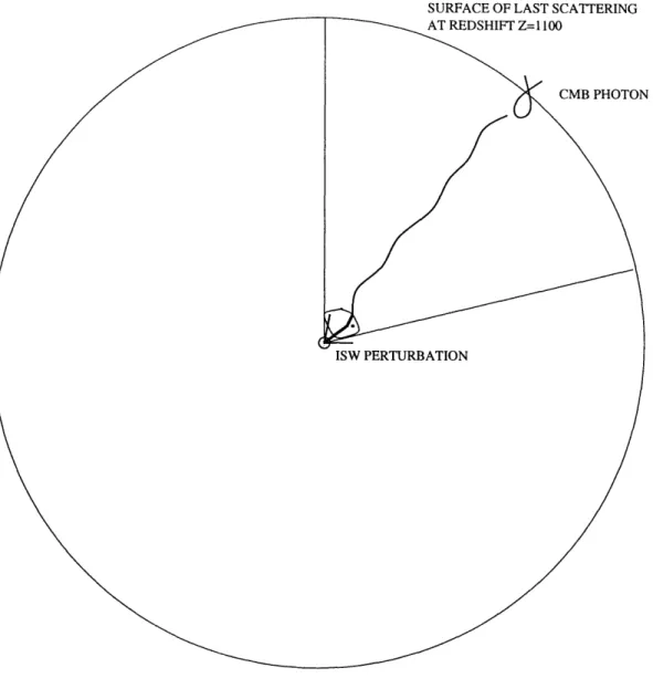
1-2 CMB photon emitted at the surface of last scattering gets "redshifted" by changing gravitational potentials in the foreground ... . 20

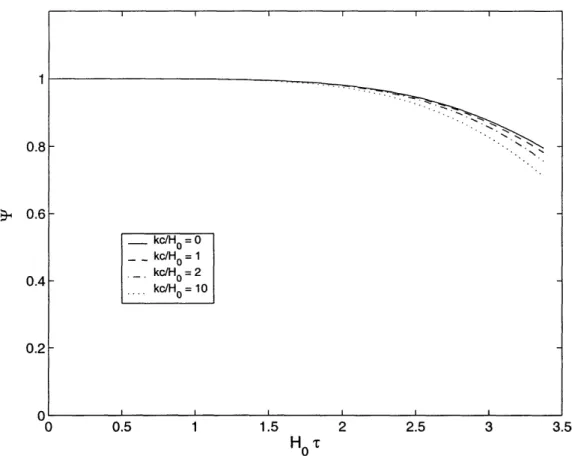
6-1 The evolution of the gravitational perturbation, ', for several different

wavelengths of the perturbations. Here, w4 = -0.8. We see that I

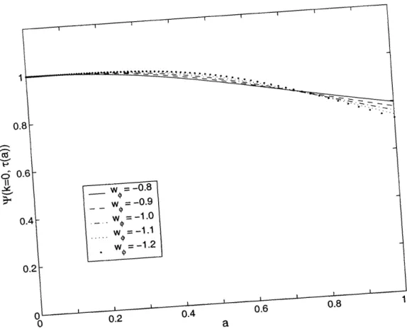
falls off with time, but not very steeply ... 50 6-2 The evolution of the gravitational potential, (k = 0, r(a)), versus a

for various values of wo. We see that in general, T falls off with time. However, when and by how much it falls off depends on the particular value of wo. More negative values of wO lead to greater suppression at

late tim es . . . 51

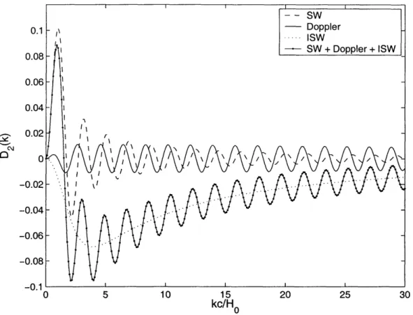
6-3 A plot of D2(k) versus k in units of c/Ho. We used w, = -0.8 for our constant equation of state. The addition of the ISW term lowers the

value of D2(k) but also gives it a greater amplitude. At long wavelength scales (kc/Ho < 10), the ISW term dominates. The Doppler term is

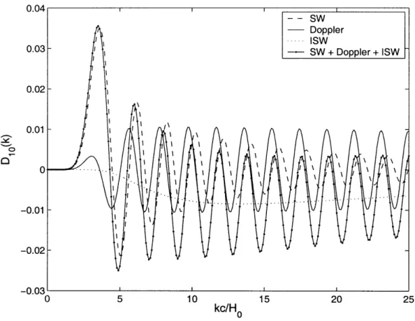
6-4 A plot of D1 0(k) versus k in units of c/Ho. Again, w =-0.8. Here,

the Doppler contribution is important ... 53

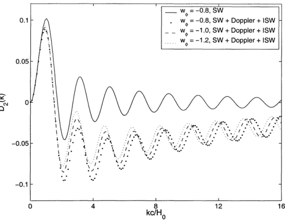
6-5 A plot of D2(k) versus k in units of c/Ho for various values of wo. In

general, the ISW term does not do much to cancel out the SW term,

but the amplitude of D2(k) is smallest for the most negative w. ... . 54

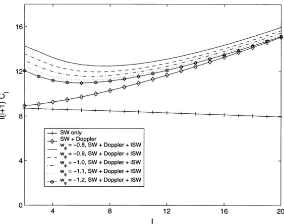
6-6 A plot of theoretically calculated l(l + )Ci versus for various values of wo. The normalization of Cl is based on normalizing the inflationary

power spectrum by k3P = 1. We also plot Cl integrating only the SW term and Cl integrating over only the SW term plus Doppler term. Instead of suppressing Cl, the ISW term increases C ... 55

Chapter 1

Introduction

The two important puzzles in cosmology research today are the Universe's composi-tion and the origin of its structure.

In the classical Big-Bang model of cosmology, the Universe on large scales is

considered to be homogeneous and isotropic. The Cosmic Microwave Background radiation, the light emitted at the surface of last scattering (redshift z = 1100), when first detected in 1965 by Penzias and Wilson seemed to confirm this. The Cosmic Background Explorer (COBE) satellite, launched in 1989, found that there are in fact fluctuations in the radiation temperature, or 'anisotropies', at the level of a few

parts in 100,000. Because the CMB is radiation coming directly from the era of

recombination, these temperature anisotropies give a picture of the earliest cosmic structure formation.

These observations can be tested against the theory-the inflationary theory of the universe. Inflation predicts the initial conditions of the Big Bang, including the temperature perturbations. During inflation, the energy density of the Universe is dominated by the potential of scalar fields and the scale factor is accelerating. Inflation explains why the Universe should be very nearly flat and homogeneous on

large scales.

The Universe is composed of matter and radiation: baryonic matter, dark mat-ter, and radiation. Ordinary, baryonic matter and the cosmic microwave background

significant component of the Universe's energy density is in the form of some

nonbary-onic dark matter. Dark matter neither emits nor absorbs radiation and is therefore

"invisible". But measurement of gravitational lensing effects, for example, can reveal how much dark matter there is in the Universe, where it is, and how it is distributed.

Even taking into account dark matter, however, the Universe's density is still too low-much lower than the critical density required for the nearly flat Universe that we observe. Thus, there is some other "dark energy" component that contributes enough to the energy density to make the Universe flat. Dark energy, with its repulsive gravitational force, is responsible for the acceleration of the expansion of the universe.

In the theories considered so far, the dark energy component takes the form of a

cosmological constant. The standard model of cosmology with the simplest model

of inflation, called ACDM, is a flat, cold dark matter, homogeneous and isotropic cosmological constant-dominated Universe.

1.1 The low quadrupole problem

two puzzles in

one problem?

Inflation predicts the statistical properties of a pattern of temperature fluctuations

that extends all over the sky and varies from place to place. This prediction yields

an angular power spectrum, Cl, that gives the temperature correlation between two

points in the sky 0 ~ 7r/l radians apart. However, recent observations done by the

Wilkinson Microwave Anisotropy Probe (WMAP) team have revealed that on the largest scales, the fluctuations are too smooth for the simplest inflationary model. More specifically, the observed quadrupole moment C2 (and to a lesser extent the

observed octopole moment C3) have values that are anomalously low compared to

the standard model predictions while data from COBE and WMAP fit the standard

models' predictions for the power spectrum extremely well for I > 4 (see Figure 1-1) [1, 2, 3]. Monte Carlo simulations of the observations show that only 0.7% of the standard models would yield a quadrupole as low or lower than the WMAP

quadrupole value [2]. Efstathiou, however, concludes that the posterior probability for the theoretical quadrupole to be as small or smaller than the models' prediction

is about 5% to 10% [4].

In chapter 5, we will show that the angular power spectrum is given by

Cl = 47r / d3k P (k)D2(k).

The first term of the integral, P, (k), deals with the physics of inflation (early Universe physics) and how the Universe was first structured. The second term of the integral involves D (k), the CMB transfer function. It relates the inflationary perturbations to the pattern of CMB temperature anisotropies which includes the actual imprint of fluctuations on the photosphere plus foreground distortions. We will study the fore-ground (late Universe) distortions known as the Integrated Sachs-Wolfe (ISW) effect. They come from the post-recombination contribution to the temperature anisotropies from time-changing gravitational potentials. Matter and energy density contribute to these gravitational potentials and their derivatives, and therefore affect the ISW contribution to the CMB transfer function. Thus, in the equation for the angular power spectrum, C, we incorporate both the physics of structure formation and the

composition of the Universe, which together pose the two main questions in cosmol-ogy.

At the current age of the universe, there seems to be a coincidence that effects of CMB low power (structure) and late-time acceleration caused by dark energy (compo-sition) are both being manifested and becoming important now. One possible solution to the low quadrupole problem probes both: we consider dark energy as a scalar field instead of a cosmological constant and calculate its effect on the quadrupole moment.

1.2 Proposed solutions

Referring back to equation (1.1), we see that if either P(k) or D (k) is modified in some way, or the continuous integral is replaced by a discrete summation (as it

would be in a closed or toroidal universes), then it is possible that the angular power

is lowered.

One solution lies in changing the geometry of the Universe and therefore the nature of the integral [5]. Positively curved (closed) or toroidal (multiply connected)

universes would have a discrete summation with less power at small k and small 1. Simple toroidal models do not work, however [5].

A second solution is proposed in [6], where instead the inflationary power spec-trum of equation (1.1) is changed. Choosing a best-fit cutoff scale, modifications to the inflationary potentials can result in suppression of power at large scales in the

primordial spectrum. Contaldi et al. [6] also propose that a modified ISW

contribu-tion to Di(k) from special models of effective cosmological constant or fluctuacontribu-tions in

the quintessence (dynamical dark energy) field can lead to suppression but have not yet further investigated these possibilities. We examine this latter proposal.

Our solution deals with the late Universe case and a modification to the Integrated

Sachs-Wolfe term arising from the dark energy. Instead of a cosmological constant, the dark energy now takes the form of a scalar field. This new form for the dark

energy, which contributes to energy density and gravity via the Einstein equations, affects the time-evolution of the gravitational potentials present in the ISW term of Dl(k). Thus, late time evolution of the metric fluctuations due to scalar field dark energy might possibly suppress the quadrupole moment through the ISW effect. Furthermore, a modification to the ISW term will change the correlation of two points

in the late Universe and therefore, in looking down the past light cone of photons from

those two directions to the cosmic photosphere, those two points were far apart on the photosphere (see Figure 1-2). Thus, the late Universe modification only affects

the power spectrum of low I values, which is precisely what would be needed to

reconcile the prediction with the measurement and leave the well-matching high

values unchanged.

Thus far, quintessence models with a specific equation of state leading to a partial

suppression through the ISW effect have been considered by DeDeo et al. [7]. They

density) which alter the sound speed. Combined with a specific equation of state,

this can lead to a partial suppression of the angular power spectrum on large scales. However, in this thesis we now consider a simpler class of scalar field models and

examine the equations and solutions in analytical form, as well as their numerical solutions.

In chapter 2, we examine the physics of the scalar field. We begin with the Lagrangian and action of the scalar field. From Hamilton's principle, we obtain an equation of motion for the scalar field. The equation of motion combined with a symmetry principle yields the canonical stress energy tensor. The stress energy tensor has the form of a perfect fluid, and from this, we extract the fluid velocity, pressure, and energy density.

In chapter 3, we examine the fluid equations of dark matter and of dark energy. We get the fluid equations from conservation of the stress energy tensor.

In chapter 4, we consider the contributions of matter and energy (especially includ-ing the scalar field terms) to the gravitational potentials. We present the perturbed Einstein field equations and combine them with the fluid equations for dark matter and dark energy. We get a system of differential equations that can be integrated numerically to give the gravitational potential and its time derivative.

In chapter 5, we derive the CMB transfer function and the CMB angular power spectrum. They are composed of a Sachs-Wolfe term, a Doppler term, and the ISW term. These terms depend on the gravitational potential and its time derivative. The

ISW term is modified by the presence of the dark energy scalar field, which becomes

significant at late times. (The Sachs-Wolfe term and Doppler terms are evaluated at recombination, when the dark energy is insignificant.)

In chapter 6, we show the results found for the gravitational potential, CMB transfer function, and CMB angular power spectrum from numerically integrating the equations in chapters 4 and 5. We consider only the case where the dark energy's equation of state is a constant. We observe that instead of getting suppression of the angular power spectrum at low 1, the modified ISW term actually leads to an increase of the multipoles.

In chapter 7, we discuss the implications of our results. We propose a direction

for future research-studying the case where the dark energy equation of state is not a constant.

1.3 Perturbed Robertson-Walker spacetime

As a preliminary, we present the basic cosmological framework used in this thesis. The Hubble parameter is defined as

1 da 1 da

a

dt- 22d' _d'

(1.2)

where a is the scale factor describing the expansion of the universe. Here, t denotes proper time, and T denotes conformal time. Also, we have the definition

(_ 8rG px(a)

Q(a)-- 3 H2(a)' (1.3)

where x is a subscript denoting the matter or energy component (CDM, dark energy

scalar field, or both combined). As a convention, Qx(a = 1) will simply be expressed as Qx. For evaluation at a ~ 1, we write Qx(a).

Next, we present the Friedmann equation,

87rG n 87rG

H

2= tot(a) -- = - Ptot(a), (1.4)

3 a2 ₃

where n denotes the spatial curvature of the universe. (We consider the flat universe case so n, = 0.) Combining (1.3) and (1.4) yields

Z Qx(a) = 1 + 2_H2 _{= 1 (1.5)} x and Qx(a) = Px(a) (1.6) P tot (a) for K = 0.

Our spacetime is a flat, Robertson-Walker background plus a first-order (weak) perturbation:

g> = a2(T) (m7L+ + ho). (1.7)

Here, r7] is the flat, Minkowski metric diag(-1, 1,1,1), h is the perturbation, and a(r) is the scale factor describing the expansion of the universe as a function of

conformal time, rT = x° _{. In our calculations, we use the Newtonian (or transverse)}

gauge, so h,,, takes the form

hoo = -26:

hoi = wi

hij 2sij - 2 ij,

where and I, wi, and ij are the scalar, vector, and tensor perturbations,

respec-tively. In Newtonian gauge, they also satisfies the gauge conditions:

Vih° i _{= Vi(h}i_{j - -6ijhkk) = 0}

3

Viw _{= Vi}jis _{= O.}

Spatial indices on wi and sij are raised using dij. However, since we are dealing only

with the scalar modes of perturbation,

Wi

=

ij

=

.

(1.8)

With these simplifications, our final metric becomes

goo = -a 2(T)(1 + 2) goi = 0

The inverse metric follows from ALV =__

g9 g.

-= ,,, g' = a-2(T) (LV + h/l) 9oo = _a-2(T) (1

- 2)

Oi

gij

= 0

a- 2(~_)

(+2)

i

ii 2

)J-Angular Scale 2° 0.5° 10 40 100 200 400 Multipole moment (/) 0.2° 800 1400

Figure 1-1: Figure from the NASA/WMAP Science Team [1]. CMB

angu-lar power spectrum of the fluctuations in the WMAP full-sky map. The solid curve represents the theoretical prediction of the best fit ACDM model, and the shaded band represents the cosmic variance expected for that model. Even with the cosmic variance, the measured quadrupole, C2

has a surprisingly low value, as seen in the top graph. 900 6000 5000 V, 4000 Z; CM 3000 G '-+ ,Z+ 2000 1000 Y" ₀2 3 _ 1 Z;!; + 0 -1 TE Cross Power Spectrum

I

Reionization 0 l

SURFACE OF LAST SCATTERING

Figure 1-2: CMB photon emitted at the surface of last scattering gets

Chapter 2

Scalar field energy and dynamics

We examine the mechanics and properties of the scalar field in our flat, weakly-perturbed Robertson-Walker spacetime.

2.1 Mechanics of the scalar field

The scalar field is a single function of space and time which, in general, is q5 (x8) =

(, ), where r is the conformal time and x is the spatial three-vector. The

La-grangian density for a continuous, relativistic system, such as a scalar field, is

1

= L (, VA) = -2 g-(Vu0)(VvO) V(q). (2.1)

2

Here, V(Q) is a scalar potential function of the scalar field, which takes different forms in different models. For the time being we leave it unspecified. The dependence of

the Lagrangian on the spacetime coordinates, x, enters only through the metric, 9,,g. As in classical mechanics, we use a variational principle to obtain the equations of motion. We can vary the action,

I[q5]

=

J/

c

d4x,

(2.2)

de-terminant of the metric.) Thus, - + 6I and I --+ I + I. Applying Hamilton's principle, 6I = 0, yields the Euler-Lagrange equations:

1e

a&

[I

]

9 -

(2.3)

ax'

[

-g O(O&,~b5) q-O

In the case of an unperturbed Robertson-Walker metric, g,, = a2(-r) 7, and

-/ = a4. We can get the equation of motion for the scalar field by substituting the

Lagrangian into the Euler-Lagrange equations:

-2-a -a + V20 = a2 dV (2.4)

a do

For an unperturbed Robertson-Walker universe, &/Dxi _{= 0 for all fields, implying}

= 00o(T) and therefore V2 -- 0. We obtain the unperturbed scalar field equation

of motion:

dV( ) ~~~~~~~~~~~(2.5)

a2 dV(qOo) = -2a 0 - 0 (2.5)

do a

For our weakly perturbed R-W metric, g, = a2_{(T) (rh, + h,,,), we have =}

a4

(1 + 'h) where h = h. In the Newtonian gauge, h = 21 - 6T. Substituting in the

Lagrangian into the Euler-Lagrange equations, they can be rewritten as

1

a/

[g\1zi(giw>VO)]

-

dV=

(2.6)

Combining (2.6) with the identity,

V~,V0

V

~'

~V

-O]

,

(2.7)

we have

V V = dV (2.8)

We can also use the definition of the covariant derivative to write the l.h.s. of (2.8) as

Combining (2.8) and (2.9) gives

a a 2

adO =

r

ev

'"

0~0~,-2 - A_-2 - h

° ~'

O~,-h

'

(ota>,)-as, oI

h~'~' -

ash) . (2.10)

We substitute in for h and since we assume that the perturbation is weak, higher than

first order terms of h and its derivatives are dropped. Also, we assume that spatial

derivatives of 4, ', and q5 are of first order. We simplify to get

2 dV a. i

a= _{a r = r/' O9,v - 2 - p + 4 - $D} dV =r/l>%0>-2 a0+4 ab0+2b0+b+3@0. _{c + 2 + 4 k+ 3} (2.11)_{(2 .11}

do

~ ~ ~

g

a

a

Next, we can linearize the scalar field so that there is a spatially homogeneous part plus a small perturbation:

0(, x) = 00o(T) + 01 (T, x). (2.12)

We use this linearization and (2.5) to get our final form of the scalar field equation

of motion

a2 d2V (c,

a2 d(o_doOa 2) 01-r/uv 01 + 2 -q = 2 ( _a + ( + 4 -) qo + 3 o. (2.13)

2.2 Stress-energy tensor

The stress-energy tensor, by construction, is a symmetric, conserved quantity. We obtain it from a symmetry principle combined with the equation of motion:

T = gal (V>)(f) - y [9 ga/ VqVq5 + v() (2.14)

Alternatively, we could have obtained the equations of motion from the action prin-ciple where the total action remains constant with respect to small independent vari-ations of the scalar field and metric at each point in spacetime. The Euler-Lagrange equations derived this way are equivalent to (2.3). Similarly, the stress-energy tensor obtained from varying the action with respect to the metric is equivalent to (2.14).

The stress-energy tensor of the scalar field has the perfect fluid form,

TI = (p + p) v. + pi. (2.15)

Here, V is the fluid four-velocity, p is the energy density, and p is the pressure.

Furthermore, the four-velocity should satisfy the normalization condition, V" V =

-1.

We again consider the unperturbed R-W metric, g9, = a2(r) r/.v, with 0 = o0(r).

We find a four-velocity that satisfies the normalization condition, V" = (a-1, 0, 0, 0). Using (2.14) and (2.15) we get the unperturbed energy density and pressure:

1 -02

po(T) =

200

+ V(00) (2.16)

1 2

Po(T) =

2

2 -V(o)

(2.17)

Similar calculations for the perturbed R-W metric yield V" = a-1 (1- , vi) where

vi -i/o = v is the spatial three-velocity of the scalar field, to lowest order. In

Newtonian gauge, the energy density and pressure are

p 0

1

-

2

) + V(q)

(2.18)

2a2

P

p=2a

2

2 (1-2 ) - V(Q). (2.19)

_(.9

As before, we can use the linearization, (2.12), to get the first order perturbations to

the energy density and pressure:

Pl(,X)=P-Po = 1 _a2 2 + _a2

dv(

_dqo0

)

(2.20)

Pl (, ) =- -= 1 *2 + q145

dV(Po)

X1.

(2.21)

a2 a2 do

As a reminder,

/1,

, and are all treated as being small, and terms higher than

2.3 Dark energy fluid properties

We are interested in finding the equation of state and sound speed of the quintessence

field, which are w(a(r)) po/Po and cs2(a(q-)) io/o, respectively. With (2.16) and (2.17), = 0o 2 -2a 2 V(0o) 0o + 2a2 V(o) (2.22) (2.23) Cs= 2 2 a3 dV( ₀o) 2 = I 3_{3 it 0/} 0 d_do

From these definitions for the equation of state and sound speed, we also have the

owing:

w = -3 -(1 + w)(c82 - w) (2.24)

a

cs2 = w 1 dn( + w) (2.25)

3 d Ina

We now have all the ingredients to obtain an expression for the specific entropy of the scalar field, which we define as

p

- c 2_pi

-=

c

1

(2.26)

Po + Po

Thus, we get the (not very insightful) first order expression for the entropy:

foil anc a=_ 2a2 _dV(o) [3qb,

3r

-- 2 do

3 ¢0 do

3 1

a ( ) + 01 dV(0o)

1

a a 00 do

J

(2.27) a - -. 4 D + a

Chapter 3

Fluid equations

All sources of matter and energy each have a corresponding stress-energy tensor. In

the previous chapter, we found the stress-energy tensor for the scalar field. The con-servation of the stress-energy tensor (in general) yields corresponding fluid equations. The fluid equations (obtained in this chapter) can be solved simultaneously with the Einstein equations (given in the next chapter) to determine how the sources of matter and energy contribute to gravity. The contribution to gravity will then lead us to the modified ISW term.

3.1 Stress-energy tensor revisited

In the recent history of the Universe, we deal with two sources of matter/energy and therefore two fluids; one corresponds to the scalar field and one corresponds to cold dark matter. Each fluid has a stress-energy tensor: TV for the scalar field and TCDM for the cold dark matter. Additionally, both stress-energy tensors are of the perfect

fluid form (2.15). However, they have two different pressures, energy densities, and

fluid velocities. When the context is ambiguous, we will differentiate between the two with the relevant subscript.

Stress-energy conservation is described by

for all indices, . We will actually have four fluid equations, one for v = 0 and three

for i= . Additionally, not only do TsV and TVM individually satisfy (3.1), but the total stress-energy, T" -= T v + TCDM, does as well.

The first fluid equation, obtained from VAT° - 0 is

a (P)

[(pp)v]

=0, (3.2)

,9p a_09 I p+ V 1 + A-o'

where Vi is just the spatial derivative, 9i. The form for the velocity, V" = a(1

-· , vi), is general and valid for any perfect fluid in the perturbed R-W spacetime whose

three-velocity, v, is small.

The second fluid equation, obtained from VTA i _{= 0 is}

a,

[(p

+

p) vi]

+

4

(p

+

p)

+ Vip

+

(p + p) Vi = 0.

(3.3)

In these two fluid equations, the energy and pressure terms appear together

be-cause p is the energy density affected by the work done by compression of the gas

and a change in pressure. Also, 90t appears because the expansion factor a(T) is modified by spatial curvature perturbations [8].

As we did with the scalar field equations in chapter 2, we can linearize these fluid

equations. This time, we linearize in terms of the first order perturbation to the

energy density. We define a new term, the perturbation in energy density relative to

the enthalpy density:

5 -- Pl (3.4)

Po + Po

With this new definition, we then linearize (3.2) with p - po + pl and p -* Po + Pi

We make use of the unperturbed fluid equation,

3 a (Po + Po) + -po = O. (3.5) a

The linearized continuity equation is therefore

±

+ _ _ 1 _P1 3 + Vivi 0. (3.6)

a Po + Po

Since fluctuations are small and there are only scalar perturbations to the metric,

velocity fields are necessarily gradients of scalar fields. We can write the velocity as

v =-y iJVj U -- iu, (3.7)

where u(r, x) is the velocity potential and -yij = 6ijis the inverse, unperturbed spatial

3-metric. Now, (3.6) becomes

+ 3 - a = 3±

+ V2u,

(3.8)

a where aP1- C Pi 0r - P (3.9) Po + Po

Note that this is a first-order equation; terms of higher order have been dropped.

We can also linearize (3.3). Again, working to first order, we have

a

--

U+26+c +~]=0

Vi [-i-t(1-3c)uc

5

±

=0.

(3.10)

a

However, we know that if ViA = 0, then A = A(T). Therefore, the expression in the brackets of (3.10) is only a function of . It turns out that we can set this expression to zero without loss of generality. (Spatially homogeneous functions can be eliminated

by a coordinate transformation.) We get the second linearized equation

a

3.2 Cold dark matter

Cold dark matter is pressureless and interacts only through gravity. Therefore Po, Pl, Cs , and are all zero. With CDM = P1,CDM/PO,CDM, the linearized equations (3.8)

and (3.11) simplify to CDM = V UCDM + 3I (3.12) and a UCDM + -UCDM = (3.13) a

The stress-energy tensor would now be

TCDM = PCDM VCDMVCDM, (3.14)

where VCDM = a1_{- (1 - (, VCDM) and VCDM = -- Yij VjUCDM. Here, PCDM and VCDM} are the fundamental variables and follow from CDM and UCDM.

3.3 Dark energy

Equations (3.8) and (3.11) give us

5O

+3 a_{-cr, = V2Uk + 3 (3.15)}

a and

a C2 2

u¢,+-(-3

_{a~ (1%,)u =%,5}

)U46=C¢+

_{+ + rk.}

+ffi

_(3.6

(.16)

The terms po,,, po,4, pl,O, pi,O, c2,k and up were found in sections 2.2 and 2.3. Note

the entropy term that is present for the dark energy. Previously, the expression for the entropy in equation (2.27) involved the scalar field perturbation, 01, and its time

derivative, q1. Now, we would like to express the entropy in terms of perturbation

value of v = --(Yi!jOl)/o, i we get

We also have the definition of 65,

(3.18)

6 - Pi P O'q k

where p1,0 :is given by equation (2.20), and po,o and Po,o are given by equations (2.16) and (2.17). This allows us to express J as

dV(oo) q$1

b

=-(d

+ 01

+ a2

¢00 d4

(3.19)

Combining equations (3.17) and (3.19) yields

k1

= 60 o + o -a2 ₀ dV(o)uO._{do o} (3.20)

Finally, we substitute these new expressions for 01 and j into equation (2.27) to get

r = (1 -c,) [+ 3 - u]

a (3.21)

3.4 Total stress-energy variables

For the Einstein equations in the next chapter, we also need the total stress-energy quantities that incorporate both the dark energy and cold dark matter. We begin with the perfect fluid form for the total stress-energy tensor,

T =Ptot gv + (ptot + Ptot0) Vt't 1~ = ±V+ TCM .

tot -- Mtot g/ q (Ptot q_ Ptot) Vt'ot Vtot =- V0v q_ TCDM.- (3.22)

Recall that cold dark matter is pressureless so PCDM = 0 and Ptot = . The total

energy density is Ptot P< + PCDM. It is useful to define a ratio,

R PO,CDM (a)

po,=(a)

QCDM

1 - QCDM

exp

[-3J1

w(a)dlna],

where QCDM -- QCDM(a = 1).

Again, using the general form for the total fluid four-velocity, we have Vtot =

a-

l(1 -

,--yiVjutot), where

Utot Po + Po- PO + P +- PCDM UCDM

ptot + Po Ptot Ptot + Ptot

1 +w~ R

1w

+

+w+RUCDM

l+wO+RU

I W±

1+w

R

(3.24)

Conservation of the total stress-energy tensor also implies that equations (3.2) and (3.3) are satisfied for the total fluid quantities.

We can also define a total density perturbation variable:

6

CDM PO,CDM + Jo (Po,o + P0,O) Po,tot + Po,tot

1 R+ 1 + W +w

-l++R

6

_CDM+

_+w+

Again, since cold dark matter is pressureless, Po,tot = Po,p.

= Po/Po,

.. . P0,tot _ Wq$ W¢,

wtot

-Po,tot 1 + PO,CDM/PO,O

1i+R

(3.25)

With our definition

(3.26) Also, we have 2 - P,tot s,tot -

-Po,tot C2_Cs4q 1 + pO,CDM/PO,4 C2 + 1

+ (1 + W)-' R'

(3.27)

for the total sound speed where c2. was given by equation (2.25). The total entropy

is

2

Pl,tot - Pl,tot Cstot

Po,tot + P,tot 1 + W ft [(c,-1 ± w +wR 24 +CDMTs Cstot Cstot) _5, 0 -+ O'0b - -

~

_{I + 2} .1 +W _+CDM (3.23) Pil,tot (~ -Ptot + Potot P0,tot -+ P0,tot = to-t (3.28)

Chapter 4

Gravity

We must now find the gravitational effect of matter and energy (dark matter and dark energy). The Einstein equations relate fluid quantities found in the previous chapter to the gravitational potentials.

4.1 Einstein equations

In full generality, Einstein's equations are

GAv = 87rGNTyv,tOt. (4.1)

On the l.h.s. of the equation, we have the Einstein tensor, which includes gravitational potential terms from the metric. On the r.h.s. of the equation, we have the total stress-energy tensor found in the previous chapter. It contains the energy density, pressure, and fluid velocity terms for the sources of matter and energy.

For our weakly perturbed flat Robertson-Walker spacetime and the cold dark matter and dark energy, the Einstein equations become a system of partial differential

equations [9]:

a a

GO V2 - 3-a ( + -) = 4rGNa2PlItot (4.2)

G0l @ -a a

° _{' ± + ---- 4lGNa}2_{(ptot + Ptot)Utot (4.3)}

G' :4

_{i ~}

a+

_a

( +2a + _[a 2 a

a2]

4+

₃

__(--)

V = 47rGNa2pltot (4.4) From an additional Einstein equation, if we have a perfect fluid with no shear stress,

= A. Again, there are no vector and tensor modes to the perturbation, so the

Einstein equations reduce to (4.2), (4.3), and (4.4). We can also combine equations (4.2) and (4.3) to get a cosmological Poisson equation [8]:

V724 = 47rGNa [Pl,tot + 3- [(po, + po,O)ut + PO,CDM UCDM] · (4.5)

Ia

The presence of the velocity potentials u and UCDM in (4.3) and (4.5) show that

momentum as well as energy is a source of gravity [8]. We can rewrite (4.5) with (3.21) as

P o, +p Po ~ (a N

V2_ = 4lrGNa2 [ 1 -c 7 U + PO,CDM CDM + 3- UCDM) (4.6)

4.2 Combining the Einstein and fluid equations

In the system of PDE's, (4.2)-(4.4), the coefficients of the perturbation variables are 0th order quantities. They are independent of spatial position. We can therefore reduce the system of PDE's to ODE's by writing every perturbation variable as a Fourier integral. For example,

('r, x) = d3k ek _{T (r, k). (4.7)}

The spatial Laplacian, V2 becomes -k2. We will use this substitution later to rewrite the fluid equations.

We combine equation (4.3) with the Friedmann equation, equation (1.4), to get

4 X

3 (a )

( 1 + Wtot ) Utot. (4.8)

Ultimately, we need to find and 2 how it evolves in order to calculate its contri- Ultimately, we need to find TI and how it evolves in order to calculate its

contri-bution to the ISW effect. Equation (4.8) is a differential equation for T and has tutot

as a source term. But Utot itself depends on other variables. What we want is the

minimal complete set of independent variables and a closed system of equations that

can be solved.

One set of independent variables is I, CDM, UCDM, , and u_o.

of equations are (~t 1 R 3( + wo ) [(1 +w)u + RUCDM a 2 Vat V 1+RJ L 1+WO+R CDM - 3' + k2UCDM UCDM + UCDM - I a C + k2u,- 3- +3(1-C2) |6, + 3uq

uo-2-u, -

-a

The complete set

= 0 (4.9) = 0 (4.10) = 0 (4.11) = 0 (4.12) = 0. (4.13)

Here, equation (4.9) is (4.8) with substitution using (3.24) and (3.26); equation (4.10) is the Fourier transform of (3.12); equation (4.11) is (3.13); equation (4.12) is the transformation of (3.15) with substitution from (3.21); and equation (4.13) is (3.16) with a substitution from (3.21). Note that c, in equation (4.12) is given by (2.25).

Additionally, R is specified by w4 and QCDM in equation (3.23). The expansion

scale factor, a, follows from the Friedmann equation, equation (1.4) and energy

con-servation,

,tot a(Ptot +Ptot) =

Po,tot ± 3 -(po,tot ± Po'tot) = 0.

a (4.14)

4.2.1

Comparison of equations with DeDeo et al.

We now compare our equations (4.12) and (4.11) with equations (3) and (5) in [7].

Note that the calculations and results in [7] are done in synchronous gauge, and we

have used transverse gauge. We therefore use the following gauge transformation to

get from transverse to synchronous gauge:

h

X = __ 6

Also, our fluid and perturbation variables are related by

k2u = 0 C2 s,O = Cs2 w = w

54 = 1W

_1+w'

and 7-H - a/a.

With these substitutions, equation (4.13) becomes

k25

O=27-(+ 1+w'

which does not agree with (5) in [7]:

C2 ~k25C2 = (3b 2 -1)H10 + s

Furthermore, equation (4.12) becomes

6=-(1+W) (0+

This does not agree with

= -(1+w) (0+

h

_2J

-3 -[(c -w)6+A],

(4.24)

obtained from combining equations (3) and (4) in [7], where

A =

-0

[37-(1 + w)(c2- w) + w].

A=~I

(4.25) (4.16) (4.17) (4.18) (4.19) (4.20) (4.21) (4.22) 2- 3H [I- w) +

37-(1

k2 (1

+ w)(1-

c2)] .

(4.23)

However, i [7], it was not assumed that

zb = -3t(c' - w)(1 + w). (4.26)

This is the proper relation between b and c2. Instead, c2(a) and w(a) were allowed to vary independently, which is unphysical-see section 2.3. However, applying the

proper relation causes A to vanish, and all of our equations agree if and only if c2 = 1. The last term on the l.h.s. of (4.12) is actually or. If we go through the same

gauge associations, then aside from requiring A to vanish, [7] agrees with our results

if and only if or, = 0. In other words, the scalar field entropy term is missing in [7].

Thus, there are two mistakes in [7]: the entropy was assumed to be zero, and the equation of state and sound speed were allowed to vary independently.

4.2.2

Analytic solution for small

k-At the time of recombination, the universe is approximately matter-dominated with

QCDM = 1. We consider large-scale waves such that kT < 1. The Friedmann equation, (1.4), then implies a(T) OC 2 so that _ a/a = 2/T-. With these approximations, equations (4.9)-(4.11) become

I + 2-I + 6CDM = 0 (4.27) T T

and

6_{CDM- 34 = 0. (4.28)}

Taking the conformal time derivative of (4.27) and making substitutions from (4.27)

and (4.28) for 6_{CDM and CDM gives a linear, second-order differential equation,}

+ 0t

= O.

(4.29)

T

The two solutions to this differential equation are T = r-5 and I equals a constant. The latter solution is the non-negligible one at recombination. If ' is a constant, then

from (4.27), we get that 6(CDM =-2i. With the additional adiabatic approximation,

we get an important result for long-wavelength perturbations,

6_{CDM = = = (tot = -24'. (4.30)}

Also, we can use equation (4.11) to get UCDM = 2/37-. However, we use the

adiabatic approximation again, where on large scales there are no pressure-restoring forces so the fluid velocities of the various components are the same:

UCDM = U = Uy = Uto_t = -F a dT = 2' I. (4.31)

a 3H7

During the matter-dominated era, a c T2 implying f7 a d-r = 2a/3X.

All components have the same fluid velocity on large scales. In particular, the electron gas and CDM have the same velocity,

2)

Chapter 5

Sachs-Wolfe effect

We solved the Einstein and fluid equations simultaneously to obtain the gravita-tional perturbation and its time-evolution. The dark energy scalar field affects the gravitational perturbation. In turn, the gravitational perturbation affects the CMB quadrupole moment via the Sachs-Wolfe effect [10]. We now calculate the CMB angu-lar power spectrum including a scaangu-lar field and obtain new results taking into account the dark energy.

5.1 CMB anisotropy contributions

The standard model of cosmology with the simplest model of inflation is a flat,

ho-mogeneous and isotropic CDM universe with dark energy that has a nearly scale-free

primeval power spectrum. As we describe below, it is characterized by two free

functions-one for inflation and one for dark energy-and by a number.

Inflation predicts a gaussian random field of initial potential fluctuations, whose Fourier decomposition is

(i,) = J d3k eik' (k, ), (5.1)

and each mode, (k, r), is a zero-mean, normally distributed random variable. Then, the initial power spectrum, P,(k, T = i), can be defined in terms of the covariance

of IF(k, i):

(I(k, Ti)IF* (k', Ti)) P(k, Ti) 6D(k -k') (5.2) where D is the Dirac delta function of its argument. It contains one free function,

P (k, Ti) for the amplitude of the initial curvature perturbations. Inflation predicts

k3P (k, i ) constant.

In the current model, the dark energy is characterized by one function of time and one number, wo(a) and Qu = 1 - QCDM. Dark energy, with its repulsive gravitational

force, is responsible for the acceleration of the expansion of the universe.

From this model, the statistical properties of the CMB fluctuations in bright-ness temperature can be predicted [8]. We consider the primary CMB temperature anisotropies, A = A(x, , ni). The primary CMB anisotropy depend only on the spacetime location of the observer and the direction in the sky, -n', where the ob-server is looking in. The anisotropy does not depend on the photon energy. The fundamental equation of CMB anisotropy is the equation of radiative transfer,

dIA A O dA~

dA = arA + niOiA = n-nI,9, + + kcIJ~~~~ (5.3)(5.3)

cIT~~~~~~~~~~~

The CMB anisotropy is constant along null geodesics aside from the r.h.s. terms

arising from gravitational redshift, time-varying spatial curvature fluctuations, and radiative processes. The radiative processes arise from Thomson scattering with free

electrons, giving rise to [8]:

dA)

_dJ7

_n

I

_+evT(n+

₊

15~liJ~j

_-I'+v

_ni

_(5.4)

a d- e nUcT 3 e+

Here, CT is the Thomson cross section, ne and v are the proper number density and peculiar velocity of the electrons, &v is the photon number density fluctuation, and Ilij is a polarization term. In (5.4), the first and second term correspond to scattering out of and into the beam, respectively. The third term is the dipole anisotropy caused by scattering by moving targets, and the last term comes from the dependence of Thomson scattering on direction and polarization. (We do not address polarization

here.)

We want to find Ao(ni_{) = A(X = 0, TO,}

ni), the anisotropy measured by the

fundamental observer at the origin. We integrate the radiative transfer equation and use a substitution from equation (5.4). Then, equation (5.3) has the solution

o(n

2

i

_{) =: dXe}- _{r(x) - nl + 0}

_r

_{+ a Tne ~ + V 1T}

li +

rIeitj)

,

(5.5)

where

TT(X) - dX (aneCT)ret. (5.6)

Here, the subscript "ret" means evaluated at retarded time r = To0- X, equation (5.5)

is the solution of the radiative transfer equation, and equation (5.6) is the Thomson optical depth.

Next, it is convenient to define an integral visibility function [8]

((X) =- exp [-T(X)] · (5.7)

It is also convenient to make the substitution for the spatial derivative in (5.5),

-nih = - (d/dT) + &,. We can integrate the d/dT term by parts and use (5.7) to get [8]

ITO)

/o(ni) = - dX '(X) + - q_ Veni + 2II + ninj + X - dX((X)ar(() + )ret'

fo TM

(1 i l i. )et

(5.8)

Note that equation (5.8) is equivalent to equation (5.5) and exact. We did, however, drop the unobservable monopole -o0.

At this point, we make an approximation of instantaneous recombination (valid

for < 1000) to simplify equation (5.8). At the time of recombination T = rec, Xrec =

%- Trec, and ne drops to zero sharply. Then, our integral visibility function simplifies

to (X) = 1- (X-Xrec), where is a unit step function. Also (' = -D(X -Xrec). We

equations implies = T. Equation (5.8) then becomes

/Xrec

A0 (ni) = Arec + frec + J dXOT(2TI)ret, (5.9) where

re = +

ven

+

2I

Ininj). (5.10)

Arc 35 -ei'] 2 ]rec

Before moving on to the Sachs-Wolfe approximation that will allow us to specify

Arec, let us discuss the physical interpretation of the above equations. The primary temperature anisotropy has contributions from five different physical effects. They

are intrinsic, Doppler, polarization, gravitational redshift, and integrated Sachs-Wolfe contributions. The intrinsic and Doppler effects are the first two terms in equation (5.10), respectively. The third term in that equation is due to polarization. However, due to the strong electron-photon coupling prior to recombination, we can drop the

polarization term [8, 10]:

Arec G(3y

+

) )nivc)

(5.11)

(3 e) ~rec

The gravitational redshift contribution corresponds to the second term in equation (5.9), rec. The gravitational redshift is actually (Irec - 10, but we have disregarded

the unobservable monopole, 0, and set (I = - in the absence of anisotropic stress. The last term of equation (5.9) is the Integrated Sachs-Wolfe term. It can be seen from the limits on integration that this integral term comes from post-recombination contributions to the anisotropy. Photon energies are changed due to time-varying gravitational potentials.

For the next approximation, we consider isentropic fluctuations prior to recom-bination, initial conditions 'tot = 0 and 0. The energy density of all types of

matter and radiation vary in such a way that the entropy perturbation vanishes, but there are initial curvature perturbations from inflation.

Assuming isentropic perturbations and restricting ourselves to long-wavelength perturbations at the time of recombination, we can use the approximate results found

in section 4.2.2:

6=y - 2 T (5.12)

and

2

-v = --

V

_' (5.13)

where = (Y). These equations are valid in the matter-dominated era such that

k- < 1.

Applying the Sachs-Wolfe approximations (isentropic fluctuations, matter-domination, and kT < 1) above to equation (5.9), we have the anisotropy in direction n, or (, y9)

[8, 10]:

1 2

a

~~~~~~~Xrec

A0(0, ~o) = + 3Xe

)

'T(Xrec, 0, (, Trec)+2 i dX -(X,, 6 (p, -o-X), (5.14)

(3 2-re a-X J

where 7

-rec is approximated using the Friedmann equation:

HTrec () rec H₀ cDM HoV/(1100)QCDM. (5.15)

The first term of (5.14) is evaluated at recombination (z 1100), where the scalar field is negligible. The integral term, known as the ISW term, receives contibutions at low redshift where the scalar field is not negligible. It is the scalar field contribution to this ISW term that, if it cancels the anisotropy at recombination, may sufficiently lower the quadrupole anisotropy.

5.2 CMB angular power spectrum

In the last section we showed how to calculate the CMB temperature anisotropy from the gravitational potential. Because the potential is a random field, so is the

temperature anisotropy. The anisotropy is, however, a random field on a sphere.

Thus, we begin by expanding the temperature anisotropy in the orthonormal basis functions, Ylm(ni). From the orthogonality of the spherical harmonics on a sphere,

I

dQ (il) Yl () Yl,m, (i) = bl 6mm'. (5.16)

The spherical harmonics allow us to expand any arbitrary function, in our case Ao(f),

as

00 1

Ao(i) =

E E

almYm(n),

1=0 m=-l

(5.17) where the expansion coefficients,

alm = J dQ(i) Ao(i) YA*(), (5.18)

are zero mean random variables. Furthermore,

(5.19)

where the two-parameter 's are the Kronecker delta functions. The CMB angular power spectrum is the variance Cl.

We need to now expand the anisotropy in plane waves. Combining equations (5.1)

and (5.14), we have

° ) d

(3

+37rec X) eik: 'rec +2

/

d3k fo

,e+

Xrec

d

dXeik 'recqr,(k

To-X).

(5.20)

Here, Z = -i because the photons travel in the direction of decreasing X. Then with b - k :

oo

eiki _{= e}-_{ik[ =}

_(-i)(21

_{+ 1)jl(kx) Pj(u),}

1=0

(5.21)

where k = k/k, and we have used the spherical wave expansion of a plane wave with

Legendre polynomials Pl(p) and spherical Bessel functions ji(x) [11].

Substituting (5.21) into (5.20) yields

Ao(i) 00 =

J

d3k j(-)1(21 + )PI(k-)

-1=0 [11]: (ajmaj*Im,) =_ C1611, Jmm/'

2 J1 ]i

([-ji

(kXrec)

+

I

0

( k,

Trec)

+ 2

j

3 3 rec D0Xrec

=

Id3k

Z(-i)l(21

+ 1)Pi(k

-

i)A/(k,

T),

1=0

Ai(k, To) = [3ji(kXrec) + 3Xe il(kXrec) J(k, Trec) + 2 fXrec dxji(kx)&(T (k, To - X).

(5.23)

To relate the angular power spectrum to the anisotropy in k-space, we need the expansion coefficients in terms of the anisotropy in k-space. Substituting equation

(5.22) into equation (5.18), we have

am =

J

dQ(i)Yl;(i) d3_{k E (-i)l (21' + 1)A (/k, To)Pt (k i).} /'=0

We need the addition theorem for spherical harmonics [11]:

47

P/(I'l 2)

=21

+

1 E YM*(?l)Ym(n 2) Substituting this into equation (5.24),

Joo

alm = J d3k

Z(-i)

l

"

/'=0 (21 +

')

1471 (2/' + 1)Al,(kC, ro) 21 + I it

Yl-t(k) JdQ(ii)Yl*(ni)Ytm(ii)

Mt~=-IJ(5.26)

_(5.26)

Here, the last integral term is just the two Kronecker delta functions from orthogo-nality of the spherical harmonics, (5.16). Therefore,

aim = (-i)'4r

J

d3_{k Y* (k) A/}

1(k, TO). (5.27)

In the following derivation, it is convenient to define a CMB transfer function,

A (k, o))l D (k) -T (k, -Ti) (5.28) Xrc dXj(kX) (, o 0odi~X$(,T with - x)) (5.22) (5.24) (5.25)

We want to use equation (5.19) to get an expression for Cl. To do this, we first use equation (5.27) to get an expression for the covariance of the expansion coefficients, then substitute from equations (5.2) and (5.27), apply orthogonality of Ylm, (5.16), and finally set the covariance equal to the r.h.s. of (5.19). Following the steps of this

derivation of the angular power spectrum:

(almat,m,) = (4T7r)2

(J

d3kl Y*(kl) Al(kl, To) d3k2Yim'(k2) Al(k2,7 o))

= (47)2

J

d3kl k d3k₂Y*M(k1)Yiim (k₂) Dl(k₁)Dl(k₂)

('(i,

Til*(k 2, Ti

= (47r)2

J

_d3_kl

J

_d3_k

2Y(kl)Ym (k2) DI(kl)Di(k2) Pq(kl, ri)D(fkl -k 2)

= (47r)2

J

_d3_{kYA*(k)Ym, (k) D2(k)P P(k, rT)}

= (47r)2

J

k2_{dk D2(k) P(k, -ri) dQ(k) YA(k)Ypm,(k)}

= 47 d3k D (k) Pi (k, i)6ll'6mm'

= C 6_{11 '}6_mm'

C = 4r d3k D (k)Pr(k, ri). (5.29)

Thus, we have derived the result in chapter 1, equation (1.1). Recall that our goal is to find out whether dark energy as a scalar field can sufficiently lower the

quadrupole moment, C2. The physics of the scalar field enters only into the transfer function term of the angular power spectrum in equation (5.29). It does not affect the primeval inflationary fluctuations, the P* (k, ri) term, because the dark energy was negligible at early times. We are therefore only concerned with finding the late-time

(ISW) contribution of dark energy to Dr.

Combining equations (5.23) and (5.29), we can write

Dl(k)T-l(k) = ji(kXrec) + 32k jil (kXrec) + 2 Xrec dX j(kx) F(k, T), (5.30)

3 3'THrec

where

F(k,r)

-

(,

' r

-

x)

(5.31)

and we have defined

'IJkrec)

T(k) (- T :, (5.32)

4I/(k, T)

the transfer function for perturbation evolution prior to recombination. During the

radiation era, T(k) < 1 for large values of k. We don't need the scalar field to evaluate

T(k)-we only need to consider the contributions of CDM, photons, and baryons in the early universe. This has been done by several authors, and we use the treatment

of T(k) given by [12].

In equation (5.30), we want to see whether the ISW integral term, the last term on the r.h.s., cancels the recombination terms, the first term (SW) and second term (Doppler) on the r.h.s. Thus, we need to evaluate F(k, r).

Chapter 6

Results for a simple equation of

state

In chapter 4, we found a system of differential equations that could be integrated numerically to give I and . The gravitational perturbation and its time derivative

are affected by the presence of the dark energy scalar field. In chapter 5, we found

how the CMB transfer function, and therefore the angular power spectrum, is related to the gravitational perturbation. Hence, we now combine the two results to see how

the dark energy scalar field affects the angular power spectrum for low values of 1 (where the small k approximation is valid).

Recall that for the dark energy, we have a free function, wo(a). We consider the

simplest case, which is w1 equals a constant. The numerical integrations and the data

used to make the following plots were generated by Professor Bertschinger.

Figure 6-1 was generated by numerically integrating the equations at the end of chapter 4. Professor Bertschinger used a fifth- and sixth-order Runge-Kutta integrator and initial conditions corresponding to the isentropic mode in the limit k < 1. These initial conditions, which follow from the discussion in section 4.2.2 are F = 1, 6

CDM = JO = 2, and UCDM = U = HoTr/3 at very small Hor(= 10-6). Also, we use

the empirically determined value, QCDM = 0.27 [2]. Note that begins to fall off only once the dark energy becomes significant. We can see that dark energy leads

0.8 0.6 0.4 0.2 n 0 0.5 1 1.5 2 2.5 3 3.5 H0t

Figure 6-1: The evolution of the gravitational perturbation, I, for several different wavelengths of the perturbations. Here, w, = -0.8. We see that

T falls off with time, but not very steeply.

ISW term.

Next, we examine the behavior of ' at k = 0 and Tr(a) for different values of

wo. Note that the gravitational potential is plotted against the scale factor because

for different equations of state, -0 is different. Plotting versus a scales away this

difference. In Figure 6-2, we see that the curves actually cross over. For less negative values of wo, T falls sooner but declines less. For more negative values of w,, I falls later (because the dark energy becomes significant later) but declines more. We come

to the important conclusion that the more negative w is, the more the potential is suppressed.

Now that we have determined the evolution of the gravitational potential, we

I I I I I I

l _I

. I

0

C5

11

Figure 6-2: The evolution of the gravitational

potential, 0, (a)),t(k

versus a for various values of wo. We

see that in general, 4 falls off with time. However, when and by how

much it falls off depends on the

partic-ular value of w,. More negative values of

w~ lead to greater suppression at late times.

need to compute the CMB transfer function,

Dl(k), as given by equation (5.30).

In Figure 6-3, we plot D2(k) versus kc/Ho for

w -0.8. There are four curves

plotted. The dashed curve is the SW term

in the expression for the CMB transfer function only: T(k) j2(kXrec)/

3_{' The solid curve} is the Doppler term

only in the

same expression, 2T(k)kj'(kXrec)/

3 1_{' The light dotted} curve is the ISW

term,

r2T(k) rec dx ji(kx) F(k, 'r). Lastly, the heavily-dotted

solid curve is the complete transfer function D2(k), including SW,

Doppler and ISW effects. We see that the

wavelength in k of ISW oscillations

is much longer than for the SW and

Doppler

oscillations. This makes sense because

the argument of the spherical Bessel

function

v -Cx C\I

0

0 5 10 15 20 25 30 kc/H0

Figure 6-3: A plot of D2(k) versus k in units of c/Ho. We used w = -0.8 for our constant equation of state. The addition of the ISW term

lowers the value of D2(k) but also gives it a greater amplitude. At long wavelength scales (kc/Ho < 10), the ISW term dominates. The Doppler term is small throughout.

in the ISW term is kX = k(ro - T), and (k, r = o - X) only becomes important0 at late times when r - r0. On the other hand, the argument of the spherical Bessel

functions in the SW and Doppler terms is kXrec = k(-To - rec), which is larger because

-Trec is small. Thus, the ISW contribution to Di(k) oscillates less rapidly than the

SW and Doppler contributions, and this is why it does not cancel them, even if it is negative at small k. However, the ISW term at small values of k still affects D2(k),

making it negative but with a large amplitude. For all values of k, the Doppler contribution is small.

0

) 5 10 15 20 25

kc/H0

Figure 6-4: A plot of D1 0(k) versus k in units of c/Ho. Again, wO = -0.8.

Here, the Doppler contribution is important.

at this higher value of 1, the ISW term for smaller k does not significantly change the amplitude of Dl. The relative importance of the ISW term to Ds is less in general, as compared with its importance at the lower value of 1.

Let us revisit D₂(k). We want to examine the suppression of D₂(k) for various

values of wk. Figure 6-5 shows the dependence of D2(k) on we. We see that al-though there isn't much cancelation in general, more negative values of wb reduce the amplitude of D2(k) slightly more. We don't consider w < -1.2, however, because

w < -1.2 for constant w is inconsistent with supernovae data [13].

We have the transfer function, Ds(k), but we still need P, (k, i) to use equation (5.29). Professor Bertschinger set P(k, ri) = k- 3. This is known as the