Dual back-stepping observer to anticipate the rollover risk in under/over-steering situations. Application to ATVs in off-road context

HAL Id: hal-00765372

https://hal.archives-ouvertes.fr/hal-00765372

Submitted on 14 Dec 2012

HAL is a multi-disciplinary open access

archive for the deposit and dissemination of

sci-entific research documents, whether they are

pub-lished or not. The documents may come from

teaching and research institutions in France or

abroad, or from public or private research centers.

L’archive ouverte pluridisciplinaire HAL, est

destinée au dépôt et à la diffusion de documents

scientifiques de niveau recherche, publiés ou non,

émanant des établissements d’enseignement et de

recherche français ou étrangers, des laboratoires

publics ou privés.

risk in under/over-steering situations. Application to

ATVs in off-road context

M. Richier, R. Lenain, Benoît Thuilot, C. Debain

To cite this version:

M. Richier, R. Lenain, Benoît Thuilot, C. Debain. Dual back-stepping observer to anticipate the

rollover risk in under/over-steering situations. Application to ATVs in off-road context. IEEE/RSJ

International Conference on Intelligent Robots and Systems, IROS’12, Oct 2012, Vilamoura, Portugal.

6 p. �hal-00765372�

Dual back-stepping observer to anticipate the rollover risk in

under/over steering situations.

Application to ATVs on off-road context.

Mathieu Richier

_{, Roland Lenain}

_{, Benoit Thuilot}

_{, Christophe Debain}

1 _{Irstea, 24 avenue des Landais, 63172 Aubi`ere, France}

2_{Clermont Universit´e, Universit´e Blaise Pascal, Institut Pascal, BP 10448, 63000 Clermont-Ferrand, France} 3_{CNRS, UMR 6602, Institut Pascal, 63177 Aubi`ere, France}

{mathieu.richier, roland.lenain, christophe.debain}@irstea.fr benoit.thuilot@lasmea.univ-bpclermont.fr

Abstract— In this paper an ATV (All-Terrain Vehicle) rollover prevention system is proposed. It is based on the on-line estimation and prediction of the Lateral Load Transfer (LLT), allowing the evaluation of dynamic instabilities. Using a vehicle model based on two 2D representations, the LLT can be estimated and predicted. As we consider off road vehicle, grip conditions must be encountered and are here estimated thanks to observation theory. Nevertheless, two main behaviours (over/under-steering) may be encountered pending on grip, and vehicle configuration. Because of the low cost sensor, these two opposite dynamics cannot be explicitly discriminated. As a re-sult, two observers are used according to the vehicle behaviour. Based on a bicycle model and a low cost perception system, they estimate on-line the terrain properties (grip conditions, global sideslip angle and bank angle). A “supervisor” selects on-line the right observer. Associated to a predictive control algorithm, based on the extrapolation of rider’s action and the selected estimated dynamical state, the risk can be anticipated, enabling to warn the pilot and to consider the implementation of active actions. Simulations and full-scale experimentations are presented to discuss about the efficiency of the proposed solution.

I. INTRODUCTION

Quad bikes are more and more popular due to their high off-road capabilities. If their design offers off-road capabilities, it increases the vehicle instability. Consequently, the number of accidents is rising. Among serious accidents, the rollover situation is preponderant as it has been confirmed in many studies (almost 50 % of ATV crashes as mentioned in [1] and [2]). Therefore the design of security systems to ensure the stability of ATV is a relevant topic.

Some systems have been already developed in order to improve the stability of on-road vehicles like [3], [4] and [5]. They estimate the preponderant variables for the risk of rollover. But unfortunately use a tire linear model, with constant parameters. These algorithms are not adapted to large grip condition variations, encountered in an off-road context.

For such conditions, systems have been designed mainly dedicated to mobile robots as [6], [7], [8] and [9]. They require expensive sensors such as highly accurate INS or RTK GPS which are not consistent with a quad bike price. Moreover an ATV moves in natural environment (trees, mountains, etc.), where the GPS data availability may not be ensured.

A high speed ATV rollover prevention system has been proposed in previous work [10]. This system was based on a low cost sensing equipment: a 3-axes accelerome-ter/gyrometer, a Doppler radar and a steering angle sensor. An observer based on a bicycle model estimates the grip conditions (global sideslip angle and global cornering stiff-ness) and the bank angle. Thanks to a roll model and a prediction algorithm, the Lateral Load Transfer (LLT) can be anticipated. Among several rollover criterions [11], the LLT has been chosen due to the necessary low cost equipment and the simple dynamic model.

This system is sufficient for a smooth driving on off-road. However if the driving has to be more aggressive, the vehicle behaviour (under-/over steering) may change and the algorithm in [10] may go on default. The estimations supplied by the observer are not relevant and LLT cannot be predicted. This paper proposes a solution by means of a dual observer. They model an under- or an over steering vehicle and they both estimate the grip conditions (cornering stiffness and global sideslip angle) and the bank angle. Then, a “supervisor” system selects on-line the right observer whose the estimated data will feed a rollover prediction system. This system estimates the LLT with only the lateral and vertical acceleration measures. Based on this estimation, observer outputs and the extrapolation of rider’s action, the lateral acceleration is predicted over a short horizon and so the LLT too.

The paper is organized as follows: first, the vehicle mod-elling is depicted with the new rollover metric computa-tion. In a second part, the observer principle is described. Thirdly, the rollover prevention system is presented with the dual observer, the “supervisor” system and the LLT prediction algorithm. Finally, simulation results and full-scale experiments with a commercial quad bike are presented to investigate the capabilities and the applicability of the proposed approach.

II. DYNAMICAL MODELLING A. Yaw/Roll models

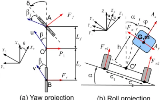
The variables used in the sequel, reported in the Fig.1, are listed below:

• θ is the vehicle yaw angle,

θ δ O' A B u vβr β_f β c₁ O' Fn1 Fn2 Az G,m h

(a) Yaw projection (b) Roll projection

Ff Fr X0 Y0 Y1 X1 Y1 Z2 Z1 Y2  α α Z3 Y3 α φ P1 c₂ Ay Fa Lf Lr

Fig. 1. Yaw/Roll dynamic model.

• α is the bank angle of the terrain in the roll projection, • δ is the steering angle,

• u is the linear velocity at the center of gravity, • Lf and Lr are the front and rear vehicle

half-wheelbases,

• Iz is the yaw moment of inertia,

• P1= mg sin(α) is the influence of the gravity force on

the lateral dynamics,

• c1 and c2 are the vehicle half-track,

• h is the distance between the roll center and the vehicle center of gravity G,

• Ixis the pitch moment of inertia,

• Ay. ~Y3 and Az. ~Z3 are respectively the lateral and the

vertical acceleration. They are measured by an ac-celerometer, which take into account the gravity accel-eration.

• Fn1 and Fn2 are the normal component of the

tire-ground contact forces on the vehicle left and right sides,

• Fa(ϕ) is a restoring-force parametrized by kr and br,

the roll stiffness and damping coefficients:

→ Fa= 1 h(krϕ + brϕ)˙ → y3 (1)

where ϕ is the roll angle of the suspended mass asso-ciated to the roll dynamics, depicted on Fig.1.

The forces Fr and Ff are modelled with a linear model

(2) like in [10]:

Ff = Cf(.)βf

Fr= Cr(.)βr

(2) Although a linear model is used, the non-linearity and the grip condition variations are taking into account, because the cornering stiffnesses are on-line adapted thanks to the observer detailed in section III-B.

B. Yaw mechanical model

In view of the Fig.1, the yaw dynamic can be represented by a state space linear system (3):

¨ θ = a11θ + a˙ 12β + b1δ (3a) ˙ β = −F + mg sin(α) vm − ˙θ (3b) F = Cf.βf+ Cr.βr (3c) with: a11= −(Lf.C2f+L2r.Cr) uIz , a12= (Lr.Cr−Lf.Cf) Iz and b1= Lf.Cf Iz

This model will be used by the observer developed in section III-B.

C. LLT definition

The Lateral Load Transfer (LLT) represents the unbal-anced repartition of the normal components of the tire-ground contact forces. It is mathematically defined as:

LLT = Fn1− Fn2 Fn1+ Fn2

(4) According to the definition (4), the LLT reaches ±1 when two wheels on a vehicle’s side lift off, which is representative of a rollover risk. In practice a threshold is chosen above when the vehicle is considered in a hazardous situation. This threshold is chosen as 80 % (classical value used in the literature) in order to define a safety margin.

D. LLT computation

In previous work [10], the LLT estimation required among several variables the knowledge of two non-measurable vari-ables: the global sideslip angle β and the slope α. They are estimated thanks to an observer. However, if they were incorrectly estimated, the current LLT was also incorrectly evaluated and so the predicted LLT.

To address this problem, the new roll model depicted Fig.1(b) is used. Thanks to the fundamental principle of the dynamic applied to this model, and still assuming that the angles are small, dynamics equations for the roll angle ϕ and for the LLT are respectively given by (5):

˙ ϕ = m.h.Ay br −kr br ϕ Fn1=

(m.Az− Fasin ϕ)(c2− h sin ϕ)

c1+ c2

Fn2=

(m.Az− Fasin ϕ)(c1+ h sin ϕ)

c1+ c2

(5)

This new model depends only of the lateral and verti-cal accelerations. Theses variables can be measured by an accelerometer. So the LLT can be estimated even if the global sideslip angle and the slope have not been estimated. Moreover the addition of an accelerometer sensor stays in line with the limitation of a low cost sensor equipment.

However, if the LLT have to be anticipated, the lateral acceleration has to be predicted. Considering the yaw model, the lateral acceleration is given by (6):

Ay = u ˙β cos(β) + ˙u sin(β) + u ˙θ cos(β)

| {z } Yaw acceleration + g sin(α) | {z } gravity acceleration (6) In view of equations (6), the lateral acceleration is com-puted relying on the global sideslip β and the slope α, variable which are not measured. So an observer system is necessary to estimate them. It is described in the next section.

III. ROLLOVER PREVENTION SYSTEM A. System overview

The system can be summarized by the following diagram (2):

ATV

LLT Estimation/Prediction

UST Observer

Driver

OST Observer

Decision System

Fig. 2. Algorithm overview.

1) ATV box: The ATV is manually controlled , i.e. the driver specifies the vehicle speed v and steering angle δ. As described in the introduction, the measured data are the roll/yaw rate, the accelerations, the speed and the steering angle.

2) Observer System box: This system allows the on-line estimation of the sideslip angle bβ, yaw rate bθ and the bank˙ angle α whatever the vehicle state. Moreover, a cornering stiffness estimation is supplied to take into account the grip condition variations.

3) LLT Estimation/Prediction box: Relying on the mea-sured and observed variables (v, δ, θ, bb˙ β and α), current LLT values can be on-line estimated (see II-D). And thanks to a predictive algorithm (see [10]) based on the rider’s action extrapolation, the LLT is anticipated by the lateral acceleration prediction. If the predicted LLT is upper than the threshold the pilot is warned of the rollover risk. B. Observer principle

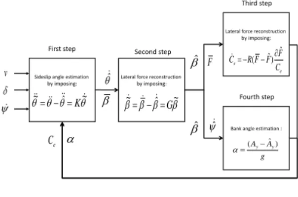
1) Observer model: Like the one developed in [10], This observer is based on the previous yaw mechanical model (see II-B). However for observability reasons, the two cornering stiffnesses cannot be estimated separately, and are therefore considered to be equal to a global virtual cornering stiffness Ce. A backstepping approach has been proposed in [10] and

resumed in the Fig.3.

In the first step, β is calculated to ensure the convergence of θ to ˙b˙ θ: (3a). Then F is calculated to ensure the conver-gence of bβ to β: (3b). Finally, Ceis calculated to ensure the

convergence of bF to F : (3c).

In [10], the slope was estimated by a Kalman filter using the lateral acceleration and the roll rate. Here, the estimation is done within the observer via the addition of a fourth step. This step is detailed in the next section.

2) Roll angle estimation: In view of (6), a model of the measured lateral acceleration has been proposed. As we know now all the variable in (6) excepted the bank angle, α can be estimated using this equation:

α = arcsinAy− u ˙ b

β cos( bβ) + ˙u sin( bβ) + u ˙θ cos( bβ)

g (7)



F

ˆ

Sideslip angle estimation by imposing:    ~  ˆ ~ K    First step    ~ ˆ ~ G      Second step e e C F F F R C( ˆ)ˆ Third step e C ˆ  

v Lateral force reconstruction by imposing:

Lateral force reconstruction by imposing:

Bank angle estimation :

g A Ay ˆy) (    ˆ ˆ Fourth step 

Fig. 3. Observer overview.

C. Observer limitation

Depending of the grip conditions between the front and the rear vehicle (respectively Cf and Cr) and the mass

distribution (mechanical design, driver position, the load...), a vehicle can be under- or over-steering. In view of [12], the vehicle behaviour in the yaw model can be resumed by the following equation (8):

ξ1= Lr.Cr− Lf.Cf (8)

This criterion represents the grip difference between the front and the rear vehicle, whose their importance depends on the gravity center position. So, on one hand, if ξ1 > 0, the

vehicle is under-steering. On the other hand, if ξ1< 0, the

vehicle is over-steering.

In view of the observer equations (3), ξ is present into the coefficient a12. Because of the global cornering stiffness

assumption, the a12 coefficient sign is linked to the center

gravity position (Lf and Lr). So the model is not able to

represent on-line the both behaviour.

With a smooth driving, the vehicle stays under-steering: Cf and Cr are almost equal and Lr > Lf by mechanical

design. However, if the driving has to be aggressive, the mass distribution may change during a bend. It implies a grip condition variation between the front and rear wheels. Moreover, the case with a different floor under the front and the rear wheels is not impossible on off-road context.

In the case where the observer is not representative of the vehicle behaviour, the global sideslip angle β will be miscalculated. This error implies a badly lateral acceleration prediction and so the LLT will be wrongly predicted, espe-cially if β is high.

A solution based on two observers modelling an over- or an under-steering vehicle, has been developed in the next section to take into account this phenomenon.

D. Observer system

1) Dual observer: The “Observer system” box can be represented by the Fig.4. It is composed of two observers and a “supervisor” algorithm.

The UST (Under-STeering) and OST (Over-STeering) observers represent respectively an under- or an over-steering

UST Observer

3 axes Acc.

˙ψ, v , δ

OST Observer

Decision System

observer data

Fig. 4. Algorithm overview.

vehicle. They are similar to the one described on section III-B. As the sign of the a12coefficient defines the vehicle sate,

the value of a12 is defined as following:

UST observer: a12=    (Lr−Lf)Ce Iz   , a12> 0 OST observer: a12= −    (Lr−Lf)Ce Iz   , a12< 0

In the same time, they estimate on-line the dynamical variables (β, Ce, α, ...). Then, the “supervisor” algorithm,

presented in the next section, selects the right observer data to send to the LLT prediction algorithm.

2) “Supervisor” algorithm:

a) Criterion of the vehicle state: Classically, the ex-pressions ((8) and (9)) allows the knowledge of the vehicle state (under- or over-steering). The first has been detailed previously (see III-C) and it is not usable as the front and the rear cornering stiffnesses cannot be differentiated. The second compares the yaw rate without sliding to the actual one ˙θ. It uses the projected linear velocity along the vehicle direction (vx), which requires the knowledge of the global

sideslip angle ( bβ). However as bβ cannot be measured, if its estimation becomes false, the expression (9) would be false too, and the inappropriate observer would be chosen, and so on.

ξ2=

vxtan δ

L − ˙θ (9) As none of these criterions can be used to the estimate the vehicle behaviour, the next section proposed a solution.

b) Proposed solution: If there is a different mechanical behaviour (under/over-steering) between the vehicle and the model, the a12 coefficient will have the wrong sign. As the

β calculation is proportional to a12 , it will have also the

wrong sign. However, the F sign depends principally on the yaw rate ˙θ sign, so even if β has the wrong sign, F will keep the right. But bF will have the opposite sign to F , as bF depends on β. In view of (3) and with a strictly positive Ce,

b

F cannot converge to F , the observation is frozen. So, the more the lateral dynamic is high, the more the lateral force convergence error ( ˜F = F − bF ) will be high too.

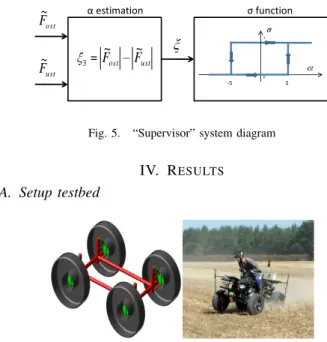
So, the principle is to compare the lateral force conver-gence error between the two observers. The criterion can be defined by (10):

˜

FOST = FOST − bFOST

˜ FU ST = FU ST − bFU ST ξ3=    ˜ FOST   −    ˜ FU ST    (10)

ξ3 is build to be positive or negative, if the vehicle is

respectively under- or over-steering.

c) Observer selection function: If the whole estimated variables of the UST and OST observer are represented by a matrix (respectively XU ST and XOST), the chosen state

can be evaluated by the following function (11): X = σXU ST + (1 − σ)XOST

and with σ = 1, if ξ3> 0, otherwise σ = 0

(11) Moreover a hysteresis function is used to avoid the unde-sirable switch happening when ξ3 is close to 0. This

hys-teresis function is parametrized by S. Its value may change between the simulations and the full-scale experimentations. This algorithm is represented by the diagram Fig.5.

ust ost F F~ ~ 3 ost F~ ust F~ 0 1 α estimation σ function -S S

Fig. 5. “Supervisor” system diagram IV. RESULTS

A. Setup testbed

Fig. 6. MSC Adams ATV and MF400H, Massey Fergusson In order to validate the necessity of a dual observer, if the roll-over situations have to be accurately anticipated, simulation and experimental results are presented. On one side, an ATV has been designed for the simulation with the multibody dynamics and motion analysis software: MSC Adams. On the other hand, experimental results have been performed with a quad bike MF400H, manufactured by Massey Fergusson and depicted in the Fig.6. Its dynamic parameters m, Iz, kr, br, h, Lfand Lrhave been preliminary

calibrated, and it is equipped with the following sensors:

• a Xsens MTI IMU providing accelerations and angular velocities.

• a Doppler radar supplying the linear speed

• an angular sensor providing the steering angle

This set of sensors constitutes a low cost perception system (compared to the ATV cost) enabling LLT estimation without requiring for expensive sensors. In addition, dynamometric sensors supplying tire/ground forces have been set up at each wheel. They provide a ground truth, but are not used in the algorithm.

B. Simulation results

1) ATV simulation path: The simulation aim is to repre-sent a driver who arrives too fast in a curve (8 m s−1). He turns more and more the steering wheel to follow the path until a moment where the vehicle goes over-steering. Then the driver counter-steers to keep the trajectory, but the vehicle spins around at 6.5 s. The grip conditions corresponds to a wet grass flat terrain. The path is presented in the Fig.7.

X [m] Y [ m ] 0 30 10 Vehicle spins round

Fig. 7. Vehicle path 2) Dual Observer:

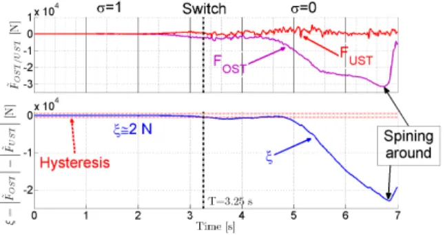
a) ξ3 estimation: The Fig.8 represents on top the

UST/OST lateral force observation errors ( ˜FU ST and ˜FOST),

and the estimation of α: the dynamic behaviour criterion. The hysteresis parameter S is fixed at 500 N, because this value corresponds to an 1.1 m s−2 lateral acceleration with a 450 kg mass. Less than this acceleration, the β observations is possible but the vehicle state differentiation is not possible.

Fig. 8. The divergence of the under-steering observer As the vehicle goes in straight line at beginning, the lateral acceleration is too low to impose a observer divergence. The UST observer is selected by default, because the low lateral dynamic and the mass distribution impose actually an under-steering state.

According to the simulator, the vehicle state is under-steering until 3.35 s. In view of the Fig.8, the “supervisor system” detects the vehicle state switching at the same time 3.25 s.

Finally, the ξ3criterion is able to estimate the vehicle state.

The next section shows the importance of this switch on the β estimation.

b) Global sideslipβ: The Fig.9 represents the different global sideslip β: the under/over-steering observer, the one chosen by the decision system and the one measured by the software. They are respectively plotted in magenta, red, blue and black.

Before the switch, the UST sideslip angle follows the one measured but with a significant overestimation due to the low dynamic (see IV-B.2.a).

Fig. 9. The global sideslip angle β

After the switch, the estimated sideslip angle bβ from the OST observer follows the one measured. On contrast the one from the UST observer has the opposite sign. This sign error influences widely the lateral acceleration prediction and so the LLT prediction too. It is the subject of the next section. C. Experimental results

In order to confirm the influence of the dynamical be-haviour and so the sign of the global sideslip angle on the LLT prediction, full scale experimentations have been done on the quad bike presented in IV-A. One of those is presented in this section.

1) ATV simulation path: This experimentation have been done at an average speed of 5 m s−1 on a mix terrain: wet grass, sloped wet grass and asphalt. The path is represented on the Fig.10. X [m] Y [ m ] 0 60 40 Start _{Curve 4} Curve 3 Curve 1 Curve 2 Asphalt Wet grass 20° slope Sloped wet grass

Fig. 10. Vehicle path

2) LLT estimation: The measured and the estimated LLT are plotted on the Fig.11 respectively in black and blue.

Fig. 11. Measured and estimated LLT

The equation simplification to estimate the LLT compare to [10] does not imply a loss of accuracy. Moreover, the LLT can be estimated even if the observer are not available as the acceleration measures are used (see section II-C).

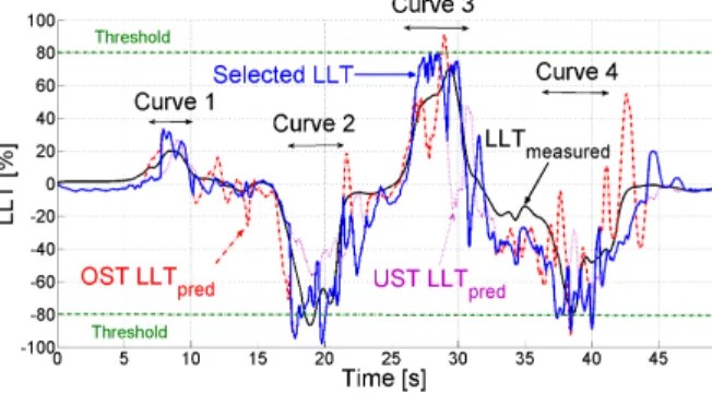
3) Predicted LLT: The Fig.12 represents the different predicted lateral load transfers: with the under- and over steering observer. They are respectively plotted in dashed magenta and dashed-dot red. The LLT predicted with the right observer data recovers the OST or UST predicted LLT and it plotted in solid-blue. The σ variable have been manually set to 1 or 0, respectively to predict the LLT with a single UST or OST observer. Moreover the measured (black) LLT is plotted.

Fig. 12. The different experiment LLT

First, The decision system selects always the right observer during the curve, which is the moment when there is a rollover risk. During the curve 2, the LLT predicted with the OST observer (the one selected) anticipates sufficiently the actual one, whereas the LLT predicted with the UST observer is clearly false. And inversely with the curve 4. For the curve 3, as the driver turns on a low grip condition terrain (wet grass terrain) with an important high speed and/or steering angle, the vehicle behaviour switches during the bend. The decision system selects the right observer. Either the predicted LLT anticipates the actual one during the transitional period, or it follows the actual one. Secondly, the bank angle is correctly estimated, as the selected LLT is accurate during the sloped part.

Finally, sometimes the decision system selects the false observer. Theses mistakes can be observed at 22.5 s and at 31.5 s. The vehicle goes straight line or turns with a low yaw rate, so the both observer are convergent, as explained in IV-B.2.a. Consequently, the ξ3value is around zero and the

decision system is unable to select the good one. However, there is no rollover risk during this situation and the predicted LLT value is not enough high to warn the driver. So theses mistakes are not important since the driver is only warn during the situation with a risk of rollover.

V. CONCLUSIONS AND FUTURE WORKS This paper proposes an algorithm able to anticipate a rollover risk for ATVs motion on natural ground. Two adapted backstepping observers, based on a bicycle model, have been designed in order to estimate the dynamic variables (sideslip angle, cornering stiffness, bank angle ...). They are selected in functions of the vehicle state (under/over-steering). Then, relying on a roll model, the LLT is on-line anticipated using the estimations of the right

observer. The observer is selected thanks to an algorithm which estimates a behaviour criterion.

The main contributions lie in the dual observer and in the new LLT computation. As demonstrated in the experiments, the LLT can be predicted accurately whatever the terrain conditions (grip, bank angle) and the vehicle state. This sensing equipment system is limited to low cost sensors excluding expensive INS, GPS or cameras to be in agreement with a quad bike cost.

Moreover, current developments aim also at developing an active security system able to limit the vehicle speed.

VI. ACKNOWLEDGMENTS

With many thanks to the CCMSA and T. Humbert for respectively the financial and design support.

REFERENCES

[1] “All terrain vehicle enforcement and safety report 2006,” Wisconsin department of natural resources, USA, Tech. Rep., 2007.

[2] CCMSA, “Accidents du travail des salari´es et non salari´es agricoles avec des quads,” Observatoire des risques professionels et du machin-isme agricole, Paris, France, Tech. Rep., 2006.

[3] D. Bevly, J. Ryu, and J. Gerdes, “Integrating INS sensors with GPS measurements for continuous estimation of vehicle sideslip, roll, and tire cornering stiffness,” IEEE Trans. Intell. Transport. Syst., vol. 7, no. 4, pp. 483 –493, 2006.

[4] D. Piyabongkarn, R. Rajamani, J. Grogg, and J. Lew, “Development and experimental evaluation of a slip angle estimator for vehicle stability control,” IEEE Trans. Contr. Syst. Technol., vol. 17, no. 1, pp. 78 –88, 2009.

[5] B. Schofield, T. Hagglund, and A. Rantzer, “Vehicle dynamics control and controller allocation for rollover prevention,” in IEEE Interna-tional Conference on Control Applications, 2006, pp. 149 –154. [6] G. Besseron, C. Grand, F. Ben Amar, and P. Bidaud, “Decoupled

control of the high mobility robot hylos based on a dynamic stability margin,” in IEEE/RSJ International Conference on Intelligent Robots and Systems (IROS), 2008, pp. 2435 –2440.

[7] K. Ohno, V. Chun, T. Yuzawa, E. Takeuchi, S. Tadokoro, T. Yoshida, and E. Koyanagi, “Rollover avoidance using a stability margin for a tracked vehicle with sub-tracks,” in IEEE/RSJ Safety International Workshop on Security Rescue Robotics, 2009, pp. 1 –6.

[8] S. Peters and K. Iagnemma, “An analysis of rollover stability mea-surement for high-speed mobile robots,” in Robotics and Automation, ICRA, May 2006, pp. 3711 –3716.

[9] M. Spenko, Y. Kuroda, S. Dubowsky, and K. Iagnemma, “Hazard avoidance for high-speed mobile robots in rough terrain,” Journal of Field Robotics, vol. 23, no. 5, pp. 311–331, 2006.

[10] M. Richier, R. Lenain, B. Thuilot, and C. Debain, “On-line estimation of a stability metric including grip conditions and slope: Application to rollover prevention for all-terrain vehicles,” in Int. Conf. on Intelligent RObots and Systems (IROS), 2011.

[11] S. Peters, “Stability measurement of high-speed vehicles,” Vehicle System Dynamics, vol. 47, no. 6, pp. 701–720, 2009.

[12] G. Genta, Motor Vehicle Dynamics: Modeling and Simulation. World Scientific, 1997.