Distance sensing via magnetic resonance coupling

D

D

e

e

g

g

r

r

e

e

e

e

C

C

o

o

u

u

r

r

s

s

e

e

S

S

y

y

s

s

t

t

e

e

m

m

s

s

E

E

n

n

g

g

i

i

n

n

e

e

e

e

r

r

i

i

n

n

g

g

M

M

a

a

j

j

o

o

r

r

:

:

P

P

o

o

w

w

e

e

r

r

&

&

C

C

o

o

n

n

t

t

r

r

o

o

l

l

D

D

i

_i

p

_p

l

_l

o

_o

m

_m

a

_a

2

₂

0

₀

1

₁

3

₃

O

O

r

r

l

l

a

a

n

n

d

d

o

o

S

S

u

u

m

m

m

m

e

e

r

r

m

m

a

a

t

t

t

t

e

e

r

r

D

D

i

i

s

s

t

t

a

a

n

n

c

c

e

e

s

s

e

e

n

n

s

s

i

i

n

n

g

g

v

v

i

i

a

a

m

m

a

a

g

g

n

n

e

e

t

t

i

i

c

c

r

r

e

e

s

s

o

o

n

n

a

a

n

n

c

c

e

e

c

c

o

o

u

u

p

p

l

l

i

i

n

n

g

g

Distance sensing via magnetic resonance coupling

Graduate

Bachelor’s Thesis

| 2 0 1 3 |

Power & Control

Supervising professor Joseph Moerschell Expert

Sousuke Nakamura Partner

Hashimoto laboratory, Chuo University, Tokyo

Objectives

The goal is to understand how the principle of distance determination via resonant magnetic coupling based on the researches of Hashimoto laboratory works and to perform measurements.

Methods | Experien ces | Resu lts

Mobile devices or robots can be charged wirelessly using the magnetic resonance coupling. Some types of robots work independently. A position location system is necessary for the robot to know where it is. For this reason the possibility to determine the position based on magnetic resonance coupling is investigated. In this way a system handling two tasks, can be developed in one, i.e. charging the battery and locating the position in a building or in a room.

Attention was focused on the distance sensor. The position cannot be calculated directly but it can be determined via a comparison with a table. The reflection coefficient or the equivalent circuit impedance of the coupled antennas must be measured for this comparison. The necessary calculations for determining the position and the error analysis were made with Matlab. The measurements show that the determination of the distance can be carried out in this manner. However, the range is limited and the area within which the error is small, varies according to the antenna parameters.

Antenna setup used for measurements

Picture

(optional)

300 dpi

6.5 x 5cm

1

TABLE OF CONTENTS

1 TABLE OF CONTENTS ... ... ... 1

2 INTRODUCTION ... ... ... .. 1

3 THE PRINCIPAL FUNCTIONALITY OF THE PROPOSED SENSOR ... ... 2

4 INVESTIGATION, USING THE EQUIVALENT CIRCUIT ... ... ... 3

5 METHOD FOR POSITION ESTIMATION ... ... ... 5

6 CONVERSION OF THE REFLECTION COEFFICIENT IN THE COUPLING COEFFICIENT ... ... 6

7 ESTIMATING THE POSITION BASED ON THE COUPLING COEFFICIENT ... ... 8

7.1 Geometrical relation between the coils ... ... 8

8 BASIC CHARACTERISTICS OF THE DISTANCE SENSOR ... ... ... 12

8.1 Distance estimation method ... ... ... 12

8.2 Relationship between design parameters and model errors ... ... 13

8.3 Relationship between effective range and the design parameters ... ... 15

8.3.1 Behaviour of the coupling coefficient measuring errors in relation with the distance ... ...15

8.3.2 Determination of the minimal error point ... ... 22

8.3.3 Characteristics of the distance error as a function of the distance ... ...27

9 MEASURING OF THE DISTANCE SENSOR ... ... ... 28

9.1 Measurement of the design parameters ... ... 29

9.2 Determine the position based on a database interpolation ... ... 30

9.2.1 Results for a receiver antenna resistance without additional resistance ... ...32

9.2.2 Results for a receiver antenna resistance of R2 46.64 ... ...35

10 ALTERNATIVE MEASUREMENT OF ... ... ... 37

10.1 Simulation ... ... ... ... 37

10.2 Measurement ... ... ... . 38

11 CONCLUSION ... ... ... ... 39

12 DATE & SIGNATURE ... ... ... 39

13 APPENDICES ... ... ... .... 40

14 USED EQUIPMENT ... ... ... 41

DISTANCE SENSING VIA MAGNETIC RESONANCE

COUPLING

2

INTRODUCTION

This work was written as part of a student exchange and was created in collaboration with the Chuo University in Tokyo. I'm worked, in relation to this exchange, in collaboration with the Hashimoto laboratory. The goal is to write a work related to a current topic of this la-boratory. This work is based on the work over position sensing based on magnetic reso-nance coupling from Hashimoto laboratory [1], focusing on the distance sensor.

The idea behind this project is, position sensing and power supply for robots. It is possible to recharge the robot cable less via coils. If it is possible, the position over coils to deter-mine, can be build a system which makes two tasks in one. One possible application is, for example, a factory in which parts via robots from A to B to be transported or robots that act in an intelligent space to facilitate everyday life. The tracking system allows the robot to determine he's position within the factory or the room. If the batteries are discharged, the robot can go to the charging station and recharge himself, with the help of the re-charging system, or it can be used the same coils as are used for the position sensing The first part of the work is to understand how functioning this type of sensor. Therefore, the individual areas were investigated and as possible derive by myself. If possible, have been using Matlab to create functions for the processes to simulate and to understand them better

In the second part of the analysis was focused on the distance sensor and two antennas were produced and measured. The evaluation of the results was performed using Matlab. To improve the knowledge of Matlab was casually reading a book over Matlab [2].

3

THE PRINCIPAL FUNCTIONALITY OF THE PROPOSED

SENSOR

The sensor consists of four transmitters and one receiver. The transmitters and the re-ceiver are coils, and they are coiled from copper wire. The transmitters can be individually switched on and off. For the position detection always only one transmitter is active. That’s the non-active transmitter not influents the result, is a second switch used to cut off some circuit elements. Thereby changes the resonance frequency of the non-activated transmitters. The basic principle is schematically shown in Figure 1.

Figure 1 : Schematic illustration of the basic structure [1]

The magnetic resonance coupling with the receiver is incurred if one of the transmitters will be enabled. The coupling coefficient is used to estimate the position. But this coeffi-cient can’t be measured. For this reason, the reflection coefficoeffi-cient is measured, and from this the coupling coefficient is determined. With one transmitter antenna, only the distance between the transmitter antenna and the receiver antenna can be estimated. That is why, different transmitter antennas for the position estimation in a three dimensional room are used.

The four transmitter antennas are turned-on one after another, in order to measure the corresponding reflection coefficient. The reflection coefficient vector is made on basis of the measured values.

4

INVESTIGATION, USING THE EQUIVALENT CIRCUIT

In the previous section 3 is assumed that always, only one transmitter antenna is turned-on. For this reason, contains the circuit analysis only the coupling between one transmitter antenna and the receiver antenna. For this case the equivalent circuit shown in Figure 2 can be used. Transmitter and receiver antenna consist of different circuit elements. Each antenna containing, connected in series a resistor R , a capacitor and a coil i 1,2 . Thus, each circuit for the antennas corresponds to a resonant circuit. is the power source and supplies the transmitter antenna with energy. Z is the characteristic imped-ance of the transmission line between the power source and the transmitter antenna.

Figure 2 : Equivalent electrical circuit for the magnetic coupling [1]

For reducing the electrical losses, the principle of magnetic resonance coupling is used. The magnetic resonance coupling will be strengthened if both antennas have the same resonance frequency. The resonant frequency for the circuit in Figure 2 is calculated by using the Equation 1 and must be the same for both circuits. The reactance X must be-come equal zero to obtain the resonance frequency.

.

!

"

#

_"

1

!

$"

%

1

$"

0 ' 1,2 ,

"

2()

Equation 1 : Determining the resonant frequency

) is the resonant frequency " is the angular frequency from the resonate frequency. If the circuits are coupled, the equivalent circuit diagram from the right side of Figure 2 can be used. The coupling coefficient * is a dimensionless size and describes the intensity of the magnetic coupling between the antennas. The coupling coefficient is given from Equa-tion 2. ₊ is the mutual inductance and changes with the distance between the antennas. The mutual inductance is the only variable size in this equivalent circuit because she's de-pending from the coupling coefficient. The relation between the coupling coefficient and the mutual inductance, is Described from Equation 2.

*

,

Equation 2 : Coupling coefficient [1]

/0 is the equivalent impedance of the complete circuit for the transmitting and receiving

antenna. /₀ is described as follows.

/

1

%

_$"

1

-

% $"

#

%

$"

21

% 1

_$"

% $"

#

3

$"

% 1

% 1

_$"

% $"

#

Concerning to the relationship from the Equation 1, can this equation be simplified.

/

1

# $"

%

_$"

$"

1

# $"

% 1

# $"

By forming and simplify the final result is obtained in Equation 3.

/

1

%

"

+.

1

5

METHOD FOR POSITION ESTIMATION

With this position estimation procedure, is the reflection coefficient used as the measured value. This value changes to in relation with the distance between the antennas. This is the reason why the coupling coefficient can be determined by using the reflection coeffi-cient. The reflection coefficient can be measured by using a bidirectional coupler as shown in Figure 1.

The reflection coefficient Γ is a Physical quantity that describes the relationship between the voltages of an incident to a Reflected wave. If the reflection coefficient is set to the square is obtained a relationship between the incident and reflected power.

The transmitted power from the transmission antenna can be grouped into two areas. One part of the energy receives the receiver antenna, due to the magnetic resonance coupling. The remaining energy flows through the room, and the receiving antenna without the en-ergy is gathering. This part of the enen-ergy flows back to the transmitting antenna. The rela-tionship between the received and the reflected power can be described with the coupling coefficient

*.

• _{The coupling coefficient}

*

• _{The reflection coefficient} Γ _{is in relation to the coupling coefficient}

*

As described in Section 3 the proposed position sensor has four transmit antennas for de-termining the position of the receive antenna. For this reason, vectors are introduced to describe the data of the four antennas. The reflection coefficient vector is made by meas-uring the reflection coefficients for each antenna pairs (each between a transmitting and the receiving antenna). Thus it can be determined the location of the receiving antenna over the reflection coefficient vector. For this, the measured reflection coefficient vector must be converted in to the coupling coefficient vector.

6

CONVERSION OF THE REFLECTION COEFFICIENT IN

THE COUPLING COEFFICIENT

The relation between the coupling coefficient and the reflection coefficient can be deter-mined by analysis of the circuit from the section 4 and the description of the Q-factor Analysis. First, the Q-factor is described Equation 4.

5

"

₁

!

' 1,2 ,

5 ,5

5

Equation 4 : Determining the Q-factor [1]

The Q-factor is the indicator for the quality of the resonant frequency. The relation be-tween the coupling coefficient and the equivalent circuit impedance /₀ can be described with Equation 3, Equation 2 and Equation 4.

+.

*

By using this relationship to the Equation 3 is obtained the following expression:

/

1

%

"

1

1

%

"

_*

1

By inserting the circuit elements, the Equation 4 can also be written as follows:

5 6

"

₁

-

1

If this last Description is compared with the previous equation, the equation for the equiva-lent circuit impedance Equation 3 is added as follows:

/

*

5

1

% 1

*

5

% 1 1

1

%

"

1

The reflection coefficient is determined from the equivalent circuit impedance

/

/

Γ

/

_/

# /

0

% /

Equation 6 : Determination of the reflection coefficient [1]

The reflection coefficient is translated into the coupling coefficient by using the Equation 5 and the Equation 6. For the calculation are the values for the Q-factor, R_- and Z as fixed values used. Thus, the reflection coefficient vector Γ7 Γ_-, … , Γ₉ which describes the measured values of the reflection coefficient between the antenna pairs can be translated into the coupling coefficient vector *7 *_-, … , *_: , which describes the coupling coeffi-cient between antenna pairs. M corresponds to the number of transmitter antennas.

7

ESTIMATING THE POSITION BASED ON THE COUPLING

COEFFICIENT

In the previous section 6, the coupling coefficient is determined by using the measured re-flection coefficient. In this section is the position determined, from the previous determina-tion of coupling coefficient and his mathematical reladetermina-tion to the mutual inductance. For this the mutual inductance must be determined mathematically. The mutual inductance can be calculated from the Neumann equation, Equation 7. This equation describes the mutual inductance between two circuits _- and _. for one winding ; 1.

+

_{4( = =}

<

>?

_@

>?

AC

Equation 7 : Neumann equation[1]

< is the permeability of the space, >?- and >?. are small line elements of the circuits for

the transmitter and the receiver antenna. @_-. is the distance between the line elements >? -and >?_..

7.1

Geometrical relation between the coils

This section will insert the geometric relationship into the Equation 7. For this, is the Sca-lar product of dl_- and dl_. and the relation of r_-. is analysed. In this case, it is assumed that the transmitter and the receiver antenna are oriented parallel to each other. The ge-ometrical relation is shown in Figure 3. >?_- and >?_. can be written as follows:

| dl-|

>2∗

,

>2∗

The scalar product from >?_- and >?_. can be determined as follows.

>?

>?

|

|

|

|

4 ∗ cos M1# M2 ∗ dθ1 dθ2 Equation 8 : Scalar product of

>?

∗ >?

The distance @_-. is determined by using the orthogonal projection. For the analysis is the displacements projected on the base of the respective axis. Two of the projected distanc-es are in the same plane as the transmitting antenna. The projection for the height differ-ence is vertical to this plane. The projections are expressed in polar coordinates. The dis-tance @_-. can be expressed as follows.

@

_N

_{sin P}

_{% NQRS P #}

>

2 cos M

# cos M

%

>

2 sin M

# sin M

By multiplying out the brackets and grouping the terms we get:

@

N

sin P

% cos P

# 2N cos P

>

_{2 cos M}

# cos M

%

>

4 cos M

%

cos M

% sin M

% sin M

# 2 cos M

cos M

% sin M

sin M

This expression can be more simplified, by using the following relations:

cos T cos U % sin T sin U

cos T # U ,

VW> cos T

_{% sin T}

₁

By use of these relations it can be written as follows:

@

N

% N> cos P cos M

# cos M

%

>

4 2 # 2 cos M

# M

The final result is obtained by using the square root of it, and the expression

>/2

@

>

₄

68 % 16 ZN

_>[

# 8 cos M

# M

# 16

N

_{> cos P cos M}

# cos M

Equation 9 : geometrical relation of

@

If the geometrical relation for the small line elements dl_- and dl_. Equation 8, and the rela-tion for r_-. Equation 9 in to the Equation 7 will be inserted, is the result the mutual induct-ance L_], how it is described at Equation 10.

+

;

_{4( = =}

<

>QRS M

# M

>M

>M

^8 % 16 ZN>[

# ) M

, M

._

Equation 10 : Neumann equation under consideration to the geometrical relation [1] For the Equation 10 is valid:

) M

, M

8QRS M

# M

% 16

N

_{> cos P cosM}

# cosM

The analytical description of the position is based on the complex description of the mutu-al inductance not possible. N is the number of turns from the coil, d is the antenna diame-ter, g is the distance between the antenna centres and P is the elevation angle. It is as-sumed that (x1, y1, z1) and (x2, y2, z2) are the central position for the transmitter antenna and the receiver antenna.

Figure 3 : The geometric relation between the antennas [1]

The distance g between the centre points of the antennas and the elevation angle P, are described from the Equation 11 and the Equation 12.

N , `

# `

% a

# a

% b

# b

P tan

_f

b

# b

-, `

# `

% a

# a

g

Equation 12 : Determining the elevation angle P [1]

To receive a relation between the geometrical position and the coupling coefficient is the Equation 2 used at the Equation 10. The result is shown at the Equation 13

*

;

,

<

4( = =

>QRS M

# M

>M

>M

^8 % 16 ZN>[

# ) M

, M

Equation 13 : Geometric description of the coupling coefficient *

[1]

For the Equation 13 is valid:

) M

, M

8QRS M

# M

% 16

N

_{> cos P cosM}

# cosM

By use of the Equation 11 and Equation 12 into the Equation 13 is obtained a description which gives the coupling coefficient in relation to the coordinates of the coils. Thus, the position can be determined based on the coupling coefficient. This equation can’t be ana-lytically solved based on the double integral. On this reason it is not possible to determi-nate the position analytically.

In addition, the solution set, of possible coordinate points are elements of a circle, which is located in a certain distance to the coil. This relationship is not surprising, since the inten-sity of a magnetic field at a certain distance around the ring coil is also equal for any point element of a circle around the coil. This relation holds as long the propagation of the field is not affected by external disturbances.

8

BASIC CHARACTERISTICS OF THE DISTANCE SENSOR

The basic characteristics of the distance sensor are analysed by using one pair, corre-sponding to one transmitter antenna and one receiver antenna. It is assumed that only one transmitter antenna is activated. For simplicity, the orientation of the antennas to each other is neglected, that means that the antennas are oriented parallel to one another. Further, the antennas are oriented so that they are precisely superposed, corresponding to the case where the elevation angle P _ _. [rad] corresponding to Figure 3. Thus, the movement is only in one axis possible.

8.1

Distance estimation method

The distance g/d is a dimensionless relation between the antennas distance N and the antenna diameter >. This distance is used for the analysis of the sensor characteristic. The distance estimation is made by executing the following two steps.

• _{Transforming the reflection coefficient into the coupling coefficient.} • _{Derivation of position corresponding from the coupling coefficient}

For the displacement in the z-axis is only one transmitter antenna used for that reason are no vectors used and all values are scalar. For the displacement in the z-axis is used only one transmitter antenna, for that reason are no vectors be used and all values are scalar values. The position is derived from a database comparison. The database is created by using the Equation 14.

*

;

,

<

4( = =

>QRS M

# M

>M

>M

^8 % 16 ZN>[

# 8QRS M

# M

Equation 14 : Determination of the coupling coefficients of the superposed antennas [1] For the Equation 14 is valid:

8.2

Relationship between design parameters and model errors

The difference between the determinate values and the real values is called model error. In the second step for the distance estimation, is the position corresponding to the cou-pling coefficient and the Neumann equation derived. Into the Neumann equation is as-sumed that the current has in the whole circuit a similar value. Therefore, the Neumann equation cannot be used if the electrical length comes to big. In this case is the result an error, because the current in the circuit is unequally distributed. Below is a closer look at the electrical length.

The electrical length is a physical value and is defined from Equation 15.

?

(

_{Q );>}

Equation 15 : Determination of electrical length [1]

The equation for the electrical length contains the following design parameters: The fre-quency ), number of turns ; of one coil and the antenna diameter >. The natural constant Q is the speed of light. The relationship between model error and design parameter is shown from Figure 4 to Figure 6.

Figure 4 : Model error in relationship to the frequency ) [1]

The model error rate is expressed in the base of the coupling coefficient. *_j is the theoreti-cal value, and it is theoreti-calculated by using Equation 14. * is the true value which is determined by magnetic field analysis. This analysis is made by CAD analysis software for electrical components. Thus, the error rate is described as follows:

Figure 5 : Model error in relationship to the number of turns ;, for two different frequen-cies ) [1]

From Figure 4 to Figure 6 show that’s the model error comes smaller if the individual de-sign parameters come smaller. From Equation 15 it’s shown that these three parameters form a product for the determination of the electrical length. Thus, it shows that the error increases if the electrical length comes bigger. The error can be limited by limitation of the electrical length.

.

Figure 6 : Model error in relationship to antenna diameter >, for two different frequencies ) [1]

8.3

Relationship between effective range and the design parameters

An important relation for a distance sensor is the relation between the design parameters and the effective range. The effective range according to an area in that’s the distance er-ror is small. Below, the effective range and the distance erer-ror are investigated as a func-tion of design parameters. The distance error is dependent of measurement error and model error. Following is assumed that the model error is eliminated by reason of limiting the electrical length. Thus, the distance error is based on the measurement error. The measurement error is the variation from the measuring instrument.

The variation from the reflection coefficient ΔΓ is being caused from measuring error. The measurement error is given from Equation 16. The measurement error is given from the datasheet of the used measuring instrument [3]. For the measurement, a bi-directional coupler of an Agilent Technologies E-5061A network analyser was used.

ΔΓ a|Γ| % o

Equation 16 : Determination of the measurement error for the reflection coefficient [1] This error characteristic describes the worst case. For this reason, the real values should be below these values. The error characteristic is approximated as a straight with the slope a = 0.0178 and Intercept b = 0.004.

8.3.1

Behaviour of the coupling coefficient measuring errors in relation with the

distance

An analytical analysis is not possible because the Equation 14 contains a double integra-tion. In this case are the antennas superposed and the elevation angle is φ q _. rad . Thus, the coupling coefficient can be approximate Equation 17. This approximation per-mits a part analytical analysis. Equation 14 can with be simplified with Equation 17.

* r l

_{T v 0}

Equation 17 : approximate determination of the coupling coefficient [1]

With Equation 17 it is possible to describe the coupling coefficient error in relation to the distance. For this, first is determined the absolute error:

In the second step is determined the relative error:

∆*

* r

yT> l

sZtu[

_y

l

∆N T v 0

The expression e{ |/} comes never negative. The coupling coefficient has always a value between 1 and 0. The antenna diameter > is also always positive. Only the damping tor T is a negative value, and stay as absolute value. From this, following the result shown in Equation 18.

∆*

* r |T|

∆N

> T v 0

Equation 18 : Approximated relationship between the coupling coefficient errors and the distance error [1]

From Equation 18 is shown that the coupling coefficient error is proportional to the dis-tance error. For this reason, below the disdis-tance error is replaced by the coupling coeffi-cient error.

First, the error rate of the coupling coefficient will be determined. The error rate of the coupling coefficient is determined from Equation 5, Equation 6 and Equation 16. By using the Equation 5 and the Equation 6 can the coupling coefficient be defined as written in Equation 19.

*

_{5 6}

1

_~

1

-1 % Γ

1 # Γ # 1

Equation 19 : Coupling coefficient based on the determination of the reflection coefficient For the determination of the relative error from the coupling coefficient in relation to the re-flection coefficient, must the Equation 19 to the rere-flection coefficient be derived. The result of the derivation must be divided to Equation 19 and multiplied by the error of the reflec-tion coefficient.

∆*

*

1

*

x*

xΓ

∆Γ

€€15

1

2^ 1

_~

-1 % Γ

1 # Γ # 1

1

~

-1 # Γ % -1 % Γ

1 # Γ

€€

1

5 ^

~

1

-1 % Γ

1 # Γ # 1

∗ ∆Γ

The amount can be omitted, as the result of potency, and a root is always positive or it must be positive. This allows a simplification.

∆*

*

_{Z 1}

∆Γ

~

-1 % Γ

1 # Γ # 1[ ~

1 # Γ

∆Γ

• 1 # ~

% Γ 1 % ~

‚ 1 # Γ

The final result is shown in Equation 20. * is the real value, *̂ is the calculated value from the reflection coefficient. ∆* is the absolute value and is defined as the difference between * and *̂.

∆*

*

1

*

x*

xΓ

∆Γ

a|Γ| % o

~

% 1 Γ # ~

# 1

~

% 1 1 # Γ

Equation 20 : error rate of the coupling coefficient [1] For the Equation 20 is valid:

~

# 1

~

% 1 v Γ v 1, a 0.0178, b 0.004, ~

-1

-/

The error curve from Equation 20 can be calculated and displayed with Matlab. In the first effort is the coupling coefficient calculated from Equation 17. The calculated coupling co-efficient will converted into the reflexion coco-efficient. For this conversion are the Equation 4, Equation 5 and the Equation 6 used. After this, the calculated reflection coefficient is used in Equation 20. In the different plots is always changed one of the following design pa-rameters:

• _{The frequency}

)

• _{The resistance of the transmitter antenna}

1

1

/

This result is not detailed enough because the error in the edge cannot accurate be calcu-lated with the result from Equation 17. One example is shown at Figure 7

Figure 7 : Error curve based on the coupling coefficient of the Equation 17 for following model parameters: / 50 Ω , ; 4, ) 10 kˆb , > 0.075 , 1_- 1 Ω , T #3 For this analysis the curve has always the same form. Only the position of the curve change. The exact value for the damping factor T is also unknown and it must rough be estimated. The opening of the curve changes as a function of T.

Because the assessment from Equation 17 is not detailed enough, this equation is re-placed to the Neumann equation, shown at Equation 14. The rest of the analysis rests same. The calculated coupling coefficient is converted into the reflection coefficient and this is used at Equation 20. The error rate of the coupling coefficient in relation to the dis-tance is shown from Figure 8 to Figure 13. At these plots is always only one design pa-rameter changed.

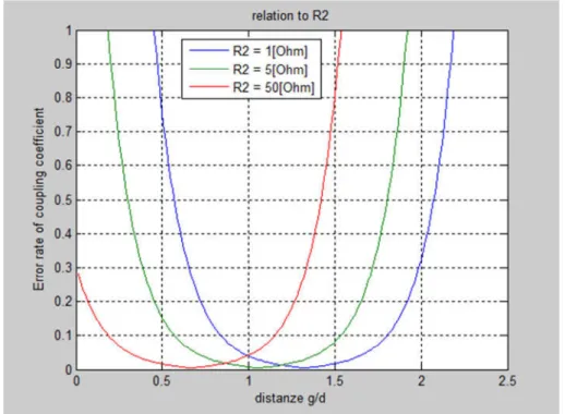
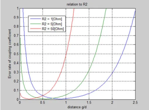
Figure 8 : Error curve for different values of 1_. and the following model parameters: / 50 Ω , ; 4, ) 10 kˆb , > 0.075 , 1- 1 Ω

The error characteristic is independent of the Q-factor. However, the position of the error curve changes in relation to the Q-factor and thus the area of the effective range.

Figure 9 : Error curve for different values of ) and the following model parameters: / 50 Ω , ; 1, > 0.075 , 1- 1. 1 Ω ,

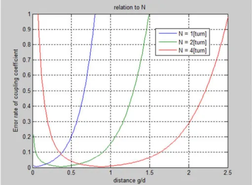
Figure 10 : Error curve for different values of ; and the following model parameters: / 50 Ω , ) 10 kˆb , > 0.075 , 1- 1. 1 Ω

Figure 11 : Error curve for different values of > and the following model parameters: / 50 Ω , ; 1, ) 10 kˆb , 1- 1. 1 Ω

The Figure 8 to Figure 13 was made by using the Matlab Funktion error_Plot t appendix 4. This function requires 6 under functions appendix 5 to appendix 10.

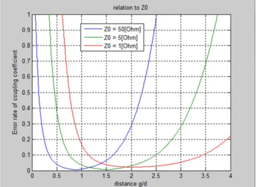
Figure 12 : Error curve for different values of / and the following model parameters: ) 10 kˆb , ; 4, > 0.075 , 1- 1. 1 Ω

Figure 13 : Error curve for different values of 1_- and the following model parameters: ) 10 kˆb , ; 4, > 0.075 , 1. 1 Ω

The error curve is from beginning convex downward up to an effective range. The error curve increase exponentially with increasing distance after overcrossing of this effective range. This behaviour is described in Equation 20. It’s shown that the error comes bigger

8.3.2

Determination of the minimal error point

The error curve must be exactly analysed, In order to find a suitable operating point. The equation from the error curve has two poles, Equation 20. The curve is only defined, for all values they are between these poles. The behaviour in the peripheral regions of the poles can be determined with the limit consideration

?'

∆*

*

i ~

# 1

~

% 1 % o

0

∞

Equation 21 : Limit consideration of the lower limit

The reflection coefficient is in Equation 20 so defined that it aspiring from the positive side to the lower limit. As follows is observed the upper limit.

?'

∆*

_*

i % o

₀

∞

Equation 22 : Limit consideration of the upper limit

Thus, it’s shown from Equation 21 and Equation 22 that’s the error in the peripheral re-gions aspiring against undefined. This behaviour is also shown from the Figure 8 to Figure 13.

To find out in which region the minimum error point located is, must the Equation 20 be derived to the reflection coefficient. Since the reflection coefficient is in the amount, must the Equation 20 derived for 2 areas. From Figure 14 is shown that the reflection coefficient is a value between 1 and -1. The values for a und b are supposed as fix. For other values of a and b change the area of validity from ~_-.

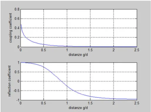
Figure 14 : Change of the reflection coefficient and the coupling coefficient as a function of the distance. This graph was created using the Matlab function K_T annex 11 To simplify the derivation, the denominator from Equation 20 will be multiplied out.

∆*

*

#Γ

_~

_{% 1 % 2Γ~}

a|Γ| % o

_{% 1 # ~}

-Equation 23 : out multiplied formula for the error rate of the reflection coefficient The area of validity is still given by:

~

# 1

~

% 1 v Γ v 1, a 0.0178, b 0.004, ~

-1

-/

To obtaining the minimum value of the curve, must the derivation be equal zero. As first, the area which the reflection coefficient is ≥ 0 will be analysed. As result of the derivation is obtained a quadratic equation. This equation has only one defined zero point and this is defined as follows:

Γ

#

_{i %}

o

‘2o

_{i 3}

%

~

# 1 % 2 oi~

_~

--

% 1

Equation 24 : Minimum error in the positive range of the reflection coefficient One zero point is not in the defined area, for this reason the only defined zero can be de-scribed as shown from Equation 24. ~_- is the only variable coefficient in this equation. Γ_• can’t be negative. Because this, must be locate a valid area for ~_-.

~

’

1

1 % 2 oi

r 0.690

At this point the validity range of basic equation may not be forgotten:

~

# 1

~

% 1 v Γ v 1 #0,183 v Γ v 1,

0 ” Γ

v 1

Thus, all values of the Equation 24 are defined for ~_-’ 0.69.

Following is the area with a negative reflection coefficient inspected. For this, the Equation 23 must be derived for a negative reflection coefficient. Even in this case is the result a quadratic equation. For this equation is only one zero point defined for a negative reflec-tion coefficient. This zero point is defined at the Equareflec-tion 25.

Γ

o

_{i #}

‘2o

_{i 3}

#

# ~

# 1 % 2 oi~

_~

--

% 1

Equation 25 : Minimal error in the negative range of the reflection coefficient

~- is the only variable coefficient in this equation. Γ• can’t be positive. For this reason, a

range of validity for ~_- must be defined.

~

’

1

Also in this case the validity range from the Equation 23 must be compared with this va-lidity range.

~

# 1

~

% 1 v Γ v 1 0,289 v Γ v 1 – #1 v Γ

v 0

It is shown that’s no one of the values from the Equation 25 are defined.

Finally, remains the question how the error behaves in the range of 0.690 — ~_-’ 0. Since this area is not defined for an analytical consideration. The behaviour must be investigat-ed from a simulation. The behaviour was analysinvestigat-ed by using Matlab. The simulations shown that the minimum point of the reflection coefficient is approximate at the zero crossing as long the following values are valid 0.690 — ~_-’ 0. Thus, the minimum point of error based on the value ~_- is defined as follows:

Γ

˜0,

_Γ

_{, ~}

_{’ 0.690}

~

’ 0

Equation 26 : Determination of the reflection coefficient which the smallest error caused. The error curve in relation to the reflection coefficient it is calculated with Matlab. For the calculation is the Equation 20 be used. With the same parameters is the minimum error point Γ_™ calculated by using the Equation 24. The error rate in this point is obtained by in-serting Γ_™ into Equation 20. To verify the Equation 24, the obtained point is printed in the same chart as the error curve. The result is shown at the Figure 15. Since the discovered point actually is located at the minimum point of the curve, the Equation 24 can be re-garded as correct. The graph of Figure 15 was created by using the Matlab function

Figure 15 : blue ~_- 0.01, red ~_- 0.9, green ~_- 1.5

From Equation 19, the coupling coefficient can be determined by using the reflection coef-ficient. This relation can be used at the Equation 26 to determinate, for which value of the coupling coefficient the smallest error exist.

*_+!•

š

›

œ

›

•1

5 6

~

1

# 1,

~

’ 0

1

5 6

~

1

-1 % Γ

1 # Γ

# 1, ~

’ 0.690

Equation 27 : determining the value of the coupling coefficient which have the smallest er-ror

The coupling coefficient comes with higher distance exponentially lower. Based on this, it’s shown from the Equation 27 that the distance for the minimum error comes bigger if the Q-factor of the sensor increases. The Q-Factor is described from Equation 4. This equation contains also the resistance of the transmitter antenna R_-. This model Parameter is also contained at γ_-. Because γ_- influence the error characteristic, it cannot be said that the Q-factor is an independent value. The inductivity of the transmitter and the receiver antenna is given based on their geometrical dimensions. Thus, it rest only the values of f, N, d and 1_. to increase the value of the Q-factor. The values f, N and d are in relation with the model error and this values are limited based on the model error analysis and

limitation of the electrical length chapter 8.2. At the Equation 27 the Q-factor can also be written with the model parameters, this is shown in the Equation 28 and Equation 29. Suppose the transmit antenna resistance R_- correspond to the copper resistance of the coil. In this case, it can be assumed that R_- r 1 and the line impedance corre-sponding Z r 50 Ω , then applies γ_- r 0.02 v 0.69. The value for the minimum error of the coupling coefficient is in this case defined as shown from Equation 28.

*_+!•

_{5 6}

1

_~

1

# 1 6

/ # 1

-"

∗

1

"

,

~

’ 0

Equation 28 : Minimal error of the coupling coefficient

For values of

~

’ 0.690

*_+!•

_{5 6}

1

_~

1

-1 % Γ

1 # Γ

# 1 6

1

"

f/

1 % Γ

1 # Γ

# 1

g ,

~

’ 0.690

Equation 29 : Minimal error of the coupling coefficient

From the Equation 28 und Equation 29 is shown that the effective range decrease if the receiver antenna resistance R_. increase. This behaviour is confirmed from the Figure 8.

8.3.3

Characteristics of the distance error as a function of the distance

The theoretical consideration of the coupling coefficient error is also valid for the distance error. Because the error rate of the coupling coefficient is proportional to the distance er-ror. This relation is shown at the Equation 18. To simplify the end of the analysis, Z and R- are not included in the consideration. There are the following relations.

• _{The distance error is convex decreasing with distance up to a turning point. From} this point the error increases again convex. This means that the error is in the near field as well as in the far field bigger.

• _{If Q is increased, increases also the distance between the transmitting and the} re-ceiving antenna for which is obtained the smallest distance errors.

• _{The distance error is bigger in the near field and smaller in the far field if the} Q-factor is enlarged.

Finally it can be said, that the model parameter must be chooses based on the needed distance. Because the error curve show different areas for the effective range and the minimum error if the design parameters changes.

9

MEASURING OF THE DISTANCE SENSOR

For this measuring were produced two antennas. The measuring contains the equivalent impedance of the two coupled antennas /₀ and the distance between the centre points of the antennas N. The result is a table which contains different values of the impedance /₀ in relation with the distance. The transmitter antenna is supplied over an Agilent Technol-ogies E-5061A Network analyser with a signal frequency of 10 [MHz], the receiver anten-na is passive. The Network aanten-nalyser shows the Smith-chart of the two coupled antenanten-nas. The equivalent impedance /₀ can be read from the display.

The transmitting antenna and the receiving antenna are threaded between two sticks. On one of the two sticks is a scale with a pitch of a 0.5 [cm] recorded. The centre of the transmitting antenna is fixed at zero, and the receiving antenna is moved in steps of 0.5 [cm]. The measurement setup is shown in Figure 16

Figure 16 : measurement setup for the distance measuring

To keep the influence of foreign objects as small as possible, the sticks were placed be-tween two chairs so that the coils are in the air. Important for an accurate calculation of the position is the precise as possible determination of the design parameters.

9.1

Measurement of the design parameters

The design parameters of the antennas must be measured. The inductivity can over a LC circuit and a known value of the capacity been determined. In this case is a capacity of 1 [nF] used. From this circuit must be measured the resonance frequency, and over the resonance frequency can be calculated the impedance for each antenna. The resonance frequency can be determined over a Smith-chart or a Bode-diagram. In this case was used the Smith-chart. This Smith-chart is made from an Agilent Technologies E-5061A Network analyser. For both antennas was the resonance frequency, for the capacity from above 2.9 [MHz]. Thus, the resonance frequency can be calculated from Equation 30.

1

∗ 2()

Equation 30 : Calculation of the inductance based on the resonance frequency and a known capacitance.

From the calculated inductivity can be determined the needed capacity, for which is ob-tained the desired resonance frequency. In this case have the capacity a value in the or-der of 84 [pF]. The resonance frequency is defined from the Equation 31.

)

1

2(√

Equation 31 : Determining the resonant frequency

The fine tuning is made with adjustable capacities. Based on this can the desired reso-nance frequency quite exactly been adjusted. As reference is used a Smith-chart, which is made from an Agilent Technologies E-5061A Network analyser. The marker must be set on the desired resonance frequency. The imaginary part of the antenna impedance must be zero and the real part is corresponding to the antenna resistance R_- or R_.. The receiv-er antenna resistance R_. can be increased via additional resistances. If the receiver an-tenna resistance R_. increase, the Q-factor decreases. This is used to make measure-ments with different Q-factors. For this reason, the receiver antenna resistance is not set as fix. All other model parameters are shown in the Table 1.

Model Parameter

Designation Value Unit Resonance frequency

)

/

1

9.2

Determine the position based on a database interpolation

Since the position cannot be determined analytically another method must be found to de-termine the position. Therefore, the position determination is based on a database interpo-lation shown in this section.

First is made a database. This database is made from a function which is programmed with Matlab. The function name is range this function is shown into appendix 13. the de-sign parameters from the antennas must be written into the quell code. If the function is executed, they draw a plot which shows the error rate of the coupling coefficient in relation which the distance. This plot based on the chapter 8.3.1. In this chapter is shown that the coupling coefficient error rate is proportional to the distance error. The chart provides in-formation about the area in which the error is not too large to find a suitable measuring range.

The main purpose of this function is to write a table. This table is used for the interpolation of the position. This table looks as shown from Table 2.

¢£ distance coupling coefficient Reflection coefficient error % Q-Factor - - - - - - Table 2 : Example of the table for the position estimation

The first line contains only the Q-factor. The Q-factor is only one time be calculated and change not in relation with the distance. From the second line is written the values for the equivalent impedance /₀, the distance N, the coupling coefficient *, the reflection coeffi-cient Γ and the error rate of the coupling coefficient in per cent. This function contains also a filter function. With this filter is possible to choose only the values which are under a cer-tain error in per cent, for example only values which have an error under 10%.

The position estimation in self is made from the function distance_calc appendix 14. This function needs two tables. The first table contains the measured values for the equivalent impedance /₀ and the distance N. The second table contains the values from the first two columns of the Table 2, the calculated values for the equivalent impedance /₀ and the dis-tance N. From this two tables estimate this function the position based on an interpolation. The formula for the interpolation is shown into the Equation 32

'

_/

/

_V¤ # /

0

_V¤ # /

_>R¥W, N¦ ' ∗ N_>R¥W % 1 # ' N_V¤

Equation 32 : Formula for the interpolation

The values for Z_§_up and Z_§_down are taken from the table for the calculated values, and correspond to the next higher and lower value compared with the measured value of /₀. N_V¤ is the calculated distance for the Z§_up and N_>R¥W the distance for Z§_down. The

by this method found distances are compared with the measured distances. The function

distance_calc gives out a table which contains the measured and the estimated distances.

The function plots a graphic which compares the estimated values with the measured val-ues. The plots from Figure 18 and the Figure 21 are made from this function. This function needs also a general offset value.

9.2.1

Results for a receiver antenna resistance without additional resistance

The measured receiver antenna resistance is 1_. 1.26 . The theoretical effective range is shown into Figure 17. Based on this graphic is choose a measurement range from 3 [cm] to 18 [cm].

Figure 17 : Error rate in conjunction with the coupling coefficient for 1_. 1.26

The calculated value is compared with the ideal value. This comparison is shown at Fig-ure 18. Into the FigFig-ure 18 are the calculated values displaced with an offset of 4 [mm]. This offset is for a smaller receiver antenna resistance 1_. bigger. The resistance is with a value of 1.26 [Ohm] relatively small. The curve is displaced already for small changes of 1_. relatively fast. For higher values of 1_. is a measurement error of this value less im-portant.

Figure 18 : Comparison of Calculated with Measured distances

The table with the results is into the appendix 1. After using the offset is the error in a range from 4.5 [cm] to 17.5 [cm] except of a few exceptions under 1%. These exceptions are related to reading errors or inaccurate positioning of the antennas. The measurements confirm that, the error at the edge of the range greater is.

On another day is determined the maximal measurable distance. The measured receiver antenna resistance is 1_. 1.56 . The experimental setup was designed for a great-er distance. For this reason is the orientation less exact as for the previous measurement and thus the precision comes less exactly. The measurement steps are also higher for this measurement is a measuring step of 1 [cm] used.

Figure 19 : Determination of the maximum measurable distance

The table with the results is into the appendix 2. The poorer accuracy of the measurement is not disturbing in this case, because it’s wanted to determine the maximum measurable distance. From the figure 19 can be seen that the maximum distance is at 30 [cm]. For greater distances, the calculated value remains at 30 [cm].

9.2.2

Results for a receiver antenna resistance of

-®.®- ¯°±

The theoretical effective range is shown into Figure 20. Based on this graphic is choose a measurement range from 2 [cm] to 13 [cm]. The upper section was little increased for a better checking of the error behaviour in the border area.

Figure 20 : Error rate in conjunction with the coupling coefficient for 1_. 46.64

The calculated value is again compared with the ideal value. This comparison is shown at Figure 21. Into the Figure 21 are the calculated values displaced with an offset of 3 [mm].

Figure 21 : Comparison of Calculated with Measured distances

The table with the results is in the appendix 3.After using the offset is the error in a range from 3.5 [cm] to 7.5 [cm] except of a two exceptions under 1%. These exceptions are re-lated to reading errors or inaccurate positioning of the antennas. The measurements con-firm that, the error at the edge of the range greater is. Especially in the upper region of the measurement is the error larger. The error behaviour in the lower area could not be de-termined closer since 2 [cm] is the lowest measurable distance due to the geometrical di-mensions of the antennas.

10

ALTERNATIVE MEASUREMENT OF

This section shows a way for measuring the equivalent impedance /₀ without using a network analyser. This is important for building a sensor, which can independent operate. One possibility is, measuring the tension and the current at the entrance of the transmitter antenna. In this case, the measuring point is in front of the transmitter resistance 1 -shown from Figure 2.

10.1 Simulation

For the verification of the possibility to determine the impedance Ze over the tension and the current is made a simulation with Ltspice 4. The circuit as shown from Figure 2 is used. The mutual inductivity ₊ is defined from Equation 2. The coupling coefficient is cal-culated via the function range appendix 13. The model parameters are the same as those used in the section 9. The resistance from the receiver antenna 1_. is 46.64 [Ohm]. The simulation is shown into Figure 22.

Figure 22 : Simulation to determine /₀

For the calculation of the coupling coefficient was used a distance of 3 [cm]. The meas-ured RMS value for the tension was 3.43 [V] and the RMS value for the current was 70.18 [mA]. For this values has the amplitude for the impedance Z_§ a value of 48.86 [Ohm]. From the table for the interpolation has Z_§ a value of 48.23 [Ohm].

10.2 Measurement

Unfortunately it was not possible to measure the current because no suitable measuring instrument was available and the time was not sufficient to get a suitable instrument. The voltage was measured with a Tektronix TDS 2004C oscilloscope. For this reason, it can-not be said that this method also works in reality

11

CONCLUSION

The measurements have shown that is possible to build a distance sensor, which based on two antennas. Given the manufacturing tolerances of the antennas and the possible reading errors, the sensor have after adding a general offset a good accuracy.

Since the position is calculated the measurements confirm the accuracy of the formulas. The error behaviour in the peripheral regions could also be confirmed. This proves that the error analysis is also correct.

It has been shown, that’s the equivalent impedance of the antenna Z_§ can be theoretically determined based on a voltage and current measurement at the entrance of the transmit-ter antenna. This could not be confirmed in practice, due to time constraints.

To understand how the sensor works has took a lot of time. For this reason, the time was not enough to perform additional measurements, and to measure the position sensor too. For the calculation of the position it is important to know the resistance of the receiving an-tenna 1_. as accurately as possible, since the calculation is no longer correct even for small deviations. This consists for some setups of to the copper resistance of the coil. In the case of energy transmission changes the temperature of the coils and with this the value of the receiver antenna resistance 1₂.

The effective range of this sensor can be changed. However, it must be said that the pre-cision at short distances came less exactly if the sensor is configured for higher distances The coupling coefficient decreases exponentially. If it come too small, the measurement is less exactly or impossible. Therefore, it is difficult to produce a sensor for greater distanc-es.

These three characteristics, it is important to get under control to use this sensor success-fully. For properties where accuracy does not play a major role is the effective range the total measurable area. For example, it is for a robot in a building not important to know his position of the mm exact.

12

DATE & SIGNATURE

13

APPENDICES

♦ _{Appendix 1: Measuring 1, small receiving antennas resistance}

1

♦ _{Appendix 2: Measuring 2, small receiving antennas resistance}

1

♦ _{Appendix 3: Measuring 3, big receiving antennas resistance}

1

♦ _{Appendix 5: Code of the Matlab function change_d} ♦ _{Appendix 6: Code of the Matlab function change_f} ♦ _{Appendix 7: Code of the Matlab function change_N} ♦ _{Appendix 8: Code of the Matlab function change_R1} ♦ _{Appendix 9: Code of the Matlab function change_R2} ♦ _{Appendix 10: Code of the Matlab function change_Z0} ♦ _{Appendix 11: Code of the Matlab function K_T}

♦ _{Appendix 12: Code of the Matlab function Error_XaxisT} ♦ _{Appendix 13: Code of the Matlab function range}

14

USED EQUIPMENT

Agilent Technologies E-5061A Netzwerkanalysator Tektronix TDS 2004C Oszilloskop

15

REFERENCES

[1] N. Sosuke, Design Evaluation of Position Sensor based on Magnetic Resonance

Coupling, Tokyo, Japan: Hashimoto laboratory, Chuo university, 2011.

[2] O. Beucher, MATLAB und Simulink Eine kursorientierte Einführung, mitp, 2013. [3] Agilent Technology, ENA-L RF Network Analyzer E5061A and E062A Data Sheet.