Topological modifications of animated surfaces

(1)

HAL Id: inria-00598389

https://hal.inria.fr/inria-00598389

Submitted on 6 Jun 2011

HAL is a multi-disciplinary open access

archive for the deposit and dissemination of sci-entific research documents, whether they are pub-lished or not. The documents may come from teaching and research institutions in France or

L’archive ouverte pluridisciplinaire HAL, est destinée au dépôt et à la diffusion de documents scientifiques de niveau recherche, publiés ou non, émanant des établissements d’enseignement et de recherche français ou étrangers, des laboratoires

Topological modifications of animated surfaces

Damien Rumiano

To cite this version:

Damien Rumiano. Topological modifications of animated surfaces. Graphics [cs.GR]. 2007. �inria-00598389�

(2)

EVASION Team Damien RUMIANO

INRIA Rhˆone-Alpes Second year training period ENSIMAG

ZIRST from june 18th 2007 to august 26th 2007

655 avenue de l’Europe Montbonnot

38334 Saint Ismier Cedex FRANCE

Training period report

Topological modifications of animated surfaces

supervised by Antoine BOUTHORS, Franck HETROY, Matthieu NESME

(3)

List of Figures

1 2D implicit function with level sets . . . 5 2 differents steps of an animated object: the texture has the same deformation as the object 6 3 three surfaces with different topology . . . 6 4 an animated surface is splitting in two components . . . 7 5 Classification of critical points based on the sign of the 3 eigenvalues of the Hessian H(x) 7 6 Ray-traced metaballs rendered with POVRay . . . 8 7 (a)left Marching cubes algorithm (b)right Particule-based sampling . . . 9 8 (a)left initial marching cubes algorithm (b)middle mechanical mesh (c)right geometric

mesh . . . 10 9 (left) initially, there are 3 critical points: 2 maxima and a 2-saddle (middle-right) the

2 maxima disappear and the 2-saddle “becomes” a maximum . . . 12 10 minima vertices (white) and their corresponding regions . . . 13 11 third Bezier interpolation of a discrete scalar field: (left) wireframe (right) shaded . . 15 12 (a)destroy-create (b)detach-connect (c) pierce-spackle (d) burst-bubble . . . 16 13 two components are splitting : perlin noise shader applied . . . 17

(5)

Training Period context

My training period took place in the EVASION team of LJK Laboratory, in the INRIA Rhône-Alpes building. INRIA Rhône-Alpes is the French National Institute for Research in Computer Science and Control, and is located in Montbonnot, near Grenoble (France). Created in december 1992, INRIA Rhône-Alpes research unit is one of the six INRIA research units. It carries out its activities in tight collaboration with public and private laboratories, both national and international. These activities are organized around five research themes: 1. Communicating systems 2. Cognitive systems 3. Symbolic systems 4. Numerical systems 5. Biological systems

The EVASION team — Virtual environments for animation and image synthesis of natural objects — was created on January 1st, 2003. It gathers faculties, PhD students and engineers. The research work of EVASION is dedicated to the modeling, animation and visualization of natural objects and phenomena. EVASION develops fundamental tools for complex natural scene and object specification, for the design of alternate shape, movement and appearance representations, and for the design of algorithms based on adaptive levels of detail to manage complexity optimally. Naturally, the team intends to validate these tools on specific natural scenes ranging from the mineral kingdom (ocean, streams, lava, avalanches, clouds), to the animal kingdom (organ simulation, character face, body and hair, animal movements), without forgetting vegetal scenes (plant morphogenesis, prairies, trees).

Antoine Bouthors, a Ph.D. student at EVASION, proposed me a work on implicit surface triangulation: in fact, it comes after a paper untitled Twinned Meshes for Dynamic Tri-angulation of Implicit Surfaces written by Antoine Bouthors and Matthieu Nesme, and submitted to Graphics Interface on may 2007. My work consisted in the generalisation of the method presented in this paper, because it has some limitations.

In my opinion, a training period in a research laboratory was a real opportunity to use my theoretical knowledges on computer science, but also to discover “the world of re-search”. Furthemore, this work was a good introduction to Images and virtual reality, a specialization provided by the ENSIMAG for third year students.

(6)

Introduction

To better understand the purposes of this work, I will first introduce the mathematical notions I used during this internship, as well as the applications that this work could have in the future.

This work is mainly based on the Morse Theory and on the algorithms presented in [3] and [5], that is why I will give some details about my implementation and its integration in the original program. It is the starting point for the research step because it highlights the main problems of the previous solutions: thus, I will expose the ideas which have been proposed, implemented and tested.

(7)

1 Implicit surfaces and Topology

1.1 Skeleton-based implicit surfaces and surface tracking

Implicit surfaces are a classical way to represent objects in computer graphics. An implicit surface is defined as the set of points that satisfy : F (x) = c where F : R3

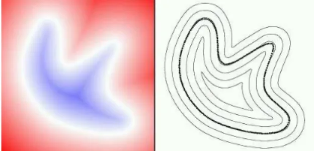
→ R and c is a constant. Figure 1 represents a 2D implicit function with some level sets.

Figure 1: 2D implicit function with level sets

They are a powerful tool for modeling and animating deformable objects such as organic structures or fluids.

Most of the implicit surfaces are skeleton-based. A skeleton is a set of geometric elements such as points and lines that the user can move. To each element is associated an implicit primitive fi: R3 → R which has an influence on the neigbour of the element. And

F(x) =

n

X

i=1

fi(x)

where n is the number of geometric elements.

Hence, by moving one of the elements, the user has a local control on the shape of the implicit surface.

Many implicit primitives are used such as blobby molecules based on the exponential func-tion, metaballs based on polynoms, and soft objects based on the first few terms in a series expansion of a truncated exponential: the exact expressions are given in [12].

Among all these implicit primitives, two have been implemented in the program: • ”pseudo” metaballs (used in [9]):

fi(x) = ( (1 − kpi−xk2 R2 i )3 if kpi− xk ≤ Ri 0 otherwise

where Ri is the radius and pi is the center’s location of the metaball

• cauchy:

fi(x) =

Ri

1 + kpi− xk2

(8)

One can notice that the metaballs have a finite radius influence contrary to cauchy. The latter is then more computationally-expensive since it has to consider all the implicit prim-itives to compute the potential 1

of a point in space.

When a surface is animated, it can be useful to follow a particular point on it. The main application of surface tracking is the texturing: if we know how points move on the surface, we can deform the texture in accordance. Thus, the texture seems to follow the surface as we can see on Figure 2 (from [13]).

Figure 2: differents steps of an animated object: the texture has the same deformation as the object

1.2 Topology

The topology of a surface refers to the number of disjoint components and the number of holes in each of them. Two surfaces sharing the same topology are homeomorphic. Fig-ure 3 shows some examples of surfaces with different topology.

Figure 3: three surfaces with different topology

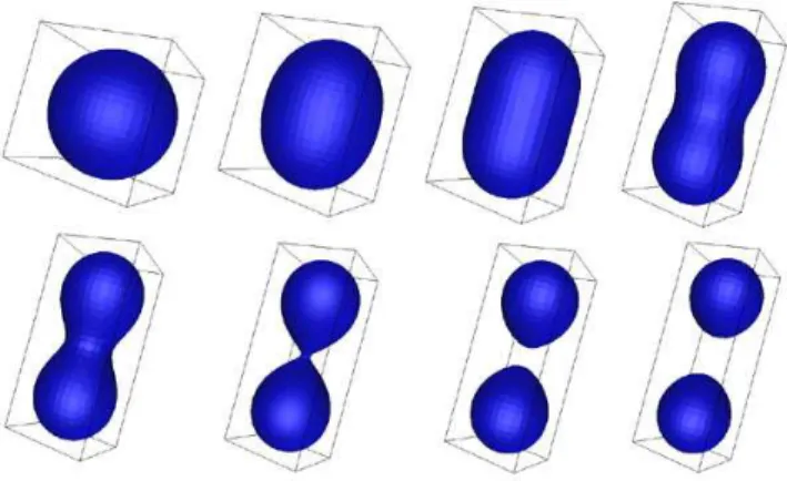
In this report, we will consider implicit functions which depend on time F (x, y, z, t). During the animation, the topology of the corresponding surface can change. Figure 4 illustrates an animated surface at different time.

1

(9)

Figure 4: an animated surface is splitting in two components

1.3 Morse Theory

As we said before, the implicit surface is defined by the set of points that satisfy F_{(x) = c where F : R}3

→ R and c is a constant. In this report, if F (x) ≥ c then x is inside the object2

, otherwise it is outside. Furthemore, the theory requires F to be C2

- continuous. In this way, we can define two notions: • the critical points of F occur where its gradient vanishes:

∇F (x) = (∂F ∂x(x), ∂F ∂y(x), ∂F ∂z(x)) = 0 • the Hessian H is defined as the Jacobian of the gradient:

H_{(x) = J(∇F (x)) =}    ∂2_F ∂x2(x) ∂2_F ∂x∂y(x) ∂2_F ∂x∂z(x) ∂2 F ∂y∂x(x) ∂2 F ∂y2(x) ∂ 2 F ∂y∂z(x) ∂2 F ∂z∂x(x) ∂2 F ∂z∂y(x) ∂2 F ∂z2(x)   

Morse Theory shows how the topology of the implicit surface is affected by the critical points. In the three dimensions case, we can classify the critical points of F and for each of these categories the corresponding topology change on the implicit surface. These cat-egories are summarized in the following table:

l1 l2 l3 Critical point

- - - Maximum

- - + 2-Saddle

- + + 1-Saddle

+ + + Minimum

Figure 5: Classification of critical points based on the sign of the 3 eigenvalues of the Hessian H(x)

2

(10)

2 Previous work

2.1 Ray-tracing

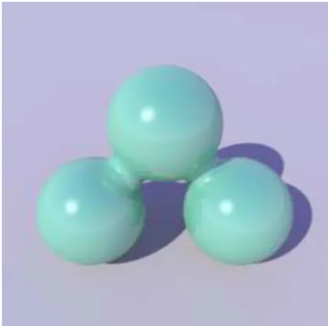
Several methods exist to display an implicit surface: the most accurate is ray-tracing, which consists in casting a ray for each pixel of the screen and computing the intersection with the surface. Figure 6 is an image obtained by the ray-tracing method.

Figure 6: Ray-traced metaballs rendered with POVRay

However, this method is not used for real-time applications but only for still images, because of its computational cost.

2.2 Marching cubes and particule-based methods

The preferred method is to represent the surface by a mesh, i.e. a set of connected triangles which approximate the surface. In this way, we just have to sample the surface by a number of points which could be determined by the user. This approach does not only permit a faster rendering, it is useful in other tasks, such as modeling or tracking surface features, as we will see later.

The common approach to sample the implicit surface is the marching cubes algorithm, which subdivides the space in voxels 3

, and for each of them, tests if the surface is in-tersecting it. Although it works fine for static surfaces 4_{, it is time-consuming and the}

topology of the resulting surface depends on the chosen resolution and does not corre-spond to the topology of the implicit surface. Furthemore, as the algorithm is launched at each frame for animated surfaces, there is no coherence between two meshes. Thus, it is impossible to follow a vertex from a frame to the next one. Finally, the resulting triangulation is not as regular5

as one could wish.

Other ways to sample the surface are particule-based and point-based methods: the idea is to start with an initial triangulation and convert each vertex into a particule and each edge into a spring linking two particles. The vertices evolve under the forces of the springs

3

a voxel is a volume element on a regular grid in three dimensional space

4

the parameters of the implicit function don’t vary in time

5

(11)

and are constrained on the implicit surface. In this way, the resulting mesh is only updated when the implicit function is animated. These two methods are illustrated in Figure 7.

Figure 7: (a)left Marching cubes algorithm (b)right Particule-based sampling

2.3 Dynamic triangulation of implicit surfaces

Antoine Bouthors and Matthieu Nesme proposed in [1] a particule-based triangulation method which uses the same mechanical properties as above.

The main difference is the use of two meshes:

• the mechanical mesh acts as an elastic surface and is computed by the Finite Elements Method (better than previous methods which use mass-spring systems). The main criterions for its design are robustness and speed. In addition to the mechanical part, some edges are collapsed or subdivided when they reach a certain length, to avoid bad quality and degenerate configurations. Then, the resulting mesh is more stable than previous approaches.

• the geometric mesh is only used for rendering purpose: it is generated by refining the mechanical mesh in areas of high curvature. The degree of accuracy can be controlled by the user.

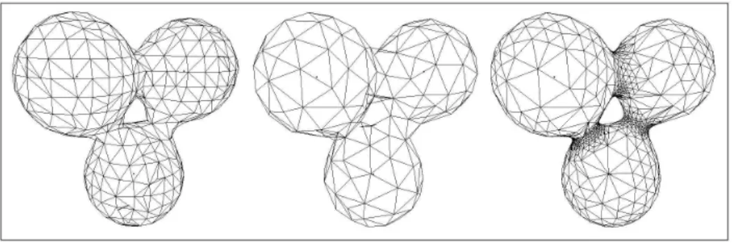
An initial triangulation is obtained by the marching cubes algorithm. Figure 8 sums up the different steps of the method.

(12)

Figure 8: (a)left initial marching cubes algorithm (b)middle mechanical mesh (c)right geometric mesh This method gathers many advantages since it provides robust, interactive and detailed rendering of animated or manipulated implicit surfaces.

2.4 Limitations

The method proposed by A. Bouthors and M. Nesme in [1] has some limitations: the animated implicit surfaces must have a constant topology, i.e. the number of connex com-ponents and the number of holes can not vary during the process. In the corresponding research report [2], they started some experiments that indicate it is possible to handle simple cases of blending and splitting. They concluded that it was possible to extend their method thanks to Stander & Hart works [3, 5]. The main goal of this intership was to allow dynamic triangulation of a wide range of implicit surfaces, including all the kinds of topology changes.

(13)

3 My contribution

Based on the Morse Theory presented in [3, 5], my work was then to detect the topology changes of the implicit surface and update the corresponding mesh in real-time.

3.1 Implementing Stander’s approach

To evaluate the method exposed in B. Stander’s thesis, I wrote my own implementation of the algorithms.

The method is composed of three parts: • Finding the critical points:

– an interval divide and conquer search algorithm with interval analysis is applied to the bounding box which contains the initial mesh

– when a box diameter reaches a given size, an interval Newton’s method is used to find the exact position of the critical points

• Tracking the critical points:

– the critical points velocities are computed by using the parameters velocities (or the skeleton points)

– the new locations of the critical points are approximated by a fourth-order Runge-Kutta

• Detecting and correcting topology changes on the mesh: – detecting a change in the sign of a critical value 6

– identifying polygons to remove and reconnecting the vertices of the removed poly-gons depending on the critical point’s variety

[3, 5] give some details about the algorithms and implementation tricks. Two new classes are created to manage interval arithmetics.

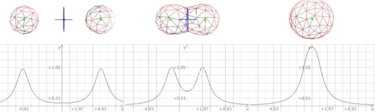
Experiments show that interval analysis method to find critical points is time-consuming, that is why the search is only processed at the beginning. It means that the algorithm does not account for new critical points that can be created spontaneously. Figure 9 is one of the several configurations where this case occurs.

6

(14)

Figure 9: (left) initially, there are 3 critical points: 2 maxima and a 2-saddle (middle-right) the 2 maxima disappear and the 2-saddle “becomes” a maximum

Moreover, the explicit expressions of the derivatives need to be known because of the interval analysis method: once more, it restricts the range of the implicit surfaces that we can consider.

3.2 Implementing surface tracking

Once the marching cubes algorithm is performed, initial 3D coordinates of all the mechanical mesh vertices are stored and they are used as texture coordinates. Thus, a 3D texture t(u, v, w) can be applied to the surface and when the vertices are moving, the texture is moving too since they keep the same texture coordinates during the animation. However, the number of vertices can vary because of some edge collapsing and refining. In this case, texture coordinates are modified as the following:

• edge collapse: texture coordinates of the remaining vertex is the average of the 2 initial 3D coordinates associated to the 2 old vertices which compose the collapsed edge

• edge refine: texture coordinates of the new vertex is the average of the 2 initial 3D coordinates associated to the 2 vertices which compose the refined edge

In this way, the animated surface and the texture applied to it have the same deformations. In fact, deformations such as projections of the vertices on the implicit surface are not considerate in this implementation.

3.3 Improvements over previous methods

3.3.1 Restricting the search

As noticed in Stander’s thesis [5], it is not possible to search for critical points at each frame because of performance issues with interval analysis.

Thus, it is necessary to restrict the search:

• the first idea is to look for critical points only in the neighborhood of the mesh ver-tices. Indeed, only critical points which are close to the surface are likely to modify the implicit surface’s topology. On the contrary, critical points far from the surface may have no influence on the topology of the surface, so they can be ignored without

(15)

any consequence.

• the second suggestion is to apply a standard Newton’s method to each vertex of the mechanical mesh instead of an interval analysis which is much more expensive. In addition, the implementation of analytic expressions of the partial derivatives is avoided. All computations are based on finite differences: for instance, instead of calculating ∂F

∂x analytically, we compute the approximation

∂F ∂x(x) ≈

F(x + h, y, z) − F (x, y, z) h

The same technique is used for all derivatives.

With this approach, it is possible to search for critical points at every time step in real-time. However, when the number of vertices increases, the program is slowing down because the algorithm’s complexity is O(nv) where nv is the number of vertices of the mechanical mesh.

The solution is to reduce the method to a small number of initial vertices. Indeed, our observations show that every vertex whose gradient’s norm reaches a local minimum is at the shortest distance to a critical point in space (this assumption needs to be demonstrated mathematically). The different steps of the algorithm are the following:

• for each vertex vi of the mechanical mesh, k∇F (vi)k is computed

• if one of the neighbour vertices vk of vi verifies k∇F (vi)k > k∇F (vk)k, then vi is not

a local minimum

• for each “local minimum” vertex, Newton’s method is applied

Figure 10 shows these particular vertices on two complex objects. Colored areas corre-sponds to the vertices of the mechanical mesh whose gradient norm is greater than the local minimum.

Figure 10: minima vertices (white) and their corresponding regions

The algorithm’s complexity is now O(ncp) where ncp is the number of critical points,

(16)

same as before, i.e. the number and the location of the critical points found with this algorithm are identical to a search using all the vertices.

3.3.2 Tracking critical points

The tracking of critical points is now straightforward: let F (x, t) and F (x, t + dt) be two configurations of the implicit function at time t and t + dt 7

. To know if the critical point cpi,t still exists at time t + dt, we proceed as the following:

• Newton’s method is applied to cpi,tat time t + dt (i.e. in F (x, t + dt) configuration):

let cpt+dt_i,t be the result. If the method diverges, then the critical point has probably disappeared, otherwise it means that cpi,t still exists

• at last, the search algorithm presented in section 3.3.1 is applied. Each time a critical point is found, a test is processed to know if we already found a critical point at this location. If it is not the case, we consider that a new critical point has appeared 3.3.3 Polygonization

When a critical value is changing sign, it means that the mechanical mesh needs to be modified in the neighbourhood of the critical point. Depending on its variety (extremum, 1-saddle, 2-saddle), the mesh is affected in different manners.

Let cpibe a critical point and vpi(t) its corresponding potential at time t. The implemented

algorithms are quite similar to those described in [3, 5]: • cpi is a maximum:

– vpi(t) < 0 and vpi(t + dt) > 0: a new component is created.

A bi-pyramid is centered on cpi: this new part of the mesh will fit the isosurface.

– vpi(t) > 0 and vpi(t + dt) < 0: a component is destroyed.

A ray is casted from cpi in any direction: the first hitted triangle takes part of

the component to be destroyed. • cpi is a 2-saddle:

– vpi(t) < 0 and vpi(t + dt) > 0: two components of the implicit surface are

connected.

A ray is casted from cpiin the eigenvector’s direction corresponding to the positive

eigenvalue. The two hitted triangles tri1 and tri2 are deleted and the vertices are

connected.

– vpi(t) > 0 and vpi(t + dt) < 0: a component is cut in two parts.

The plane defined by the two eigenvectors corresponding to the negative eigen-values hits a ring of triangles, they are deleted. The two rings of vertices are triangulated to repair the holes created.

• cpi is a 1-saddle. The algorithms are the same as the 2-saddle case.

7

in fact, t is the time when the nth

(17)

– vpi(t) < 0 and vpi(t + dt) > 0: a hole is spackled.

– vpi(t) > 0 and vpi(t + dt) < 0: a hole is pierced inside a component.

• cpi is a minimum. The algorithms are the same as the maximum case.

– vpi(t) < 0 and vpi(t + dt) > 0: a bubble disappears inside a component.

– vpi(t) > 0 and vpi(t + dt) < 0: a bubble appears inside a component.

Illustrations of these algorithms can be found in section 4.1.

3.4 Extension to discrete scalar fields

A discrete scalar field could be defined as:

F : [x0, x1] × [y0, y1] × [z0, z1] ⊆ N3 → R

As for continuous implicit functions, if F (n) ≤ c, n∈ N3_, _c_{∈ R, then n is inside the}

object, otherwise it is outside.

The isosurface (set of points such that F (n) = c) can be displayed in many different ways: as the function is not defined in some points of the space, an interpolation is used to compute the potential at these points. The trilinear interpolation was already implemented in the program, but it was not sufficient to find the critical points, because the resulting function ˜F is only C0_-continuous.

There are two possibilities to overcome this issue:

• Morse theory has been extended to discrete functions in [10, 11]

• a third degree Bezier interpolation gives a C2_{-continuous ˜}_F _{function: then, all the}

algorithms already presented can be applied to ˜F. I implemented this solution ([6, 8] give the details of how to find the 64 bezier coefficients)

Figure 11 shows a third degree Bezier interpolation of a discrete scalar field provided by a fluid simulation.

(18)

4 Results and limitations

4.1 Topology changes and Surface tracking

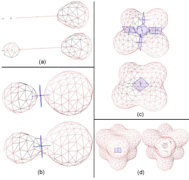
All the possible topology changes are handled in the application: an exhaustive list of the different cases can be seen on Figure 12.

Figure 12: (a)destroy-create (b)detach-connect (c) pierce-spackle (d) burst-bubble The user has the possibility to create an initial scene by placing two kinds of skeleton elements (points and lines) in space, defining a radius for each of them, and many other features.

(19)

and geometric meshes are updated in real-time: for instance, a scene including 7 metaballs which connect each other is running with 25 frames per second, while a more complex scene with 60 metaballs is decreasing the framerate to 4. This is due to the higher cost of evaluating F (x). Furthemore, there is no lag during topology changes because the complexity of the polygonization algorithms is insignificant in comparison to the rest of the program.

A perlin noise 8 _shader9 _{is applied to the mesh to show that it is possible to track the}

surface, i.e. to follow the move of any point on the implicit surface. Figure 13 is an exemple of 2 metaballs splitting, textured with this shader.

Figure 13: two components are splitting : perlin noise shader applied

4.2 Limitations and possible improvements

Some stability problems can arise when the implicit surface is too thin, because the neighbouring vertices may be projected to the wrong side of the isosurface, which results in triangle inversions. Some attempts have been made to avoid this case, such as collapsing inverted and/or bad quality triangles, without success. Finally, I found a solution that significantly increases the stability when the mechanical computations are off. For each couple of faces, the following process is performed:

• compute the difference between the angles of the two face normals

• compute the difference between the angles of the two gradients choosed at triangles barycenters

• if the difference between these two values is greater than a given threshold, the com-mon edge is swapped10

8

It resulted from the work of Ken Perlin. Perlin noise is a procedural texture primitive and is widely used in computer graphics for effects like fire, smoke, and clouds

9

a shader is a part of the renderer, which is responsible for calculating the color of an object. Shaders are processed within the Graphics Processing Unit (GPU) of the computer

10

(20)

Sometimes, the algorithm does not detect that a critical value has changed sign, for some reasons (for instance, the critical point is detected when it has already changed sign). When it happens, the mesh does not match the topology of the implicit surface anymore, which results in many incoherences, and there is no way to recover a well-shaped mesh. To avoid this unwanted situation, an alternative is to expand the search area when applying Newton’s method, in order to find more critical points.

Newton’s method for critical points search is restricted to vertices whose gradient’s norm reaches a local minimum. However, some experimentations indicate that in the case where the mechanical mesh is not enough refined, these particular vertices are fewer than critical points. This seems to be a discretization issue. For now, mesh refinement is the only solution.

In this work, we assumed that the eigenvalues of the Hessian are all non-zero, but in rare situations, one of them vanishes. It often occurs when the dimension of the critical set is greater than zero (i.e. it is a critical line, plane or volume). In such a case, topology changes detection is not valid anymore because Morse Theory can not be applied: the algorithm finds many critical points which are in fact contained in a higher dimensional critical set.

At last, in a scene using metaballs, it could be possible to only update the part of the mesh that is influenced by the skeleton’s modifications: indeed, when the user is moving one geometric element, it is worthless to recompute the location of the vertices which are further than the current element’s radius: there are many existing data structures and algorithms (e.g. octrees) that can be used to speed the computations on complex scenes.

(21)

Conclusion

This internship was very enriching to me since I had the opportunity to improve my knowledge in computer graphics as well as my coding experience: it allowed me to apply numerical methods and to discover a very specialized field, Morse theory and topology on implicit surfaces. I have learnt the state of the art in this field by reading many articles and research report. In a more practical point of view, I also learned how to use the fundamental Application Programming Interface OpenGL and the shader programmation: indeed, before to begin the research part, I needed to read, understand and restructure the program.

The obtained results are quite satisfying since the main limitations have been overcomed. In a future work, this method could be applied to more general implicit surfaces such as discrete scalar fields to display textured fluid simulations. Furthemore, stability problems have to be solved to make this method usable.

Finally, I would like to thank my supervisors for their support during the training period and for their great ideas.

(22)

References

[1] A.Bouthors, M. Nesme. Twinned Meshes for Dynamic Triangulation of Implicit Surfaces. Graphics Interface, 2007.

[2] A.Bouthors, M. Nesme. Dynamic Triangulation of Implicit Surfaces: towards the handling of topology changes. INRIA, November 2006.

[3] B. Stander, J. Hart. Guaranteeing the Topology of an Implicit Surface Polygonization for Inter-active Modeling. SIGGRAPH, 1997.

[4] J. Hart, A. Durr, D. Harsh. Critical Points of Polynomial Metaballs. Implicit Surfaces, 1998. [5] Stander, B. T. Polygonizing Implicit Surfaces with Guaranteed Topology. PhD thesis, School of

EECS, Washington State University, May 1997.

[6] C. L. Bajaj. Modeling Physical Fields for Interrogative Visualization Department of Computer Sciences, Purdue University, West Lafayette, Indiana, 1997

[7] A. Bottino, W. Nuij and K. van Overveld. How to Shrinkwrap through a Critical Point: an Algorithm for the Adaptive Triangulation of Iso-Surfaces with Arbitrary Topology. Department of Mathematics and Computing Science, Eindhoven University of Technology, 1996.

[8] C. L. Bajaj, V. Pascucci. Visualization of Scalar Topology for Structural Enhancement. Depart-ment of Computer Sciences and TICAM, University of Texas, Austin, 1998.

[9] Wu, Shin-Ting, M. de G. Malheiros. On Improving the Search for Critical Points of Implicit Func-tions. Image Computing Group (GCI/DCA/FEEC), State University of Campinas, Sao Paulo, Brazil, 1999.

[10] G. H. Weber, G. Scheuermann, H. Hagen, B. Hamann. Exploring Scalar Fields Using Critical Isovalues. University of Kaiserslautern, Germany and Dept. of Computer Science, University of California, Davis, U.S.A., 2002.

[11] A. Zomorodian, J. Harer, H. Edelsbrunner. Hierarchical Morse Complexes for Piecewise Linear 2-Manifolds. Dept. of Computer Science, University of Illinois, and Department of Mathematics, Duke University, North Carolina, 2001.

[12] P. Bourke. Implicit Surfaces, also known as ”Metaballs”, ”Blobbies”, ”Soft objects”. http://ozviz.wasp.uwa.edu.au/˜pbourke/modelling rendering/implicitsurf, June 1997.

[13] Adam W. Bargteil, Tolga G. Goktekin, James F. O’Brien, and John A. Strain. A Semi-Lagrangian Contouring Method for Fluid Simulation. University of California, Berkeley, 2006.

[14] P. P. Pebay, T. J. Baker. Analysis Of Triangle Quality Measures. Mahtematics Of Computation, Volume 72, Number 244, Pages 1817-1839, 2003.

[15] D. Ratz. Box-Splitting Strategies for the Interval Gauss-Seidel Step in a Global Optimization Method. Computing, 53, 337-353, Karlsruhe, 1994.

[16] A. Witkin, P. Heckbert. Using Particles to Sample and Control Implicit Surfaces. SIGGRAPH, 1994.