Research Article
Predicting Financial Extremes Based on Weighted Visual
Graph of Major Stock Indices
Dong-Rui Chen,
1Chuang Liu ,
1Yi-Cheng Zhang,
1,2and Zi-Ke Zhang
1,31Alibaba Research Center for Complexity Sciences, Hangzhou Normal University, Hanghzou 311121, China 2Department of Physics, University of Fribourg, Fribourg 1700, Switzerland
3College of Media and International Culture, Zhejiang University, Hangzhou 310028, China
Correspondence should be addressed to Chuang Liu; [email protected] and Zi-Ke Zhang; [email protected] Received 3 June 2019; Revised 20 August 2019; Accepted 23 September 2019; Published 31 October 2019
Academic Editor: Lucia Valentina Gambuzza
Copyright © 2019 Dong-Rui Chen et al. This is an open access article distributed under the Creative Commons Attribution License, which permits unrestricted use, distribution, and reproduction in any medium, provided the original work is properly cited.
Understanding and predicting extreme turning points in the financial market, such as financial bubbles and crashes, has attracted much attention in recent years. Experimental observations of the superexponential increase of prices before crashes indicate the predictability of financial extremes. In this study, we aim to forecast extreme events in the stock market using 19-year time-series data (January 2000–December 2018) of the financial market, covering 12 kinds of worldwide stock indices. In addition, we propose an extremes indicator through the network, which is constructed from the price time series using a weighted visual graph algorithm. Experimental results on 12 stock indices show that the proposed indicators can predict financial extremes very well.
1. Introduction
The stock market is an important part of global financial markets. Since entering the stock market is relatively easy and the returns are considerable, the stock market has be-come a major market for investment activities of ordinary investors. However, compared with the capital markets of developed countries such as the United States, emerging stock markets, as represented by China, are more volatile, and their system risks are much greater, due to the short establishment time and imperfect institutional system. Therefore, modelling the stock market and making accurate predictions are very useful for both investors and regulatory authorities to manage the system risk [1]. The financial extremes, such as bubbles, crashes, and rebounds, play a crucially important role in research of the stock market, and prediction of financial extremes using stock market indices is also a hot topic in the research of financial markets [2–4]. In the last decade, there has been a growing body of literatures addressing the utilization of complex network methods for the characterization of dynamical systems based on time series. There are at least three main class approaches
to transform time series to network representations [5], such as proximity networks [6], transition networks [7], and visibility graphs [8]. The connectivity of proximity networks is determined by the mutual statistical similarity or metric proximity between different segments of a time series. Zhang and Small introduced a method to convert the pseudo-periodic time series into networks, in which cycles in the time series are considered nodes, and the edges are de-termined by the strength of temporal correlation between cycles [6]. Xu et al. proposed another method in which phase-space points are considered nodes in the network, and each node links to its closest k neighbors to form a complex network [9]. To produce an ordinal partition transition network, the time series is symbolized using ordinal pat-terns. The ordinal patterns are used as the nodes of the network, and directed edges are based on temporal suc-cession of the ordinal patterns [10]. The visibility graph algorithm was proposed by Lacasa in 2008, in which nodes correspond to the data points of the time series, and an edge is assigned to connect two nodes if they can see each other. The visibility graph algorithm can map all types of time series into networks, by converting a periodic series into a Volume 2019, Article ID 5320686, 17 pages
regular graph, a random series into a random graph, and a fractal sequence into a scale-free network [8, 11–14].
Based on the visibility framework, a horizontal visibility algorithm [15] and a limited penetrable visibility algorithm were generated [16]. Stephen et al. extracted all the segments in a time series with a predefined window size and mapped each segment to a visibility graph. The successively occurring visibility graphs are linked in turn. The weights of links reflect the transfer behaviors of the distinguishable states [17]. In addition, Yan and Serooskerken proposed an ab-solute invisibility graph, which is just the opposite of the visibility algorithm, to predict the trough points in the stock prices [18]. For the low complexity and good geometric properties, the visibility graph has been widely applied in many kinds of time series, including turbulence [19], sun-spot series [20], electrocardiograms (ECGs) [21], the Con-struction Cost Index (CCI) [22, 23], and financial market [24–28].
Based on the previous achievements, we constructed a weighted visual graph (including the visibility graph and absolute invisibility graph), in which the edge weight is defined as the combination of the price difference and the time interval of the corresponding nodes. We then proposed a new predictive indicator of the financial extremes based on the weighted visual graph. The extremes of the financial market are defined as the peak (or trough) points, which are the maximum (or minimum) index among a period of stock prices in this paper. Experiments on 12 indices show the strong predictive power of the proposed indicators.
The rest of this paper is organized as follows. In Section 2, we describe the data used in this work and propose the indicators of financial extremes. In Section 3, we show the experimental results on 12 stock indices. Conclusions are drawn in Section 4.
2. Methodology and Data Description
2.1. Data Description. A series of stock market indices can
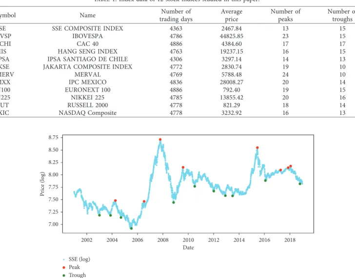
reflect the overall movement of the markets. We collected 12 major stock market indices from Yahoo Finance (https:// finance.yahoo.com) and used the daily closing price series for approximately 19 years, from January 2000 to December 2018. During this period, there were about 4500 trading days (the accurate trading days may be slightly different between the indices). The extremes (peak or trough points) of the financial market are defined as the maximum (or minimum) index within a period of stocks. Table 1 shows the in-formation and the basic statistic of the 12 stock indices, where a � 45 and b � 131 (these variables will be explained later). In this work, we propose an indicator of the extremes on these datasets.
2.2. Problem Definition. In this study, we define the extremes
of the financial market as the peak (or trough) points that are the maximum (or minimum) index within a period of stocks. In this case, we aim to find an indicator that has strong predictive power for the peak (or trough) points. Mathematically, for a given stock price time series (t, y),
where t is the time variable and y the price value at t, the point at time t is a peak (or trough) point if yt is the
maximum (or minimum) price over the period of (t − b, t + a), where a and b are the number of trading days after (a) and before (b) the current day, respectively. As in the previous work [18], we chose b � 131 and a � 45, which denote the number of trading days in 6 months and 2 months, respectively. In total, the numbers of peak and trough points for each stock index in the considered period are illustrated in Table 1. Figure 1 illustrates the peak and trough points of the Shanghai Stock Exchange (SSE) index. Our goal in this work is to predict whether the peak (or trough) points will appear in the next several days.
2.3. Construction of Visibility Graph and Absolute Invisibility Graph
2.3.1. Visibility Graph. In this work, we find the indicator of
extremes from the network perspective, but first we briefly introduce the visibility graph algorithm proposed by Lacasa et al., which is the most commonly used method to convert a time series into a network [8]. For a series (t, y), a visible edge exists between two nodes (ti, yi) and (tj, yj), if any
node (tk, yk)located between them satisfies
yk< yi+
tk− ti
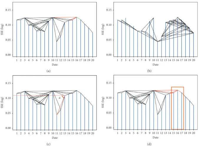
tj− tiyj− yi, ∀i < k < j. (1) Figure 2(a) is a schematic of the visibility graph that was converted from the series of SSE index’s daily closing prices in January 2015. A natural number is used to mark the trading days. The points and lines between them constitute the visibility graph. The nodes correspond to series data in the same order and an edge connects two nodes if one can see the other (visibility between them). Taking points 10 and 16 of Figure 2(a) as the example with which to explain the concept of “visibility,” between points 10 and 16 there are five points (11 to 15) that are all under the red line from point 10 to 16. A link (visibility) exists between nodes 10 and 16. As the definition of the visibility graph, the node with a large price would be more likely to have more links, and this would be the basic method with which to predict the peak points.
2.3.2. Absolute Invisibility Graph. The absolute invisibility
graph algorithm [18] is just the opposite of the visibility algorithm. For a series (t, y), an absolute invisibility edge exists between two nodes (ti, yi) and (tj, yj), if any node
(tk, yk)located between them satisfies
yk> yi+
tk− ti
tj− ti
yj− yi
, ∀i < k < j. (2)
Figure 2(b) is a schematic of the absolute invisibility graph. Taking points 12 and 16 of Figure 2(b) as an example with which to explain the concept of “absolute invisibility,” between points 12 and 16 there are three points (13, 14, and 15) that are all above the line from points 12 to 16. Therefore, every point located in 12 and 16 can obstruct the visibility between 12 and 16, and a link (absolute invisibility) exists. As
the definition of the absolute invisibility graph, the node with a low price would be more likely to have more links, and this would be the basic method with which to predict the trough points.
Based on the visibility graph and absolute invisibility graph algorithm, Yan and Serooskerken put forward an indicator to predict the extreme value in the time series [18]. The method in their article shows there will be more possible appearances of an extreme value if the degree of the cor-responding node is much higher than the others.
2.4. Indicator of Extremes. It should be noted that the above
methods consider only the edge between two nodes, which misses a lot of detailed information of the original series. Taking the visibility graph as an example (Figure 2(a)), the link between points 11 and 12 and that between points 11 and 13 have no differences in the original visibility graph. However, the difference of the variation (|y12− y11|
versus|y13− y11|) is very significant, which is also an
im-portant factor related to the extremes. Therefore, we propose a weighted visual graph (WVG), which considers the
variation between the two points based on the original visibility graph or absolute invisibility graph. As shown in Figure 2(c), the dotted line represents the horizontal sight line, and the angle between the solid line and the dotted line is defined as the depression angle. For a pair of nodes that satisfy the visual condition of the visibility graph (or absolute invisibility graph), the weight of the edge between them is defined as the tangent value of the depression angle:
wij �tan αij�
yj− yi
tj− ti
. (3)
Compared with the original visibility graph (or absolute invisibility graph) algorithm, the WVG algorithm considers more details such as the time interval and price variation between two points in the time series. It should be noted that, if the price increased, the depression angle is positive, leading to positive weight, and vice versa. Among the entire time series, we use the observation window with S days of data to construct the weighted visual graph. For each graph converted from the corresponding time window, we define
Piw and Tiw for the weighted visual graph as the indicator
Table 1: Index data of 12 stock indices studied in this paper.
Symbol Name trading daysNumber of Averageprice Number ofpeaks Number oftroughs
SSE SSE COMPOSITE INDEX 4363 2467.84 13 15
BVSP IBOVESPA 4786 44825.85 23 15
FCHI CAC 40 4886 4384.60 17 17
HIS HANG SENG INDEX 4763 19237.15 16 15
IPSA IPSA SANTIAGO DE CHILE 4306 3297.14 14 13
JKSE JAKARTA COMPOSITE INDEX 4772 2830.74 19 10
MERV MERVAL 4769 5788.48 24 10
MXX IPC MEXICO 4836 28008.27 20 14
N100 EURONEXT 100 4886 792.40 19 15
N225 NIKKEI 225 4785 13855.42 20 16
RUT RUSSELL 2000 4778 821.29 18 14
IXIC NASDAQ Composite 4778 3232.92 16 13
8.75 8.50 8.25 Price (log) 2002 2004 2006 2008 2010 Date 2012 2014 2016 2018 8.00 7.75 7.50 7.25 7.00 SSE (log) Peak Trough
Figure 1: Peak (red) and trough (green) points of the Shanghai Stock Exchange (SSE) index. Blue curve represents the price index (a � 45 and b � 131).
with which to predict the appearance of the peak and trough points in the following days, respectively. To predict the peak points, we use the weighted visibility graph, and Pi
w is de-fined as Piw i− 1 j i− Swij S− 1 . (4)
To predict the trough points, we use the weighted ab-solute invisibility graph, and Ti
w is defined as
Tiw −
i− 1
j i− Swij
S− 1 , (5)
where i represents the rightmost point in the observing window and S is the length of the observation window.
For the weighted visual graph, the structure of each node is very sensitive to the neighborhood values. Affected by the neighbors, the indicators based on the visibility graph and absolute invisibility graph fluctuate frequently. For example, according to Figures 2(a) and 2(b), it is obvious that, for the points 16 and 17, although these two days’ prices are similar, the corresponding indicators are very different. To reduce the impact of neighbor points, we consider the observations’ neighbor nodes as a whole (as shown in Figure 2(d)), and the accumulated weighted indicators can be calculated as follows: Picw i k i− n+1 k− 1 j k− Swkj/(S − 1) n , (6) Ticw − i k i− n+1 k− 1 j k− Swkj/(S − 1) n , (7)
where n decides the size of the considered accumulated neighbors.
3. Results and Discussions
3.1. Comparison Methods. Indicators that are based on the
degree (D) and accumulated degree (AD) of the visibility graph and absolute invisibility graph are applied as the comparison methods. The indicators used in this work are summarized in Table 2.
3.2. Metrics. We set the observation window with a length of
262 (S 262) trading days, and its moving step equals 1 day. For each observation window, we calculate the indicators listed in Table 2, and we expect that the peak point (or trough point) would appear in the following 45 (a 45) days if the indicator is significant. Therefore, we choose different thresholds for the indicators to observe the predictions.
8.15 8.10 8.05 SS E (log) 8.00 1 2 3 4 5 6 7 8 9 10 11 12 13 14 15 16 17 18 19 20 Date (a) 8.15 8.10 8.05 SS E (log) 8.00 1 2 3 4 5 6 7 8 9 10 11 12 13 14 15 16 17 18 19 20 Date (b) 8.15 8.10 8.05 SS E (log) 8.00 1 2 3 4 5 6 7 8 9 10 α Date 11 12 13 14 15 16 17 18 19 20 (c) 8.15 8.10 8.05 SS E (log) 8.00 1 2 3 4 5 6 7 8 9 10 Date 11 12 13 14 15 16 17 18 19 20 (d)
Figure2: Schematic of four different algorithms: (a) visibility algorithm; (b) absolute invisibility algorithm; (c) weight based on angle; (d) accumulated neighbors.
Once the indicator value is above the threshold, we believe that there will be a peak (or a trough) point within 45 days after the rightmost point of the corresponding window. To test the performance of the proposed indicators, we calculate the precision (P) and recall (R) separately. Supposing that Ne
is the number of the extremes (peak or trough points) in the total time series, Np is the number of the prediction
ex-tremes in which the indicator values are larger than the threshold and Ntpis the number of the prediction extremes,
which are the real extremes. Precision can be obtained through precision � (Ntp/Np) and recall through
recall � (Ntp/Ne). Large precision means the high accuracy
of the method and large recall means more extremes are predicted. While precision and recall are two competitive measures of performance, we use F1 score as the major measurement. F1 score is defined as follows:
F1 �2 ∗ precision ∗ recall
precision + recall . (8)
3.3. Experimental Results. First, we take the SSE index case as
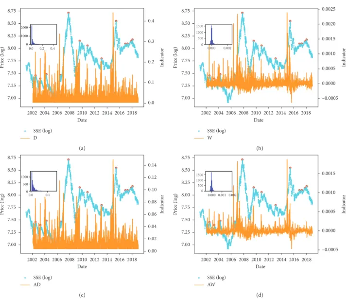
an example to illustrate the prediction process. For each ob-servation time window, we can obtain an indicator according to the equations listed in Table 2. Figures 3 and 4 show the distribution of the indicators based on various methods for the peak and trough point, respectively. The yellow bars represent the indicator value, and the blue dots are the index’s price (log) series. It should be noted that the indicator for the first year cannot be calculated, as the window size is equal to 262 (approximately 1 year). According to both figures, there will always be a significantly large indicator before the peak (or trough) points, which shows that all the indicators are valid for predicting the extremes. However, comparing the indicators based on node degree (VG, Figures 3(a) and 4(a)) and edge weights (WVG, Figures 3(b) and 4(b)), the indicator values based on the edge weights more clearly detect the significant indicators, in which most of the indicators are rounded to 0 and very few indicator values are very large, which are in-timately related to the peak (or trough) points.
We focused on a particular extreme (financial crash) during 2014 to 2016 in the SSE as an example to show the interaction of the extreme events and indicators. Figure 5 shows the partial process of the formation and collapse of the corresponding SSE index bubble. In late November 2014, the SSE index began to rise gradually due to macroeconomic expectations and loose monetary policy. During December 2014 to January 2015, the SSE index rose from 2680 to 3210
(nearly 20%), which is obviously a faster-than-exponential growth of prices. Thus, we can confirm that a bubble was forming. According to Figure 5(a), it can be seen that the fluctuation of the peak indicator increased sharply in this period, and the maximum value of the peak indicator appeared on December 8, 2014. After the peak indicator reached the maximum, the SSE index continued to rise, and the stock market risk was further increased. Meanwhile, the financial regulatory authorities took some more stringent measures, and the increase stopped at 5166 on June 12, 2015. In the following two natural months, the SSE index fell by more than 42%, a faster-than-exponential decrease. There was a significant negative bubble at this stage. The trough indicators constructed in this work also fully reflect the process. As shown in Figure 5(b), in the negative bubble stage, the trough prediction indicator increased rapidly. In late August 2015, the trough indicator fluctuated sharply. On August 26, the lowest point was 2927.29 and the trough indicator reached a corresponding minimum. From Figure 5(a), we note that the peak indicators also decreased during the negative bubble process, but the changes of the trough indicators are more sensitive.
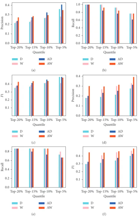
To test the performance of the proposed method, we show the precision, recall, and F1 score for peak and trough prediction in Figure 6. For the accumulated methods, the number of neighbors is set as n � 3. The horizontal axis represents different thresholds of the indicators, where the indicator with a value larger than the threshold indicates peak (or trough) points in the following 45 trading days. As the indicator via different methods shows a significant difference (according to Figures 3 and 4), it would be difficult to use the concrete values to interpret the threshold. Here, we use the percentages to represent the threshold in Figure 6. For example, the top 20% indicates that the top 20% indicators are treated as the extreme indicators. For various thresholds, we can observe that the precision increases with increasing threshold (Figures 6(a) and 6(d)) because of too many false-positive samples with a small threshold. A similar phenomenon has also been discovered in other forecasting scenarios, such as recom-mendation systems [29] and link prediction in social networks [30]. It is interesting to find that the recall is very high (nearly 100%) even with very high threshold of the indicator value, which means that almost all the real ex-tremes (peak and trough points) can be forecast by the indicators. According to Figure 6, one can find that the indicators, through accumulated weights on WVG (red bars, Pcw (or Tcw)), are more accurate than the other
Table 2: Summary of indicators.
Peak indicators (visibility graph) Trough indicators (absolute invisibility graph)
Degree (D) Pi
d� di Tid� di
Accumulated degree (AD) Pi
cd� i k�i− n+1(dk/n) T i cd� i k�i− n+1(dk/n) Weight (W) Pi w� ( i−1 j�i− Swij/(S − 1)) Tiw� − ( i−1 j�i− Swij/(S − 1))
Accumulated weight (AW) Pi
cw� i k�i− n+1( k−1 j�k− Swkj/(S − 1))/n T i cw� − i k�i− n+1( k−1 j�k− Swkj/(S − 1))/n
diis the degree of node i, wijis the weight of node pair (i, j), S is the length of the observation window, n is the number of considered neighbors, and i is the
8.75 8.50 2000 1000 0.0 0.2 0.4 0 8.25 8.00 7.75 Pr ice (log) 7.50 7.25 7.00 0.4 0.3 0.2 0.1 0.0 In dica to r 2002 2004 2006 2008 2010 2012 Date 2014 2016 2018 SSE (log) D (a) 1000 1500 500 0 0.000 0.002 8.75 8.50 8.25 8.00 7.75 –0.0005 0.0000 0.0005 0.0010 0.0015 0.0020 0.0025 Pr ice (log) In dica to r 7.50 7.25 7.00 2002 2004 2006 2008 2010 2012 Date 2014 2016 2018 SSE (log) W (b) 1000 500 0.0 0.1 0 8.75 8.50 8.25 8.00 7.75 Pr ice (log) 7.50 7.25 7.00 0.14 0.12 0.10 0.08 0.06 0.04 0.02 0.00 In dica to r 2002 2004 2006 2008 2010 2012 Date 2014 2016 2018 SSE (log) AD (c) 1000 1500 500 0 0.000 0.001 0.002 8.75 8.50 8.25 8.00 7.75 Pr ice (log) 7.50 7.25 7.00 –0.0005 0.0000 0.0005 0.0010 0.0015 In dica to r 2002 2004 2006 2008 2010 2012 Date 2014 2016 2018 SSE (log) AW (d)
Figure3: Peak indicators based on different methods on the Shanghai Stock Exchange (SSE) index series. Yellow bars represent the indicator values, blue dots the original index price series, and red circles the real peak points. Inset shows the indicator distribution. (a) Degree (D) indicator; (b) weight (W) indicator; (c) accumulated degree (AD) indicator; (d) accumulated weight (AW) indicator (a 45,
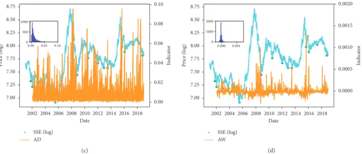
b 131, and S 262). 8.75 8.50 1000 1500 0.0 0.2 0 500 8.25 8.00 7.75 Pr ice (log) 7.50 7.25 7.00 0.15 0.20 0.25 0.10 0.05 0.00 In dica to r 2002 2004 2006 2008 2010 2012 Date 2014 2016 2018 SSE (log) D (a) 1000 2000 0 0.000 0.001 0.002 8.75 8.50 8.25 8.00 7.75 0.0000 0.0005 0.0010 0.0015 0.0020 Pr ice (log) In dica to r 7.50 7.25 7.00 2002 2004 2006 2008 2010 2012 Date 2014 2016 2018 SSE (log) W (b) Figure4: Continued.
1000 500 0.00 0.05 0.10 0 8.75 8.50 8.25 8.00 7.75 Pr ice (log) 7.50 7.25 7.00 0.10 0.08 0.06 0.04 0.02 0.00 In dica to r 2002 2004 2006 2008 2010 2012 Date 2014 2016 2018 SSE (log) AD (c) 1000 2000 0 0.000 0.001 8.75 8.50 8.25 8.00 7.75 Pr ice (log) 7.50 7.25 7.00 0.0000 0.0005 0.0010 0.0015 0.0020 In dica to r 2002 2004 2006 2008 2010 2012 Date 2014 2016 2018 SSE (log) AW (d)
Figure4: Trough indicators based on different methods on the Shanghai Stock Exchange (SSE) index series. Yellow bars represent the indicator values, blue dots the original index price series, and green circles the real trough points. Inset shows the indicator distribution. (a) Degree (D) indicator; (b) weight (W) indicator; (c) accumulated degree (AD) indicator; (d) accumulated weight (AW) indicator (a 45,
b 131, and S 262). 8.75 8.6 8.4 8.2 0.0015 0.0010 0.0005 0.0000 8.0 7.8 7.6 2014-072014-092014-112015-012015-032015-052015-072015-092015-112016-012016-03 8.50 8.25 8.00 7.75 Pr ice (log) 7.50 7.25 7.00 2002 2004 2006 2008 2010 2012 Date 2014 2016 2018 0.0020 0.0015 0.0010 0.0005 0.0000 In dica to r SSE (log) AW (a) 0.0010 0.0005 0.0000 8.6 8.4 8.2 8.0 7.8 7.6 2014-072014-092014-112015-012015-032015-052015-072015-092015-112016-012016-03 8.75 8.50 8.25 8.00 7.75 Pr ice (log) 7.50 7.25 7.00 2002 2004 2006 2008 2010 2012 Date 2014 2016 2018 0.0015 0.0010 0.0005 0.0000 In dica to r 0.0015 SSE (log) AW (b)
methods both in the prediction of peak and trough points. In addition, for various thresholds, the improvements are still robust.
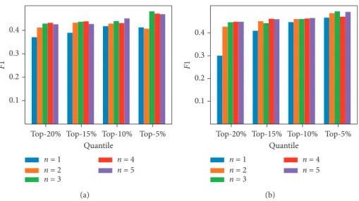
Figure 6 indicates that the indicators based on the accumulated weight on WVG are the best way to predict the extremes on the SSE index series. For the calculation of
Pcw (or Tcw), we must set the number of considered
neighbors (n). Figure 7 illustrates the influence of n on the prediction accuracy, and the bar represents the F1 score. It should be pointed out that n 1 is just Pw (or Tw) that
does not consider the neighbors’ influence. Figure 7 shows that the F1 score is very different between n 1 and n > 1, but the increment varies slightly with increasing when
n> 1. This indicates that the influence of n is not very significant, but considering the neighbors’ influence is very important.
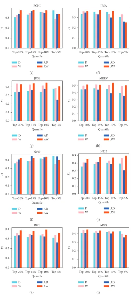
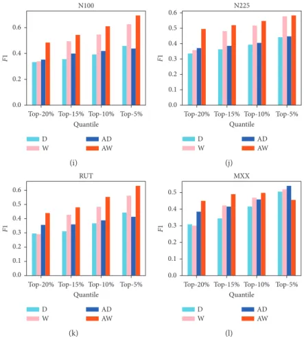
We check the performance of the proposed indicators on 12 major financial indices. Figures 8 and 9 present the F1 scores for the four indicators of peak and trough points, respectively. Similar to the result of the SSE, the indicators
D W ADAW Pr ecisio n 0.4 0.3 0.2 0.1 0.0
Top-20% Top-15% Top-10% Top-5% Quantile (a) D W ADAW Recall 0.8 1.0 0.6 0.4 0.2 0.0
Top-20% Top-15% Top-10% Top-5% Quantile (b) D W ADAW F1 0.4 0.3 0.2 0.1
Top-20% Top-15% Top-10% Top-5% Quantile (c) D W ADAW Pr ecisio n 0.4 0.3 0.2 0.1 0.0
Top-20% Top-15% Top-10% Top-5% Quantile (d) D W ADAW Recall 0.8 0.6 0.4 0.2 0.0
Top-20% Top-15% Top-10% Top-5% Quantile (e) D W ADAW F1 0.4 0.3 0.2 0.1
Top-20% Top-15% Top-10% Top-5% Quantile
(f)
Figure6: Performance of extreme indicators according to different methods on the Shanghai Stock Exchange (SSE) index series. (a) Precision for peak prediction; (b) recall for peak prediction; (c) F1 score for peak prediction; (d) precision for trough prediction; (e) recall for trough prediction; (f) F1 score for trough prediction (a 45, b 131, and S 262).
0.3 0.4
0.2 0.1
F1
Top-20% Top-15% Top-10% Quantile Top-5% n = 1 n = 2 n = 3 n = 4 n = 5 (a) 0.3 0.4 0.2 0.1 F1
Top-20% Top-15% Top-10% Quantile Top-5% n = 1 n = 2 n = 3 n = 4 n = 5 (b)
Figure7: Influence of n for indicator through accumulated WVG on prediction performance (a 45, b 131, and S 262).
SSE 0.4 0.5 0.3 0.2 F1 0.1 0.0
Top-20% Top-15% Top-10% Quantile Top-5% D W AD AW (a) IXIC 0.3 0.2 0.1 0.0 F1
Top-20% Top-15% Top-10% Quantile Top-5% D W AD AW (b) HSI 0.5 0.6 0.4 0.3 0.2 F1 0.1 0.0
Top-20% Top-15% Top-10% Quantile Top-5% D W AD AW (c) 0.5 0.6 0.4 0.3 0.2 F1 0.1 0.0
Top-20% Top-15% Top-10% Quantile Top-5% BVSP D W AD AW (d) Figure8: Continued.
FCHI 0.3 0.2 0.1 0.0 F1
Top-20% Top-15% Top-10% Quantile Top-5% D W AD AW (e) IPSA 0.3 0.2 0.1 0.0 F1
Top-20% Top-15% Top-10% Quantile Top-5% D W AD AW (f) JKSE 0.3 0.4 0.2 0.1 0.0 F1
Top-20% Top-15% Top-10% Quantile Top-5% D W AD AW (g) MERV 0.5 0.4 0.3 0.2 F1 0.1 0.0
Top-20% Top-15% Top-10% Quantile Top-5% D W AD AW (h) N100 0.3 0.4 0.2 0.1 0.0 F1
Top-20% Top-15% Top-10% Quantile Top-5% D W AD AW (i) N225 0.5 0.4 0.3 0.2 F1 0.1 0.0
Top-20% Top-15% Top-10% Quantile Top-5% D W AD AW (j) RUT 0.3 0.4 0.2 0.1 0.0 F1
Top-20% Top-15% Top-10% Quantile Top-5% D W AD AW (k) MXX 0.3 0.4 0.2 0.1 0.0 F1
Top-20% Top-15% Top-10% Quantile Top-5% D W AD AW (l)
Figure8: Performance of peak indicators based on four methods for 12 indices. The x axis is the threshold selected during prediction of extreme values and the y axis is the F1 score (a 45, b 131, S 262, and n 3 (for accumulated degree (AD) or accumulated weight (AW))).
SSE 0.4 0.5 0.3 0.2 F1 0.1 0.0
Top-20% Top-15% Top-10% Quantile Top-5% D W AD AW (a) IXIC 0.6 0.4 0.2 0.0 F1
Top-20% Top-15% Top-10% Quantile Top-5% D W AD AW (b) HSI 0.5 0.6 0.4 0.3 0.2 F1 0.1 0.0
Top-20% Top-15% Top-10% Quantile Top-5% D W AD AW (c) 0.5 0.6 0.4 0.3 0.2 F1 0.1 0.0
Top-20% Top-15% Top-10% Quantile Top-5% BVSP D W AD AW (d) FCHI 0.6 0.2 0.4 0.0 F1
Top-20% Top-15% Top-10% Quantile Top-5% D W AD AW (e) IPSA 0.6 0.5 0.3 0.2 0.4 0.1 0.0 F1
Top-20% Top-15% Top-10% Quantile Top-5% D W AD AW (f) JKSE 0.3 0.4 0.5 0.2 0.1 0.0 F1
Top-20% Top-15% Top-10% Quantile Top-5% D W AD AW (g) MERV 0.4 0.3 0.2 F1 0.1 0.0
Top-20% Top-15% Top-10% Quantile Top-5% D W AD AW (h) Figure9: Continued.
N100 0.6 0.4 0.2 0.0 F1
Top-20% Top-15% Top-10% Quantile Top-5% D W AD AW (i) N225 0.6 0.5 0.4 0.3 0.2 F1 0.1 0.0
Top-20% Top-15% Top-10% Quantile Top-5% D W AD AW (j) RUT 0.4 0.3 0.6 0.5 0.2 0.1 0.0 F1
Top-20% Top-15% Top-10% Quantile Top-5% D W AD AW (k) MXX 0.3 0.4 0.5 0.2 0.1 0.0 F1
Top-20% Top-15% Top-10% Quantile Top-5% D W AD AW (l)
Figure9: Performance of trough indicators based on four methods for 12 indices. The x axis is the threshold selected during prediction of extreme values and the y axis is the F1 score (a 45, b 131, S 262, and n 3 (for accumulated degree (AD) or accumulated weight (AW))).
F1-D, top-20% 0.16 0.24 0.32 0.40 0.48 90 80 70 60 50 40 30 20 a 160 230 300 370 90 b (a) F1-W, top-20% 0.16 0.24 0.32 0.40 0.48 90 80 70 60 50 40 30 20 a 160 230 300 370 90 b (b) F1-AD, top-20% 0.16 0.24 0.32 0.40 0.48 90 80 70 60 50 40 30 20 a 160 230 300 370 90 b (c) F1-AW, top-20% 0.16 0.24 0.32 0.40 0.48 160 230 300 370 90 b 90 80 70 60 50 40 30 20 a (d) F1-D, top-15% 0.24 0.30 0.36 0.42 0.48 90 80 70 60 50 40 30 20 a 160 230 300 370 90 b (e) F1-W, top-15% 0.24 0.30 0.36 0.42 0.48 90 80 70 60 50 40 30 20 a 160 230 300 370 90 b (f) F1-AD, top-15% 0.25 0.30 0.35 0.40 0.45 0.50 90 80 70 60 50 40 30 20 a 160 230 300 370 90 b (g) F1-AW, top-15% 0.30 0.35 0.40 0.45 0.50 160 230 300 370 90 b 90 80 70 60 50 40 30 20 a (h) Figure10: Continued.
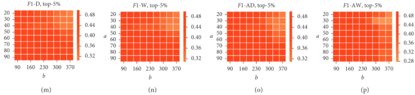
F1-D, top-10% 0.16 0.24 0.32 0.40 0.48 90 80 70 60 50 40 30 20 a 160 230 300 370 90 b (i) F1-W, top-10% 0.16 0.24 0.32 0.40 0.48 90 80 70 60 50 40 30 20 a 160 230 300 370 90 b (j) F1-AD, top-10% 0.16 0.24 0.32 0.40 0.48 90 80 70 60 50 40 30 20 a 160 230 300 370 90 b (k) F1-AW, top-10% 0.16 0.24 0.32 0.40 0.48 90 80 70 60 50 40 30 20 a 160 230 300 370 90 b (l) F1-D, top-5% 0.25 0.30 0.35 0.40 0.45 0.50 90 80 70 60 50 40 30 20 a 160 230 300 370 90 b (m) F1-W, top-5% 0.25 0.30 0.35 0.40 0.45 0.50 90 80 70 60 50 40 30 20 a 160 230 300 370 90 b (n) F1-AD, top-5% 0.25 0.30 0.35 0.40 0.45 0.50 90 80 70 60 50 40 30 20 a 160 230 300 370 90 b (o) F1-AW, top-5% 0.28 0.32 0.36 0.40 0.44 0.48 90 80 70 60 50 40 30 20 a 160 230 300 370 90 b (p)
Figure 10: Influence of a and b for the indicator through accumulated WVG on peak-point prediction performance (F1 score). Warm colors represent high F1 values. Parameter n � 3 when we calculate the indicator with accumulated degree (AD) or accumulated weight (AW) method. 20 30 40 50 60 70 80 90 F1-D, top-20% 0.18 0.24 0.30 0.36 0.42 0.48 a 160 230 300 370 90 b (a) 20 30 40 50 60 70 80 90 F1-W, top-20% 0.24 0.30 0.36 0.42 0.48 a 160 230 300 370 90 b (b) 20 30 40 50 60 70 80 90 F1-AD, top-20% 0.24 0.30 0.36 0.42 0.48 a 160 230 300 370 90 b (c) 20 30 40 50 60 70 80 90 F1-AW, top-20% 0.25 0.30 0.35 0.40 0.45 0.50 a 160 230 300 370 90 b (d) 20 30 40 50 60 70 80 90 F1-D, top-15% 0.24 0.30 0.36 0.42 0.48 a 160 230 300 370 90 b (e) 20 30 40 50 60 70 80 90 F1-W, top-15% 0.32 0.36 0.40 0.44 0.48 a 160 230 300 370 90 b (f ) 20 30 40 50 60 70 80 90 F1-AD, top-15% 0.32 0.36 0.40 0.44 0.48 a 160 230 300 370 90 b (g) 20 30 40 50 60 70 80 90 F1-AW, top-15% 0.32 0.36 0.40 0.44 0.48 a 160 230 300 370 90 b (h) 20 30 40 50 60 70 80 90 F1-D, top-10% 0.24 0.30 0.36 0.42 0.48 a 160 230 300 370 90 b (i) 20 30 40 50 60 70 80 90 F1-W, top-10% 0.18 0.24 0.30 0.36 0.42 0.48 a 160 230 300 370 90 b (j) 20 30 40 50 60 70 80 90 F1-AD, top-10% 0.18 0.24 0.30 0.36 0.42 0.48 a 160 230 300 370 90 b (k) 20 30 40 50 60 70 80 90 F1-AW, top-10% 0.18 0.24 0.30 0.36 0.42 0.48 a 160 230 300 370 90 b (l) Figure 11: Continued.
20 30 40 50 60 70 80 90 a F1-D, top-5% 0.32 0.36 0.40 0.44 0.48 160 230 300 370 90 b (m) 20 30 40 50 60 70 80 90 a F1-W, top-5% 0.32 0.36 0.40 0.44 0.48 160 230 300 370 90 b (n) 20 30 40 50 60 70 80 90 a F1-AD, top-5% 0.32 0.36 0.40 0.44 0.48 160 230 300 370 90 b (o) 20 30 40 50 60 70 80 90 a F1-AW, top-5% 0.28 0.32 0.36 0.40 0.44 0.48 160 230 300 370 90 b (p)
Figure11: Influence of a and b for the indicator through accumulated WVG on trough-point prediction performance. Warm colors represent high F1 value. Parameter n 3 when we calculate the indicator with accumulated degree (AD) or accumulated weight (AW) method. 20 30 40 50 60 70 80 90 a 101 131 181 221 262 350 400 S F1-D, top-20% 0.16 0.24 0.32 0.40 0.48 (a) 20 30 40 50 60 70 80 90 a 101 131 181 221 262 350 400 S F1-W, top-20% 0.16 0.24 0.32 0.40 0.48 (b) 20 30 40 50 60 70 80 90 a 101 131 181 221 262 350 400 S F1-AD, top-20% 0.16 0.24 0.32 0.40 0.48 (c) 20 30 40 50 60 70 80 90 a 101 131 181 221 262 350 400 S F1-AW, top-20% 0.08 0.16 0.24 0.32 0.40 0.48 (d) 20 30 40 50 60 70 80 90 a 101 131 181 221 262 350 400 S 0.25 0.30 0.35 0.40 0.45 0.50 F1-D, top-15% (e) 20 30 40 50 60 70 80 90 a 101 131 181 221 262 350 400 S 0.25 0.30 0.35 0.40 0.45 0.50 F1-W, top-15% (f) 20 30 40 50 60 70 80 90 a 101 131 181 221 262 350 400 S 0.25 0.30 0.35 0.40 0.45 0.50 F1-AD, top-15% (g) 20 30 40 50 60 70 80 90 a 101 131 181 221 262 350 400 S 0.25 0.30 0.35 0.40 0.45 0.50 F1-AW, top-15% (h) 20 30 40 50 60 70 80 90 a 101 131 181 221 262 350 400 S 0.16 0.24 0.32 0.40 0.48 F1-D, top-10% (i) 20 30 40 50 60 70 80 90 a 101 131 181 221 262 350 400 S 0.16 0.24 0.32 0.40 0.48 F1-W, top-10% (j) 20 30 40 50 60 70 80 90 a 101 131 181 221 262 350 400 S 0.16 0.24 0.32 0.40 0.48 F1-AD, top-10% (k) 20 30 40 50 60 70 80 90 a 101 131 181 221 262 350 400 S 0.08 0.16 0.24 0.32 0.40 0.48 F1-AW, top-10% (l) 20 30 40 50 60 70 80 90 a 101 131 181 221 262 350 400 S 0.25 0.30 0.35 0.40 0.45 0.50 F1-D, top-5% (m) 20 30 40 50 60 70 80 90 a 101 131 181 221 262 350 400 S 0.25 0.30 0.35 0.40 0.45 0.50 F1-W, top-5% (n) 20 30 40 50 60 70 80 90 a 101 131 181 221 262 350 400 S 0.25 0.30 0.35 0.40 0.45 0.50 F1-AD, top-5% (o) 20 30 40 50 60 70 80 90 a 101 131 181 221 262 350 400 S 0.25 0.30 0.35 0.40 0.45 0.50 F1-AW, top-5% (p)
Figure12: Influence of a and S for the indicator through accumulated WVG on peak-point prediction performance. Warm colors represent high F1 value. Parameter n 3 when we calculate the indicator with accumulated degree (AD) or accumulated weight (AW) method.
20 30 40 50 60 70 80 90 101 131 181 221 262 350 400 0.24 0.30 0.36 0.42 0.48 a S F1-D, top-20% (a) 101 131 181 221 262 350 400 S 20 30 40 50 60 70 80 90 0.24 0.30 0.36 0.42 0.48 a F1-W, top-20% (b) 20 30 40 50 60 70 80 90 101 131 181 221 262 350 400 0.18 0.24 0.30 0.36 0.42 0.48 a S F1-AD, top-20% (c) 20 30 40 50 60 70 80 90 a 101 131 181 221 262 350 400 0.18 0.24 0.30 0.36 0.42 0.48 S F1-AW, top-20% (d) 20 30 40 50 60 70 80 90 101 131 181 221 262 350 400 0.25 0.30 0.35 0.40 0.45 a S F1-D, top-15% 0.50 (e) 101 131 181 221 262 350 400 S 20 30 40 50 60 70 80 90 0.33 0.36 0.39 0.42 0.45 0.48 a F1-W, top-15% (f) 20 30 40 50 60 70 80 90 101 131 181 221 262 350 400 0.330.36 0.39 0.42 0.45 0.48 a S F1-AD, top-15% (g) 20 30 40 50 60 70 80 90 a 101 131 181 221 262 350 400 0.32 0.36 0.40 0.44 0.48 S F1-AW, top-15% (h) a 101 131 181 221 262 350 400 0.24 0.30 0.36 0.42 0.48 20 30 40 50 60 70 80 90 S F1-D, top-10% (i) 101 131 181 221 262 350 400 S a 0.18 0.24 0.30 0.36 0.42 0.48 20 30 40 50 60 70 80 90 F1-W, top-10% (j) a 101 131 181 221 262 350 400 0.18 0.24 0.30 0.36 0.42 0.48 20 30 40 50 60 70 80 90 S F1-AD, top-10% (k) 20 30 40 50 60 70 80 90 a 101 131 181 221 262 350 400 0.16 0.24 0.32 0.40 0.48 S F1-AW, top-10% (l) 20 30 40 50 60 70 80 90 a 101 131 181 221 262 350 400 S 0.33 0.36 0.39 0.42 0.45 0.48 F1-D, top-5% (m) S 101 131 181 221 262 350 400 20 30 40 50 60 70 80 90 a 0.33 0.36 0.39 0.42 0.45 0.48 F1-W, top-5% (n) S 20 30 40 50 60 70 80 90 a 101 131 181 221 262 350 400 0.36 0.39 0.42 0.45 0.48 F1-AD, top-5% (o) S 20 30 40 50 60 70 80 90 a 101 131 181 221 262 350 400 0.330.36 0.39 0.42 0.45 0.48 F1-AW, top-5% (p)
Figure13: Influence of a and S for the indicator through accumulated WVG on trough-point prediction performance. Warm colors represent high F1 value. Parameter n 3 when we calculate the indicator with accumulated degree (AD) or accumulated weight (AW) method. A re a W AD AW D 0.05 0.10 0.15 0.20 Peak 0.25 0.30 0.35 D W AD AW Trough A re a 0.05 0.10 0.15 0.20 0.25 0.30 0.35
Figure 14: The area under PR curve distribution based on four methods (D, W, AD, and AW) via different a, b, and S parameter combinations. Totally, the AW method performs better than others.
based on the accumulated weight WVG method significantly outperform the others on all 12 datasets.
Among the previous experiments, the parameters are always unchanged (a � 45, b � 131, and S � 262). In order to test the influence of the parameters, we choose different parameter combinations, where a � 20, 30, 40, 50, 60, 70, 80, and 90, b � 90, 125, 160, 195, 230, 265, 300, 335, and 370, and S � 101, 131, 181, 221, 262, 350, and 400, to calculate the
F1 score on the SSE data. Figures 10–13 illustrate the
in-fluence of the combination of a and b and a and S for peak and trough prediction, respectively. And the color repre-sents the F1 score. The influence of the parameter is very significant in the whole range. However, if we focus on the area where a ∈ [40, 90], b ∈ [90, 160], and S ∈ [221, 400], the variance of F1 score is very slight, and the values in this area are also much higher. Additionally, the results based on AW also outperform the other methods in most cases. Similarly with the AUC, we also calculate the area under PR curve as a measure to compare the performance of the four methods, in which a larger area below the curve indicates both greater precision and higher recall. And Figure 14 shows the area distributions. The results show that the proposed methods (AW) perform better than others in most situations.
4. Conclusions
Financial market extremes attract much attention due to their correlation to financial bubbles and crashes. Owing to the extreme complexity of financial markets, phenomeno-logical investigation of stock price data plays a crucial role in gaining a better understanding of financial dynamics. In this work, we aimed to predict the financial extremes from the complex network perspective based on stock indices. The financial extremes are defined as the peak (or trough) points in a long period in the stock market in this work. We proposed indicators according to the accumulated weight of the WVG of the stock price series. Experimental results on 12 major stock indices indicate the strong predictive power of the indicators, which would be an effective indicator for investors to use to adjust their strategies.
Data Availability
The data (12 stock index prices) used in this work can be accessed from the following online address: https://finance. yahoo.com/world-indices.
Conflicts of Interest
The authors declare no conflicts of interest.
Acknowledgments
This study was partially supported by the Zhejiang Pro-vincial Natural Science Foundation of China (grant nos. LR18A050001 and LY18A050004) and Natural Science Foundation of China (grant nos. 61873080 and 61673151).
References
[1] Y. Dong, J.-P. Wang, and T.-Q. Chen, “Price linkage rumors in the stock market and investor risk contagion on bilayer-coupled networks,” Complexity, vol. 2019, Article ID 4727868, 21 pages, 2019.
[2] S. Ali, S. Ahmed, M. Hasan, and R. Ostermark, “Predictability of extreme returns in the Turkish stock market,” Emerging
Markets Finance and Trade, pp. 1–13, 2019.
[3] D. Sornette and W.-X. Zhou, “Predictability of large future changes in major financial indices,” International Journal of
Forecasting, vol. 22, no. 1, pp. 153–168, 2006.
[4] A. Johansen, O. Ledoit, and D. Sornette, “Crashes as critical points,” International Journal of Theoretical and Applied
Fi-nance, vol. 3, no. 2, pp. 219–255, 2000.
[5] Y. Zou, R. V. Donner, N. Marwan, J. F. Donges, and J. Kurths, “Complex network approaches to nonlinear time series analysis,” Physics Reports, vol. 787, pp. 1–97, 2019.
[6] J. Zhang and M. Small, “Complex network from pseudo-periodic time series: topology versus dynamics,” Physical
Review Letters, vol. 96, no. 23, Article ID 238701, 2006.
[7] G. Nicolis, A. G. Cant´u, and C. Nicolis, “Dynamical aspects of interaction networks,” International Journal of Bifurcation
and Chaos, vol. 15, no. 11, pp. 3467–3480, 2005.
[8] L. Lacasa, B. Luque, F. Ballesteros, J. Luque, and J. C. Nuño, “From time series to complex networks: the visibility graph,”
Proceedings of the National Academy of Sciences, vol. 105,
no. 13, pp. 4972–4975, 2008.
[9] X.-K. Xu, J. Zhang, and M. Small, “Superfamily phenomena and motifs of networks induced from time series,” Proceedings
of the National Academy of Sciences of the United States of America, vol. 105, no. 50, pp. 19601–19605, 2008.
[10] C. W. Kulp, J. M. Chobot, H. R. Freitas, and G. D. Sprechini, “Using ordinal partition transition networks to analyze ECG data,” Chaos: An Interdisciplinary Journal of Nonlinear
Sci-ence, vol. 26, no. 7, Article ID 073114, 2016.
[11] M. Wang, H. Xu, L. Tian, and H. Eugene Stanley, “Degree distributions and motif profiles of limited penetrable hori-zontal visibility graphs,” Physica A: Statistical Mechanics and
Its Applications, vol. 509, pp. 620–634, 2018.
[12] X.-H. Ni, Z.-Q. Jiang, and W.-X. Zhou, “Degree distributions of the visibility graphs mapped from fractional Brownian motions and multifractal random walks,” Physics Letters A, vol. 373, no. 42, pp. 3822–3826, 2009.
[13] L. Lacasa, B. Luque, J. Luque, and J. C. Nuño, “The visibility graph: a new method for estimating the Hurst exponent of fractional Brownian motion,” EPL (Europhysics Letters), vol. 86, no. 3, p. 30001, 2009.
[14] L. Lacasa and R. Toral, “Description of stochastic and chaotic series using visibility graphs,” Physical Review E, vol. 82, no. 3, Article ID 036120, 2010.
[15] B. Luque, L. Lacasa, F. Ballesteros, and J. Luque, “Horizontal visibility graphs: exact results for random time series,”
Physical Review E, vol. 80, no. 4, Article ID 046103, 2009.
[16] T.-T. Zhou, N.-D. Jin, and Z.-K. Gao, “Limited penetrable visibility graph for establishing complex network from time series,” Acta Physica Sinica, vol. 61, no. 3, Article ID 030506, 2012.
[17] M. Stephen, C. Gu, and H. Yang, “Visibility graph based time series analysis,” PLoS One, vol. 10, no. 11, Article ID e0143015, 2015.
[18] W. Yan and E. V. Serooskerken, “Forecasting financial ex-tremes: a network degree measure of super-exponential growth,” PLoS One, vol. 10, no. 9, Article ID e0128908, 2015.
[19] C. Liu, W.-X. Zhou, and W.-K. Yuan, “Statistical properties of visibility graph of energy dissipation rates in three-di-mensional fully developed turbulence,” Physica A: Statistical
Mechanics and Its Applications, vol. 389, no. 13, pp. 2675–
2681, 2010.
[20] Y. Zou, M. Small, Z. Liu, and J. Kurths, “Complex network approach to characterize the statistical features of the sunspot series,” New Journal of Physics, vol. 16, no. 1, Article ID 013051, 2014.
[21] H. Sivaraks and C. A. Ratanamahatana, “Robust and accurate anomaly detection in ecg artifacts using time series motif discovery,” Computational and Mathematical Methods in
Medicine, vol. 2015, Article ID 453214, 20 pages, 2015.
[22] R. Zhang, B. Ashuri, and Y. Deng, “A novel method for forecasting time series based on fuzzy logic and visibility graph,” Advances in Data Analysis and Classification, vol. 11, no. 4, pp. 759–783, 2017.
[23] R. Zhang, B. Ashuri, Y. Shyr, and Y. Deng, “Forecasting construction cost index based on visibility graph: a network approach,” Physica A: Statistical Mechanics and Its
Applica-tions, vol. 493, pp. 239–252, 2018.
[24] W.-D. Li and X.-J. Zhao, “Multiscale horizontal-visibility-graph correlation analysis of stock time series,” EPL
(Euro-physics Letters), vol. 122, no. 4, p. 40007, 2018.
[25] M.-C. Qian, Z.-Q. Jiang, and W.-X. Zhou, “Universal and nonuniversal allometric scaling behaviors in the visibility graphs of world stock market indices,” Journal of Physics A, vol. 43, no. 33, Article ID 335002, 2010.
[26] L. Lacasa, V. Nicosia, and V. Latora, “Network structure of multivariate time series,” Scientific Reports, vol. 5, no. 1, p. 15508, 2015.
[27] M. D. Vamvakaris, A. A. Pantelous, and K. M. Zuev, “Time series analysis of S&P 500 index: a horizontal visibility graph approach,” Physica A: Statistical Mechanics and Its
Applica-tions, vol. 497, pp. 41–51, 2018.
[28] E. Zhuang, M. Small, and G. Feng, “Time series analysis of the developed financial markets’ integration using visibility graphs,” Physica A: Statistical Mechanics and Its Applications, vol. 410, pp. 483–495, 2014.
[29] L. L¨u, M. Medo, C. H. Yeung, Y.-C. Zhang, Z.-K. Zhang, and T. Zhou, “Recommender systems,” Physics Reports, vol. 519, no. 1, pp. 1–49, 2012.
[30] L. L¨u and T. Zhou, “Link prediction in complex networks: a survey,” Physica A: Statistical Mechanics and Its Applications, vol. 390, no. 6, pp. 1150–1170, 2011.
Hindawi www.hindawi.com Volume 2018
Mathematics
Journal of Hindawi www.hindawi.com Volume 2018 Mathematical Problems in Engineering Applied Mathematics Hindawi www.hindawi.com Volume 2018Probability and Statistics Hindawi
www.hindawi.com Volume 2018
Hindawi
www.hindawi.com Volume 2018
Mathematical PhysicsAdvances in
Complex Analysis
Journal ofHindawi www.hindawi.com Volume 2018
Optimization
Journal of Hindawi www.hindawi.com Volume 2018 Hindawi www.hindawi.com Volume 2018 Engineering Mathematics International Journal of Hindawi www.hindawi.com Volume 2018 Operations Research Journal of Hindawi www.hindawi.com Volume 2018Function Spaces
Abstract and Applied AnalysisHindawi www.hindawi.com Volume 2018 International Journal of Mathematics and Mathematical Sciences Hindawi www.hindawi.com Volume 2018
Hindawi Publishing Corporation
http://www.hindawi.com Volume 2013 Hindawi www.hindawi.com
World Journal
Volume 2018 Hindawiwww.hindawi.com Volume 2018Volume 2018