A Bayesian technique for conditioning radar precipitation estimates to rain-gauge measurements

HAL Id: hal-00304593

https://hal.archives-ouvertes.fr/hal-00304593

Submitted on 1 Jan 2001

HAL is a multi-disciplinary open access archive for the deposit and dissemination of sci-entific research documents, whether they are pub-lished or not. The documents may come from teaching and research institutions in France or abroad, or from public or private research centers.

L’archive ouverte pluridisciplinaire HAL, est destinée au dépôt et à la diffusion de documents scientifiques de niveau recherche, publiés ou non, émanant des établissements d’enseignement et de recherche français ou étrangers, des laboratoires publics ou privés.

precipitation estimates to rain-gauge measurements

E. Todini

To cite this version:

E. Todini. A Bayesian technique for conditioning radar precipitation estimates to rain-gauge mea-surements. Hydrology and Earth System Sciences Discussions, European Geosciences Union, 2001, 5 (2), pp.187-199. �hal-00304593�

A Bayesian technique for conditioning radar precipitation

estimates to rain-gauge measurements

Ezio Todini

Department of Earth and Geo-Environmental Sciences, University of Bologna, Italy email: todini@geomin.unibo.it

Abstract

The paper introduces a new technique based upon the use of block-Kriging and of Kalman filtering to combine, optimally in a Bayesian sense, areal precipitation fields estimated from meteorological radar to point measurements of precipitation such as are provided by a network of rain-gauges. The theoretical development is followed by a numerical example, in which an error field with a large bias and a noise to signal ratio of 30% is added to a known random field, to demonstrate the potentiality of the proposed algorithm. The results analysed on a sample of 1000 realisations, show that the final estimates are totally unbiased and the noise variance reduced substantially. Moreover, a case study on the upper Reno river in Italy demonstrates the improvements in rainfall spatial distribution obtainable by means of the proposed radar conditioning technique.

Keywords: rainfall, meteorological radar, Bayesian technique, block-Kriging, Kalman filtering

Introduction

At present, there are essentially three basic systems for providing precipitation measurements for use in real-time flood forecasting.

The most common rain sensors for developing operational real-time flood forecasting systems are conventional ground-based telemetering rain-gauges, generally linked to a central station by telephone or radio links (VHF or UHF) or, less frequently, by Meteor-burst equipment or via satellite through Data Collection Platforms (DCPs). Several reasons favour conventional equipment based upon rain-gauges. First, they are the only ones that provide direct— albeit point — measurements of rainfall; second, national services have a tradition of using rain-gauges, so that long historical records are generally available for calibrating rainfall-runoff models; third, in real-time flood forecasting, there is a requirement for other ground-based hydrometeorological measurements, such as water levels in rivers and air temperatures close to the soil, sensors for which may be integrated into the overall data acquisition system so that the cost of additional rain sensors becomes marginal. Finally, in developing countries, training of local personnel and

maintenance is technically and economically more feasible with ground based equipment rather than with weather radars or satellites. The density of raingauge networks depends on several factors (WMO, 1981) and must be determined specifically for each case depending upon the orography and the spatial correlation of observations.

Another precipitation measurement system is the weather radar system, of growing importance in recent decades, particularly since the introduction of dual polarisation systems and Doppler radars. Over one hundred countries now operate 100s of weather radars and development programmes have also been established in several countries (Rosa Dias, 1994). The European Union sponsored COST72 (1985) and COST73 (Collier, 1990) for establishing a weather radar network in participating countries. In the USA, NEXRAD (1984) is a programme to establish a network of 175 S-band Doppler weather radars and, in the UK, the FRONTIERS programme combines radar and METEOSAT images to produce very short precipitation forecasts (Browning, 1979; Browning and Collier, 1982). There are two major benefits in using radars: a finer spatial description of the precipitation field can be obtained and approaching storms can sometimes be observed before they reach the

catchment of interest. A major disadvantage is the need for re-calibration of parameters used for converting reflectivity to rain; this generally requires the installation of a conventional ground-based rain-gauge network.

Until recently, meteorological radar systems have measured only reflectivity (usually indicated as Z). There is no simple correspondence between rain-rate (R) and reflectivity, so hundreds of different Z-R relationships are to be found in the literature. More recently multi-parameter radar rainfall algorithms have been introduced and Gorgucci

et al. (2000) compared their performance.

A common practice in radar hydrology is, therefore, to calibrate the rain-rate derived using either the Z-R or the multi-parameter algorithms by means of rain-gauges: this is generally done using historical data. In real time, a different type of approach is taken, which involves the “adjustment” of the actual radar rain estimates on the basis of the rain-gauge measurements (Atlas et al., 1997).

The third potentially useful measurement system is based upon the analysis of clouds shown by geo-stationary satellite images (Milford and Dugdale, 1989). This approach has been used successfully in tropical areas and, in particular, for the development of the Nile Flood Early Warning System (Grijsen et al., 1992), but has not yet reached the quality required to implement operational flood forecasting systems on small or medium size catchments in sub-tropical areas.

Several techniques using meteorological radar/rain-gauge adjustment have been developed (also usable for satellite estimates): the spatial adjustment method, based upon an empirical negative exponential weighting, in its original formulation (Barnes, 1964; Brandes, 1975) involves the generation of a matrix of weights, or in slightly modified versions as proposed by Moore et al. (1989), Uijlenhoet et

al. (1994); the domain adjustment technique (Collier et al,

1983); the mean-field bias adjustment (Ahnert et al., 1983; Lin and Krajewski, 1989); the radar-gauge coKriging (Creutin et al., 1986; Krajewski, 1987, Seo et al., 1990a,b). Unfortunately, the coKriging technique is applicable only if one can actually compute the right-hand sides of a system of linear equations in terms of the covariances between true value of precipitation and both the gauge measurements and the radar estimates. This is obviously impossible because the true precipitation values are unknown. Krajewski (1987) approximated it on the basis of the radar covariance matrix but this is unsatisfactory since, unless the right-hand sides are known, the level of approximation of the final solution may become very large. A second problem relates to the co-Kriging constraints; in practice these require that, at each time-step, the total volume of rain must equal that estimated by the gauges, while the constraints should be set in a less rigid form on the expected values in time.

More recently, attention has been focused on multi-sensor merging using physically-based models (Lee and Georgakakos, 1990; Georgakakos and Krajewski, 1991; Seo and Smith, 1991a,b; French and Krajewski, 1994; French

et al., 1994).

While their conclusions on the effect of radar and rain-gauge combination are generally positive in terms of bias reduction (Borga et al., 2000), they seem rather negative in terms of reduction of variance. In the case of uncertain covariance, Bayesian techniques have been used in Kriging for parameter estimation and the assessment of the uncertainty induced on the Kriging spatial functions (Kitanidis, 1986; Omre and Halvorsen, 1989; Le and Zidek, 1992; Handcock and Stein, 1993). A Bayesian formulation was used by Seo and Smith (1991a,b) to improve radar precipitation estimates by raingauge measurements, limiting their approach to the reduction of bias. In contrast, this paper introduces an original Bayesian combination technique that aims not only at eliminating the bias of meteorological radar precipitation estimates but also at producing minimum variance precipitation estimates on pixels of variable sizes ranging, for instance, from 1×1 to 10×10 km2_.

The first problem to be solved is that point measurements, such as are produced by rain-gauges, based upon a funnel of 1000 cm2 _{catch area, cannot be compared directly to the}

average values of radar estimates over pixels of 1×1 km2 _or

even larger. Hence, it is proposed to use block-Kriging to estimate the average field over the radar pixels and its variance from the point raingauge measurements.

The two estimates obtained from radar and rain-gauges are now comparable and, since it is reasonable to assume that they are independent estimates of the same unknown quantity, the effects of the two different estimation errors can be separated from their differences (Pereira Filho and Crawford, 1997).

Assuming that the rain-gauge estimates are unbiased, once the estimation error statistics have been determined, a Kalman Filter approach is taken to find the a posteriori estimates by combining the a priori estimates provided by the radar with the block-Kriged measurements provided by the gauges in a Bayesian framework.

Derivation of the proposed

methodology

Given a random field y of precipitation on a lattice, which_tR

can be produced using radar (in real or in a log-transformed space), the problem of conditioning it to a set of point measurements, such as for instance the ones produced by rain-gauges, can be tackled as follows.

The first problem to be solved is that point measurements, such as those produced by rain-gauges that in the best case

are based upon a funnel of 1000 cm2 _{catch area, cannot be}

compared with average values of radar estimates over pixels

of 1 km2 _{or larger sizes. This inconsistency can be found}

for instance in Pereira Filho and Crawford’s approach (1997), which uses the direct point differences between rain-gauges and radar estimates in a correction algorithm. In addition, the nature of their errors is quite different and complementary: rain-gauge measurements tend to be more accurate at a point while their spatial significance decays with distance and, hence, with area; in contrast, radar provides a better spatial (although biased) representation but a much poorer quantitative estimate.

To combine the two sets of data consistently, the first step is to regionalise the point rain-gauge measurements on a lattice made of pixels, on which the radar estimates are given, by means of block-Kriging and to estimate on this lattice the error statistics of the block-Kriged variables.

Rain-gauges, and in particular the most commonly used tipping-bucket rain-gauges, are relatively accurate instruments subject only to the so-called “volumetric” or “undercatchment” error, i.e. the fact that, at higher rain intensities, part of the water is not “weighed” by the tipping-bucket mechanism, thus violating the usual assumption that the volume of water needed to cause the bucket to tip is independent of the rainfall intensity. Nevertheless, Humphrey et al. (1997) and Lombardo and Staggi (1998), showed that this error is essentially a bias, with a small dispersion around it, that can be corrected, effectively, using the following (or similar calibration curves), with:

β

α IG

I = ⋅ (1)

where:

I is the actual rain intensity;

G

I the rain-gauge measured intensity or the tipping rate

(Niemczynowicz, 1986); β

α, rain-gauge specific calibration parameters whose

values are generally provided by the manufacturer and determined using special equipment such as the one described by Humphrey et al. (1997).

Other sources of error are due to evaporation that affects tipping bucket type gauges only at values smaller than their sensitivity, generally 0.2 mm using a standard WMO

1000 cm2 _{funnel, (WMO, 1981), while errors due to wind}

effect can be reduced, but not totally eliminated, either by protective screens around the rain-gauge or by placing the rain-gauge at ground level, as proposed by the Institute of Hydrology, Wallingford. UK.

If one denotes the vector of n raingauge measurements at

time t , as G t

x , a Kriging estimate of ytG on all the pixels

of the lattice can be produced using the expression:

G t G

t x

y =Λ (2)

where Λ, the [m, n] matrix of weights, is obtained as:

[

] [

]

1 0 −           = M L L L M M M T lb u u u Γ Γ µ Λ (3)

in which, with the usual Kriging notation Γ is the [n,n]

semi-variogram matrix among the n measurement points (the location of the rain-gauges), Γlb represents the [m, n]

semi-variogram matrix between the number of lattice squares m and the number of measured points n, u is an [m] vector of ones and µ an [m] vector of Lagrange multipliers. From the above discussion on error sources, the rain-gauge point measurements are considered unbiased, in that the bias can be corrected dynamically using Eqn. (1), while the measurement uncertainty can be accounted for, without formally changing Eqn. (3), by modifying the definition of the semi-variogram matrix, Γ , slightly, by subtracting from its principal diagonal the variance of the measurement errors, under the reasonable assumption of independence among errors affecting the different gauges (de Marsily, 1986).

Initially,Γ can be estimated from historical records on the assumption of second order stationarity in time of the rainfall field, for a given weather type, and updated as a function of the latest observations. Bayesian techniques, such as the one proposed by Omre and Halvorsen (1989) and Le and Zidek (1992) will be investigated for parameter estimation and parameter update.

Pereira Filho and Crawford (1997) pointed out that it is reasonable to assume that the two measurement systems, namely radar and rain-gauges, provide independent measures of the same unknown quantity. Therefore, their difference G t R t t = y −y ε (4)

which, by adding and subtracting the true but unknown random field yt, can also be written as:

(

) (

t

)

G t t R t t = y −y − y −y ε (5)

and can be used to assess the stochastic properties of the errors of estimate of the random field produced by the radar, by estimating its sample mean and its sample covariance. The statistical properties of εt can be expressed as:

{ }

{

} {

}

G t R t t t G t t R t t E y y E y y Eε =µ_ε = − − − =µ_ε −µ_ε (6)

(

)(

)

{

}

[

(

)

]

[

(

)

]

(

)

[

]

[

(

)

]

G t R t G t G t R t R t t t t V V y y y y E y y y y E V E T t G t t G t T t R t t R t T t t ε ε ε ε ε ε ε ε ε µ µ µ µ µ ε µ ε + =     _{− − − −} +     _{− − − −} = = − − (7) t z , to give: G t G t t y x z = =Λ (12)

Equation (12) can also be written in terms of the true but unknown field yt to give:

(

t

)

G t t G t y y y y = + − (13)

or, using the standard Kalman filter notation:

t t t t H y

z = +η ₍₁₄₎

After substituting in Eqn. (13)

t G t t = y −y η (15) and setting I Ht = (16)

Equation (14) can now be considered as the measurement equation of a classical Kalman filter (Kalman, 1960; Kalman and Bucy, 1961) in which:

{ }

= =

{

−

}

= G =0 t t t G t t E y y Eη µ_η µ_ε (17)

{ }

[

(

)

]

[

(

)

]

[

]

ll T T T T t G t t G t T t t u u V y y y y E V E G t G t G t t Γ µ Λ Γ µ Λ µ µ η η η _{ε ε ε} −                     = =     _{− − − −} = = L M L L L M M 0 (18)

At this point, by taking

R t R t t y y′= −µ_ε (19)

as the a priori estimate of the state and

R t

V

P_t′= _ε (20)

as the a priori estimate of its covariance matrix, it is possible where the expected value (the bias) and the covariance

matrix of εt are given as a function of the expected values

and the covariances of εtR and G t

ε , namely the radar pixel

average estimation error and the block-Kriged rain-gauge measurement error respectively. Bearing in mind that Kriging (as well as block-Kriging) is unbiased and allows for the estimation of the covariance matrix of the estimation errors, the following result may be verified easily: ₌₀ G t ε µ (8)

[

]

ll T T T u u V G t Γ µ Λ Γ µ Λ ε −                     = L M L L L M M 0 (9)

where Γ_ll is the [m, m] semi-variogram matrix among all

the reconstructed lattice squares. Thus by substituting Eqns. (8) and (9) into Eqns. (6) and (7), it is possible to estimate

and as: t R t ε ε µ µ = (10)

[

]

            −                     − = ll T T T u u V V t R t Γ µ Λ Γ µ Λ ε ε L M L L L M M 0 (11)

where µε_t and V_εt can be estimated, from the time series of Eqn. (4), using a number of historical rainfall events. Additional research is needed for assessing the most appropriate technique for estimating

t

ε

µ and V_εt: at the present time the estimation is based upon the assumption, for a given weather type, of second order stationarity in time of the differences εtgiven by Eqn. (4), while it is the

intention of the writer to implement a Bayesian updating scheme for real time applications.

To combine the two sets of measurements (namely the block-Kriged point rain-gauge measurements and the radar lattice estimates) in a Bayesian way, one of the two random

fields (in this paper, the one produced by the radar R

t y ) is

taken as the a priori estimate and the other one (in this paper,

that produced by the radar G

t

y ), as the measurement vector R

t

ε

to compute the innovation νt as: R t R t G t t t t t z H y Λx y µ_ε ν = − ′= − − (21)

and the Kalman gain

t K as:

(

_′+

)

−1₌

(

₊

)

−1₌ −1 ′ = t R t G t R t R t t V V V V V V P P K_{t t t η ε ε ε ε ε} (22)

Finally, the Kalman Filter equations allow the a posteriori estimate to be found by combining the a priori estimate and the measurements in a Bayesian framework to give:

(23) R t t R t R t V V V V P H K P P_t′′= _t′− _{t t t}′= _ε − _{ε ε}−1 _ε (24)

where yt′′ is the a posteriori estimate of the random field

over the lattice and P_t′′ its error of estimate covariance matrix. The solution proposed by Eqn. (23) is not limited to a radar bias correction, as in Ahnert et al., 1986; on the contrary, the proposed technique offers a multivariate Bayesian combination of radar estimates and raingauge measurements on the basis of the local relative uncertainty. Finally, the developed Kalman filter is based upon a “static” formulation in which the time evolution of the measurement error structure is not taken into account. Further improvements to the proposed methodology, requiring real-time updates of the means and covariance matrices as a function of their time evolution, will be tested in the future.

A numerical example

Because the true rainfall field is unknown in real-world applications, it was felt necessary to demonstrate the effectiveness of the proposed methodology in terms of the

a posteriori estimates convergence towards the true, but

supposed unknown values, by means of a numerical example.

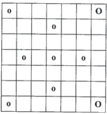
In the proposed example, the radar measurements are assumed to be available on a 7×7 lattice with sides of 1000 m, while nine rain-gauges are assumed to be set in the centres of the lattice cells, as in Fig. 1.

A Gaussian random field yt, taken as the true field, is

then generated jointly on the lattice and on the measurement points, for 1000 time-steps, with the following covariance

= −_p+  −e−h a_ 2 1 2 _ω σ and parameters as in Table 1.

Table 1. Random field parameters

( )

µ

Mean Variance

( )

σ2 Nugget

( )

p Sill

( )

ω Range

( )

a

0 10,000 0 10,000 107

This generation involved the computation of the following covariance matrix:           = Γ Γ Γ Γ M L L L M bl lb ll T BB (25)

and the derivation of its square root B by the eigenvalue-eigenvector decomposition and the generation of the process vector at each time interval, namely:

t b l t b l B y y           =           δ δ L L (26)

where δ_l,δ_b are 49+9 NIP(0,1) variables.

In the example, the rain-gauge point measurements are considered unaffected by measurement errors, while the radar estimates are considered biased and affected by noise. Therefore, 1000 time realisations of a Gaussian random noise were generated with the parameters given in Table 2.

Table 2. Random noise field parameters

( )

µ

Mean Variance

( )

σ2 Nugget

( )

p Sill

( )

ω Range

( )

a

40 3,000 0 3,000 106

The noise was then added to the “true” value

[ ]

yl t to give

the noise corrupted observations y similar to the ones onetR

could expect from a radar. In practice, the error represents a very large bias and a variance of the order of 30% of the signal. The data used for the analysis were then the 1000 sets of 49 noise corrupted “radar” estimates on the lattice

(

R

)

t t R t R t R t G t R t t t t t y K y V V x y y′′= ′+ ν = −µ_ε + _{ε ε} −1Λ − −µ_ε

Fig. 1. The lattice and the location of the gauges

and the corresponding 1000 sets of nine perfect point “raingauge” measures.

To show the efficiency of the proposed procedure, it was applied on the assumption that the random field parameters were known, so that no estimation error was involved in the process.

Through application of the Kalman Filter Eqn. (23), 1000 sets of 49 a posteriori estimates were obtained. The “true” field was then subtracted both from the a priori as well as from the a posteriori estimates and the statistics were computed for all the lattice cells.

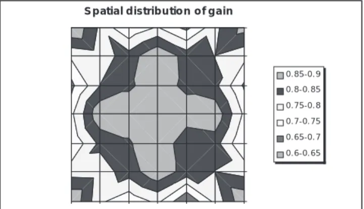
Although dealing with purely Gaussian fields where the methodology is by definition “optimal”, the results are nonetheless impressive. The bias has been totally eliminated over the entire lattice (Fig. 2), while Fig. 3 shows that the standard deviation of errors has been more or less halved. Figure 4 shows the variance gain, namely the percentage reduction in variance, which varies between 90% and 65% as a function of the distance from the rain-gauges and from the centre as is shown in Fig. 5 where the gain is plotted for the different cells.

The proposed method performs far better than the empirical negative exponential weighting used by Brandes (1975), for which no bias elimination and no minimum variance weighting parameter estimation is applied, leaving the parameter choice to subjective judgement.

Finally, it is not expected that the estimation of the Kriging parameters will modify strongly the results obtained, given their small influence on the estimation of the covariance matrix, for which a decent approximation produces good results.

The case study

To analyse the performance of the proposed methodology on real-world data, a case study was set up on the upper Reno river close to Casalecchio, near Bologna (Italy), where several rain-gauges and a meteorological radar are available.

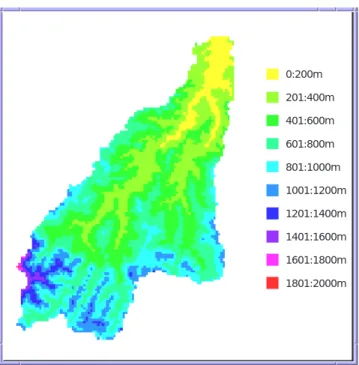
The river catchment has a surface area of 1051 km2 _and

ranges in elevation from 0 to 2000 m, as shown by the Digital Terrain Model in Fig. 6. Combined with the prevailing extension of clayey and marly soils, with a few alluvial deposits in its terminal section, the catchment gives rise to flood waves that can reach 1900 m3_s-1_.

-1 0 0 1 0 2 0 3 0 4 0 5 0 1 5 9 13 1 7 21 25 2 9 33 37 4 1 4 5 49 C e l l n u m b e r M ean A p riori m e an A p os t erio ri m ean 0 10 20 30 40 50 60 1 4 7 10 13 16 19 22 2 5 28 31 3 4 37 40 43 46 4 9 C e l l n u m b e r S tan d a r d D e vi a ti o n A prio ri S t d. A pos te riori S t d.

Fig.2. Bias reduction in the 49 lattice cells

0 % 20 % 40 % 60 % 80 % 100 % 1 4 7 10 1 3 1 6 19 22 25 28 31 3 4 3 7 4 0 43 46 49 C e l l n um b e r P e rc e n ta g e v a ri a nc e re du c ti o n G ain

Fig. 3. Standard deviation reduction in the 49 lattice cells

S p atia l d istrib u tio n o f g a in

0. 85-0. 9 0. 8-0. 85 0. 75-0. 8 0. 7-0. 75 0. 65-0. 7 0. 6-0. 65

Fig. 4. Percentage variance reduction (gain) for the 49 cells

AVAILABLE DATA

The Regional Meteorological Service provides hourly maps of rainfall estimated by a C-band Doppler radar is located about 30 km north-east of Casalecchio, in the Po Valley; its main characteristics are given in Table 3. A double polarisation radar like the one available, emits electromagnetic impulses polarised in orthogonal directions,

measuring the differential reflectivity Z_DR, that is the

difference between reflectivity values in the two different polarisation (Z_H, Z_V horizontal and vertical) directions:

    = V H Z Z 10log Z_DR (27)

Fig. 6. The Digital Terrain Model (DTM) of the upper Reno River

Radar data are obtained from reflectivity volumetric measures with 250 m range resolution for several elevations (0,5°, 1,4°, 2,3°) and azimuths. The composite reflectivity PPI (Plan Position Indicator) maps are constructed by

averaging spatially over cells of 1×1 km2 _{and, depending}

on the orography, at any azimuth and range the first PPI not

Table 3. The meteorological radar characteristics

Managing agency Regione Emilia-Romagna

Site (denomination, lat., long.) S.Pietro Capofiume 44°39’, -0°50’

Height a.s.l. 11 m

Capability Doppler Double Polarisation

Band C Wavelength 5.5 cm Processing digital Antenna Beam width 0.9 Polarisation horizontal Gain >45 dB

Scanning method volumetric, sectorial

Transmitter/Receiver

Frequency 5450-5650 MHz

Type klystron

Pulse length and ass. PRF 0.5, 1.5, 3.0 ms –1200, 600, 300 Hz

Receiver type Log and Lin

Band Log. dynamic range 80 dB

Band Lin. dynamic range from 30 dB to 90 dB with I.A.G.C.

RSP/RDP

Range bin 125, 250, 500 m - 1 km

Covering Range 125, 250 km

Possible resolutions 125 m at 125 km, 250 m at 250 km

Range

Possible diff. op. outputs CAPPI Z, Z_DR, v, s_v, HVMI

Scan strategy every 5 min. vol. acquisition

Max height of RDP outputs 16 km

0:200m 201:400m 401:600m 601:800m 801:1000m 1001:1200m 1201:1400m 1401:1600m 1601:1800m 1801:2000m

considerably affected by the ground echoes (clutter) is retained. Furthermore, an algorithm able to eliminate anomalous propagation echoes is also running at the Regional Meteorological Service.

The 1×1 km2 _{maps are collected every 15 minutes and}

converted into rainfall intensity by means of the classical Marshall and Palmer relationship and the rainfall intensities are then averaged to obtain hourly cumulative rainfall data. Several recording rain-gauges are also available in the upper Reno river catchment. Table 4 provides a list of the 26 gauges used in the case study together with their geographical position and the elevation in metres a.s.l.

The case study refers to the eight days from 4–11 November, 1994. This event was chosen because of anomalous radar precipitation estimates. This anomaly can be detected from Fig. 7, where the discharges measured at Casalecchio (thick black line) are compared to those estimated by a rainfall-runoff model using alternatively: (1) the precipitation obtained by Kriging the point rain-gauge measures (thin grey line) or (2) the radar estimated rainfall (thick grey line), as the input to the model. While the first part of the flood event is reproduced well using both areal rainfall estimates produced by the rain-gauges and the radar, the second part is reproduced only by the gauges, while the radar underestimate the rain intensity over the catchment. The cause of this anomaly can neither be interpreted as a lack of radar calibration, because radar performed quite well during the first portion of the event nor as a consequence of radar failures (Fig. 8 shows the period of radar failures), which happened on 46 of the 192 hours, luckily during either dry or very light rain spells.

In summary, the following data were available for the case study:

(1) 146 hours of radar precipitation estimates at 1084 pixels of 1×1 km2_;

(2) The geographical co-ordinates of the 1084 pixels; (3) 192 hours of rain-gauge precipitation measurements at

26 locations;

(4) The geographical co-ordinates of the 26 rain-gauge locations;

ESTIMATION OF SEMI-VARIOGRAM AND RELEVANT PARAMETERS

Following the procedure proposed, the first step is to apply block-Kriging to the point rain-gauge measurements, which requires the estimation of the semi-variogram, and relevant parameters, from the 26 rain-gauge measurements.

Several hours of rainfall measurements were available, so the semi-variogram was not estimated by using the classical Kriging approach which takes into consideration a unique set of measures in time: rather, the semi-variogram was derived from an estimate of the covariance matrix, which was based on all the available data in space and time. Moreover, given that several time intervals were dry, not all the 192 available measurement hours were used to estimate the spatial correlation; hourly measurements showing no rain in more than five gauges were rejected: this reduced the 192 hours of measurement to only 47.

Once the covariance matrix is available, the semi-variogram value can be computed from its definition as:

Table 4. List of rain gauge stations in the upper Reno river

basin

n Gauging station LAT.(1) _LON.(2) _Elevation

(m a.s.l.) 1 Piastre 44°03' 1°31' 741 2 Maresca 44°04' 1°36' 1,043 3 Pracchia 44°03' 1°32' 627 4 Orsigna 44°05' 1°34' 806 5 Monte Pidocchina 44°04' 1°31' 1,100 6 Diga di Pavana 44°07' 1°27' 480 7 Porretta Terme 44°09' 1°28' 349

8 Monteacuto delle Alpi 44°08' 1°34' 915

9 Lizzano in Belvedere 44°09' 1°33' 640 10 Bombiana 44°13' 1°29' 804 11 Acquerino 44°00' 1°26' 890 12 Treppio 44°05' 1°25' 710 13 Diga di Suviana 44°08' 1°25' 500 14 Riola di Vergato 44°13' 1°23' 240 15 Vergato 44°17' 1°20' 195 16 Cottede 44°07' 1°16' 850

17 Diga del Brasimone 44°07' 1°20' 830

18 Monteacuto Vallese 44°14' 1°15' 747

19 Monzuno 44°16' 1°11' 620

20 Sasso Marconi 44°23' 1°13' 130

21 Montepastore 44°22' 1°20' 596

22 Monte San Pietro 44°22' 1°05’ 317

23 Bologna San Luca 44°29' 1°09' 286

24 Monghidoro 44°13' 1°08' 841

25 Pianoro 44°22' 1°06' 187

26 Traversa 44°06' 1°10' 871

(1)_{1' in latitude is equal to 1850 m.}

(2)_{The longitude refers to the Rome Meridian (Monte}

Mario). The longitude of Monte Mario in relation to Greenwich is 12°27’08'’

Reno River September '94 Radar-Kriging discharges 0 50 100 150 200 250 300 350 400 1 7 13 19 25 31 37 43 49 55 61 67 73 79 85 91 97 _{103 109 115 121 127 133 139 145 151 157 163 169 175 181 187} hours discharges (m3/s) Observed Radar Kriging 0 1 2 1 25 49 73 97 121 145 169 193 Hours

Fig. 7. Discharges measured at Casalecchio (thick black line) and estimated using the Kriged point rain-gauge measures (thin grey line) or

the radar estimated rainfall (thick grey line)

Fig. 8. Periods of available (0) and missing (1) radar data

( )

hi,j =

[

Cov

( )

i,i +Cov

( )

j,j −2⋅Cov

( )

i,j

]

2

1

γ (28)

wherehi,j is the distance between the two rain-gauges i and j.

The semi-variogram model and its parameter values can then be estimated in the classical way by dividing the maximum distance among the rain-gauges in classes (in this case 5000 m distance classes were used), by computing the average value per class and by fitting the different models as a function of their parameter values.

In the proposed case, the best results were obtained using the Gaussian semi-variogram, given in Eqn. (29) as a function of its three parameters, p the nugget, ω the sill and a the range:

( )

( ) _   − + = − 2 1 e ha p h ω γ (29)

Table 5. Gaussian semi-variogram parameter

value estimates

( )

p

Nugget Sill

( )

ω Range

( )

a

2.66 1148 951048 0 2 4 6 8 10 0 10000 20000 30000 40000 50000 60000 D is tance [m] S e m i-v a ri o gr am Sample Gaussian

Fig. 9. Gaussian semi-variogram compared to sample estimates

limits

σ

2

±

The parameter values obtained are given in Table 5, while Fig. 9 compares the sample estimates, plus or minus two sigma limits, and the estimated Gaussian semi-variogram.

ESTIMATION OF BLOCK SEMI-VARIOGRAMS

The application of the proposed methodology, based upon the block-Kriging and the Kalman Filter, requires the estimation of the following matrices which contain the

semi-variogram values computed among gauges (Γ ), among

gauges and radar pixels(Γlb), among radar pixels (Γ_ll).

In the proposed case study, the matrix Γ is the

symmetrical [n+1, n+1] matrix, with n=26 the number of gauges, defined as:

                    = 0 1 1 1 1 1 0 1 1 0 1 0 1 0 3 2 1 3 32 31 2 23 21 1 13 12 ... ... ... ... ... ... ... ... ... ... n n n n n n γ γ γ γ γ γ γ γ γ γ γ γ Γ (30)

where γi,j =γ

( )

hi,j is computed using Eqn. (29).

The matrix Γ_lb is the [m, n+1] matrix, with m=1084 the number of radar pixels, defined as:

                    = 1 1 1 1 2 1 3 32 31 2 22 21 1 12 11 mn m m n n n lb ... ... ... ... ... ... ... ... ... ... ... ... ... ... γ γ γ γ γ γ γ γ γ γ γ γ Γ (31)

where γi,j is estimated, according to Eqn. (32) as the

average over pixel j of the semi-variogram from point i:

(

) (

)

∫ ∫

∫ ∫

 − + −  = j j j j x y x y i i j , i d d d d y x η ξ η ξ η ξ γ γ 2 2 (32)

The matrix Γ_ll is the symmetrical [m, m] matrix, defined

as:                 = mm m m m m m ll ... ... ... ... ... ... ... ... γ γ γ γ γ γ γ γ γ γ γ γ Γ 2 1 3 32 31 2 22 21 1 12 11 (33) where

(

) (

)

∫ ∫ ∫ ∫

∫ ∫ ∫ ∫

 − + −  = i i j j i i j j x y x y x y x y j , i d d d d d d d d ζ χ η ξ ζ χ η ξ η ζ ξ χ γ γ 2 2 (34)

The integrals appearing in Eqns. (32) and (34) can be computed easily for the Gaussian model since an analytical expression can be derived for squared or rectangular pixels, while numerical estimates must be used for most of the other semi-variogram types and integration domains.

The matrices of Eqns. (30), (31) and (32) are exclusively a function of the semi-variogram as well as of the co-ordinates of the rain-gauges and of the radar pixels; therefore, they are kept unchanged as a function of rainfall data. This implies the assumption of weak stationarity in time for the first and second moments of the rainfall process. When a unique weather type is driving the rainfall event, as in the present case study, this hypothesis seems reasonable. Nevertheless, further investigation must be carried out to assess the effect of changes in the spatial covariance (as well as in the semi-variogram) structure as a function of changed weather type conditions, which would recommend the use of different estimates according to the specified weather type.

APPLICATION RESULTS

Once the matrices were estimated, the block-Kriging Bayesian correction technique was applied to the 146 available contemporary rain-gauge and radar measurements. As opposed to the earlier numerical example, in the real-world case study, the true value of the precipitation over each pixel is unknown, which means that the actual variance reduction cannot be estimated. Nevertheless, it is possible to evaluate the reduction of bias and of time variance between ytG, the block-Kriged rainfall, derived from the

rain-gauges, and y_t′′, the a posteriori estimate, by computing

the difference

(

G _t

)

t y

y − ′′ and by estimating its expected value and covariance matrix. Given the large size of the matrices [1084×1084] and vectors [1084] involved, an overall measure of results will be given by averaging in space over the 1084 pixels the resulting performances.

Table 6. Bias and variance reduction

Variable A priori

(

t

)

G t y y − ′ A posteriori

(

y_tG−y_t′′

)

Bias 0.34 0.07 Variance 11.29 1.87

While, on the assumption that the block-Kriging is unbiased, the bias reduction is actually representative of the improvements, the variance reduction must be considered cautiously. As discussed earlier, G

t

y and y′t can be assumed

independent but this is not true for G t

y and yt′′ since the a posteriori estimate incorporates the information brought by

the measurement. Therefore, taking into account the fact that the two series are not independent, part of the large reduction obtained in the overall variance is due to the increased correlation between the time pattern of the two time series, which is itself a beneficial property.

This was not so in the previous numerical simulation

example, where yt the “true” value of precipitation was

known and used to measure the reduction in variance from

(

yt yt

)

Var ′− to Var

(

y_t′′−y_t

)

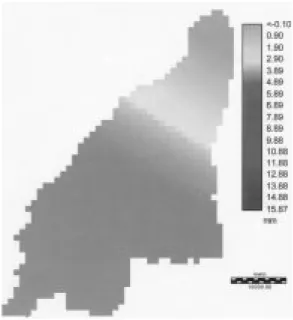
, which is why it was felt essential for the completeness of this research.

Fig. 10. Block Kriged rain-gauges

Fig. 11. Radar rain estimates

Fig. 12. Bayesan combination

In a more qualitative manner, the results of the case study can be discussed by looking at Figs. 10, 11 and 12 which show the effect of the proposed method during the anomalous behaviour of the radar. The figures refer to the 160th hour. Figure 10 shows the smoothed surface, produced by block-Kriging, of the rainfall intensities increasing from the northern lower edge to the upstream southern mountain part of the catchment. Figure 11 shows what was estimated on the basis of the radar data: there was a heavy rainstorm in the upper part of the catchment, with practically no rain anywhere else. Figure 12, the Bayesian combination, extends the amount of rainfall estimated by the radar to the other portions of the catchment, while preserving the spatial variability. This does not mean that this is the true rainfall: this is only a more likely estimate in which the uncertainty in the different measurement methods has been reduced successfully.

Conclusions and further work

The new block-Kriging-Bayesian technique for combining weather radar based rainfall estimates with rain-gauge measurements is open to a wide range of possible applications. The technique is needed particularly for real-time flood forecasting applications where the reliability and the reduction of uncertainty are the major requirements. To this end, it is expected that the proposed methodology will increase the credibility of the radar based rainfall estimates. The test on numerical data has demonstrated the efficiency of the technique and application to real-world data has giver qualitative confirmation of the improvements that can be obtained by its application.

block-Kriging-Bayesian approach, further tests and analyses will be performed within the frame of MUSIC. These will deal with the comparison of the proposed technique with the co-Kriging radar-rainfall approach of Krajewski (1987); the analysis of the relevance of the rain gauge measurement errors; the assessment of the effects of time variations in the rainfall spatial co-variance structure as a function of the different weather types and the possibility of a Bayesian update for their estimates.

Nonetheless, extensive application of the technique is anticipated within the frame of a recently approved EU-funded project MUSIC (Multi Sensor precipitation measurements Integration, Calibration and flood forecasting) where, in addition, a combination of three different measurement systems (weather radar, satellite and rain-gauges) will be tested for the benefit of all possible sources of independent information.

References

Ahnert, P.R., Hudlow, M.D., Greene, D.R. and Johnson, E.R., 1983. Proposed on site precipitation processing system for NEXRAD. Preprint, 21st Conference on Radar Meteorology, Edmonton, Alberta, Canada.

Ahnert, P.R., Krajewski, W.F. and Johnson, E.R., 1986. Kalman filter estimation of radar-rainfall field bias, Preprint, 23rd

Conference on Radar Meteorology, American Meteorol. Soc.,

JP 33-37.

Atlas, D., Ryzhkov, A. and Zrnic, D., 1997. Polarimetrically tuned Z-R relations and comparison of radar rainfall methods. In:

Weather Radar Technology for Water Resources Management,

B. Braga Jr. and O. Massambani (Eds.). UNESCO Press, Paris, France, 3–67.

Barnes, E.A., 1964. A technique for maximising details in numerical weather map analysis. J. Appl. Meteorol., 3, 396– 409.

Borga, M., Anagnostou, E.N. and Frank, E., 2000. On the use of real-time radar rainfall estimates for flood predictions in mountainous basins. J. Geophys. Res. 105, 2269–2280. Brandes, E.A., 1975. Optimizing Rainfall Estimates with the Aid

of Radar. J. Appl. Meteorol., 14, 1339–1345.

Browning, K.A., 1979. The FRONTIERS plan: a strategy for using radar and satellite imagery for short range precipitation forecasting. Meteorol. Mag., 108, 161–184.

Browning, K.A. and Collier, C.G., 1982. An integrated radar-satellite nowcasting system in the UK. In: Nowcasting, Browning K.A. (Ed.). Academic Press, London, 47–61. Collier, C.G., Larke, P.R. and May, B.R., 1983. A weather radar

correction procedure for real-time estimation of surface rainfall.

Quart. J. Roy. Meteorol. Soc., 109, 589–608.

Collier, C.G., 1990. COST 73: The development of a weather radar network in Western Europe. In. Weather Radar Networking

Seminar on COST Project 73, C.G.Collier and M.Chapuis

(Eds.). Kluwer Academic Publishers, Netherlands, EUR 12414 EN - FR.

COST Project 72, 1985. European Commission Report EUR 10353 EN - FR.

Creutin, J.D., Delrieu, G. and Lebel, T., 1986. Rain measurement by raingauge-radar combination: a geostatistical approach. J.

Appl. Atmos. Ocean. Technol., 5, 102–115.

de Marsily, G., 1986. Quantitative Hydrogeology, Academic Press. French, M.N. and Krajewski, W.F., 1994. A model for real time rainfall forecasting using remote sensing, 1, Formulation. Water

Resour. Res., 30, 1075–1083.

French, M.N., Andrieu, H. and Krajewski, W.F., 1994. A model for real time rainfall forecasting using remote sensing, 2, Case Studies. Water Resour. Res., 30, 1085–1094.

Georgakakos, K.P. and Krajewski, W.F., 1991. Worth of radar data in the real time prediction of mean areal rainfall by non-advective physically based models. Water Resour. Res., 27, 185– 197.

Gorgucci, E., Scarchilli, G. and Chandrasekar, V., 2000. Sensitivity of multiparameter radar rainfall algorithms. J. Geophys. Res. 105, 2215–2223.

Grijsen, J.G., Snoeker, X.C., Vermeulen, C.J.M., Mohamed El Amin Moh. Nur and Yasir Abbas Mohamed, 1992. An information system for flood early warning. In: Floods and

Flood Management, A.J.Saul (Ed.). Kluwer Academic

Publishers, 263–289.

Handcock, M.S. and Stein, M.L., 1993. A Bayesian analysis of Kriging. Technometrics, 35, 403–410.

Humphrey, M.D., Istok, J.D., Lee, J.Y., Hevesi, J.A. and Flint, A., 1997. A new method for automated dynamic calibration of tipping-bucket rain gauges. J. Atmos. Ocean. Technol., 14, 1513– 1519.

Kalman, R.E., 1960. A new approach to linear filtering and prediction problems. A.S.M.E. J. Basic Eng. Series, 82, 35–45. Kalman, R.E. and Bucy, R.S., 1961. New results in linear filtering and prediction theory. A.S.M.E. J. Basic Eng. Series, 83, 85– 108.

Kitanidis, P.K., 1986. Parameter uncertainty in estimation of spatial functions: Bayesian analysis. Water Resour. Res., 22, 499–507. Krajewski, W.F., 1987. Co-kriging radar-rainfall and raingage data,

J. Geophys. Res., 92, 9571-9580.

Le, N.D. and Zidek, J.V., 1992.Interpolation with uncertain spatial covariances: a Bayesian alternative to Kriging. J. Multivarate

Anal., 43, 351–374.

Lee, T.H. and Georgakakos, K.P., 1990. A two-dimensional stochastic dynamic quantitative precipitation forecasting model.

J. Geophys. Res., 95, 2113–2126.

Lin, D.S. and Krajewski, W.F., 1989. Recursive methods of estimating Radar-rainfall field bias. Preprint, 24th Conference

on Radar meteorology, Tallahassee, Florida, USA.

Lombardo, F. and Staggi, L., 1998. Verifica e taratura dinamica della instrumentazione pluviometrica finalizzata alla valutazione degli errori per intensità di pioggia elevata, Proc. XXVI

Convegno di Idraulica e Costruzioni Idrauliche, II, 85-96 (in

Italian).

Milford, J.R. and Dugdale, G., 1989. Estimation of rainfall using geostationary satellite data. Applications of Remote Sensing in

Agricultural Sciences, University of Nottingham, Butterworth,

London.

Moore, R.J., Watson, B.C., Jones, D.A., Black, K.B., Haggett, M.A., Crees, M.A. and Richard, C., 1989. Towards an improved system for weather radar calibration and rainfall forecasting using raingauge data from a regional telemetry system. In: New

directions for surface water modelling, Proc. 3rd Scientific

Assembly IAHS, M.L. Kavvas (Ed.). IAHS Publication no. 181, 13-21.

NEXRAD, 1984. Next Generation Weather Radar, Programmatic

Environmental Impact Statement R400-PE201, NEXRAD Joint

System Program Office, US Dept. of Commerce.

Niemczynowicz, J., 1986. The dynamic calibration of tipping bucket raingauges. Nordic Hydrol., 17, 203–214.

Omre, H.and Halvorsen, K.B., 1989. The Bayesian bridge between simple and universal Kriging. Math. Geol., 21, 767–786.

Pereira Filho, A.J. and Crawford, K.C., 1997. Integrating WSR-88D estimates and Oklahoma Mesonet measurements of rainfall accumulations: hydrologic response. In: Weather radar

technology for water resources management, B. Braga Jr. and

O. Massambani (Eds.). UNESCO Press, Paris, France. 419– 454.

Rosa Dias, Manuel P., 1994. Radar Measurements of precipitation for hydrological purposes. In: Advances in radar hydrology, M.E. Almeda-Teixeira, R. Fantechi, R. Moore and V.M. Silva (Eds.). European Commission Report EUR 14334 EN. Seo, D.J., Krajewski, W.F. and Bowles, D. S., 1990a. Stochastic

interpolation of rainfall data from raingages and radar using cokriging. 1. Design of experiments, Water Resour. Res., 26, 469–477.

Seo, D.J., Krajewski, W.F., Bowles, D. S. and Azimi-Zonooz, A., 1990b. Stochastic interpolation of rainfall data from raingages

and radar using cokriging. 2. Results. Water Resour. Res., 26, 915–924.

Seo, D.J. and Smith, J.A., 1991a. Rainfall estimation using raingages and radar. A Bayesian approach: 1. Derivation of estimators. Stoch. Hydrol. Hydraul., 5, 17–29.

Seo, D.J. and Smith, J.A., 1991b. Rainfall estimation using raingages and radar. A Bayesian approach: 2. An application.

Stoch. Hydrol. Hydraul., 5, 31–44.

Uijlenhoet, R., van den Assem, S., Stricker, J.N.M., Wessels, H.R.A. and de Bruin, H.A.R., 1994. Comparison of areal rainfall estimates from unadjusted and adjusted radar data and raingauge networks. In: Advances in radar Hydrology, M.E. Almeida Teixeura, R. Fantechi, R. Moore and V.M. Silva (Eds.). European Commission, Report EUR 14334 EN. 84–104. WMO, 1981. Guide to Hydrological Practices, WMO