Deployment of loop-intensive applications on heterogeneous multiprocessor architectures

HAL Id: tel-03011573

https://tel.archives-ouvertes.fr/tel-03011573

HAL is a multi-disciplinary open access archive for the deposit and dissemination of sci-entific research documents, whether they are pub-lished or not. The documents may come from teaching and research institutions in France or abroad, or from public or private research centers.

L’archive ouverte pluridisciplinaire HAL, est destinée au dépôt et à la diffusion de documents scientifiques de niveau recherche, publiés ou non, émanant des établissements d’enseignement et de recherche français ou étrangers, des laboratoires publics ou privés.

Deployment of loop-intensive applications on

heterogeneous multiprocessor architectures

Philippe Anicet Glanon

To cite this version:

Philippe Anicet Glanon. Deployment of loop-intensive applications on heterogeneous multiprocessor architectures. Distributed, Parallel, and Cluster Computing [cs.DC]. Université Paris-Saclay, 2020. English. �NNT : 2020UPASG029�. �tel-03011573�

Thè

se de

doctorat

Deployment of Loop-intensive

applications on Heterogeneous

Multiprocessor Architectures

Thèse de doctorat de l’Université Paris-Saclay

École doctorale n◦ 580, Sciences et Technologies de

l’Information et de la Communication (STIC)

Spécialité de doctorat: Programmation, Modèles, Algorithmes, Architecture, Réseaux

Unité de recherche: CEA-LIST, 8 Avenue de la vauve, 91120 Palaiseau Référent: Faculté des Sciences d’Orsay

Thèse présentée et soutenue au CEA LIST en Amphi 33/34, le 16 Octobre 2020 à 10h00, par

Philippe GLANON

Composition du jury:

Christine Eisenbeis Présidente & examinatrice Directrice de recherche, INRIA Paris-Saclay

Laurent Pautet Rapporteur

Professeur, Télécom Paris

Maxime Pelcat Rapporteur

Associate Professor, INSA Rennes

Alix Munier-Kordon Examinatrice

Professeure, Sorbonne Université

Chokri Mraidha Directeur de thèse

Ingénieur-Chercheur, HDR, CEA LIST

Remerciements

Avant tout, je tiens à remercier mon directeur de thèse, monsieur Chokri Mraidha et mon encadrante, madame Selma Azaiez. Je me suis senti chanceux d’avoir mené pendant trois ans, mes travaux de thèse sous leur direction au CEA LIST. Ils ont cru en moi dès le début de ma thèse et m’ont constamment motivé et encouragé pendant ces trois années. Je les remercie plus particulièrement pour leurs encadrements de qualité, leurs disponibilités, leur spontanéité et pour leur professionnalisme remarquable qui m’ont permis de bien mener mes travaux de thèse dans le temps imparti.

J’adresse ma profonde gratitude à messieurs Christian Gamrat, Etienne Hamelin, Olivier Heron et madame Marie-Isabelle Giudici pour m’avoir accueilli au CEA LIST au sein du laboratoire LCYL (ex L3S) et mis à ma disposition des moyens financiers, logistiques et techniques pour bien mener mes travaux de thèse.

Je voudrais ensuite remercier messieurs Laurent Pautet et Maxime Pelcat pour avoir accepté d’examiner ce manuscrit de thèse et d’en être les rapporteurs. Leurs différents rapports ont été d’une grande utilité pour l’amélioration du contenu de ce manuscrit. J’étends mes remerciements à mesdames Christine Einsenbeis et Alix Munier-Kordon pour l’attention qu’elles ont portée à mes travaux en acceptant d’être membres du jury.

J’aimerais également remercier toutes les personnes que j’ai rencontrées pendant mes trois années de thèse dans le département DSCIN (ex DACLE) du CEA LIST. En parti-culier, les ingénieurs-chercheurs P. Dubrulle, M. Asavoe, P. Aubry, S. Carpov, F. Galéa, R. Sirdey, K. Trabelsi, D. Irofti, M. Jan, B. Ben Hedia, Y. Mouafo et P. Ruf avec qui j’ai eu des échanges scientifiques et techniques édifiants. J’adresse aussi mes remerciements à tous mes anciens collègues docteurs et doctorants du DSCIN. En particulier, B. Le Nabec, M. Ait Aba, F. Hebbache, E. Laarouchi, D. Vert, M. Zuber, B. Binder, G. Bettonte, E. Lenormand et A. Madi pour toutes les discussions intéressantes que nous avions eu aux pauses cafés.

J’adresse un grand merci à tous mes proches et amis pour leur soutien inconditionnel. Je voudrais spécialement remercier Joannes, José, Ingrid, Jeannot, Fawaz, Auriol, Catherine, Valentin, Juliette et Christo qui n’ont jamais cessé de me soutenir et d’égayer mes journées. Enfin, je voudrais remercier ma grand-mère Simone, mes parents Marlène et Innocent, ma soeur Mitzrael et ma dulcinée Sandrine pour tout l’amour, le soutien et les soins qu’ils me portent au quotidien.

Résumé

Les systèmes cyber-physiques sont des systèmes distribués qui intègrent un large panel d’applications logicielles et de ressources de calcul hétérogènes connectées par divers moyens de communication (filaire ou non-filaire). Ces systèmes ont pour caractéristique de traiter en temps-réel, un volume important de données provenant de processus physiques, chimi-ques ou biologichimi-ques. Une des problématichimi-ques rencontrée dans la phase de conception des systèmes cyber-physiques est de prédire le comportement temporel des applications logi-cielles. Afin de répondre à cette problématique, des stratégies d’ordonnancement statique sont nécessaires. Ces stratégies doivent tenir compte de plusieurs contraintes, notamment les contraintes de dépendances cycliques induites par l’exécution des boucles de calculs spécifiées dans les programmes logiciels ainsi que les contraintes de ressource et de commu-nication inhérentes aux architectures matérielles de calcul. En effet, les boucles étant l’une des parties les plus critiques en temps d’exécution pour plusieurs applications de calcul in-tensif, le comportement temporel et les performances optimales des applications logicielles dépendent de l’ordonnancement optimal des structures de boucles spécifiées dans les pro-grammes de calcul. Pour prédire le comportement temporel des applications logicielles et fournir des garanties de performances dans la phase de conception au plus tôt, les straté-gies d’ordonnancement statiques doivent explorer et exploiter efficacement le parallélisme embarqué dans les patterns d’exécution des programmes à boucles intensives tout en garan-tissant le respect des contraintes de ressources et de communication des architectures de calcul.

L’ordonnancement d’un programme à boucles intensives sous contraintes ressources et communication est un problème complexe et difficile. Afin de résoudre efficacement ce problème, il est indispensable de concevoir des heuristiques. Cependant, pour concevoir des heuristiques efficaces, il est important de caractériser l’ensemble des solutions op-timales pour le problème d’ordonnancement. Une solution optimale pour un problème d’ordonnancement est un ordonnancement qui réalise un objectif optimal de performance.

Dans cette thèse, nous adressons le problème d’ordonnancement des programmes à boucles intensives sur des architectures de calcul multiprocesseurs hétérogènes sous des contraintes de ressource et de communication, avec l’objectif d’optimiser le débit de fonctionnement des applications logicielles. Pour ce faire, nous nous sommes focalisés sur l’utilisation des graphes de flots de données synchrones. Ces graphes sont des modèles de calculs permet-tant de décrire les structures de boucles spécifiées dans les programmes logiciels de calcul et d’explorer le parallélisme embarqué dans ces structures de boucles à travers des straté-gies d’ordonnancement cyclique. Un graphe de flot de donnée synchrone est un graphe orienté constitué d’un nombre fini de noeuds appelés ”acteurs” et d’un nombre fini d’arcs appelés ”canaux”. Un noeud représente une tâche de calcul dans un programme logiciel et un arc est une file d’attente ”premier arrivé, premier servi” qui modélise le flux de données échangées entre deux acteurs. Chaque arc est constitué d’un taux de production, d’un taux de consommation et d’un marquage initial potentiellement nul. Les taux de production et de consommation d’un arc représentent respectivement la quantité de données produite par l’acteur en aval de l’arc et la quantité de données consommée par l’acteur en amont de l’arc. Le marquage initial quant à lui décrit la quantité de donnée initialement présente sur un arc. Lorsqu’un arc contient un marquage initial non-nul, il induit des relations de dépendances inter-itération entre les diverses instances d’exécution des acteurs connectés. Dans la première partie de cette thèse, nous montrons en quoi l’utilisation des graphes de flots de données synchrones est bénéfique pour la modélisation des structures de boucles spécifiées dans les programmes logiciels des systèmes cyber-physiques. Dans la deuxième partie, nous proposons des stratégies d’ordonnancement cycliques basés sur la propriété mathématiques des graphes de flots de données synchrones pour générer des solutions optimales et approximatives d’ordonnancement sous les contraintes de ressources et de communication des architectures de calcul multiprocesseurs hétérogènes.

Mots-clés

système cyber-physiques, ordonnancement multiprocesseur, graphes de flots de données statiques, architectures hétérogènes, pipeline logiciel, débit maximal.

abstract

Cyber-physical systems (CPSs) are distributed computing-intensive systems, that inte-grate a wide range of software applications and heterogeneous processing resources, each interacting with the other ones through different communication resources to process a large volume of data sensed from physical, chemical or biological processes. An essential issue in the design stage of these systems is to predict the timing behaviour of software applications and to provide performance guarantee to these applications. In order tackle this issue, efficient static scheduling strategies are required to deploy the computations of software applications on the processing architectures. These scheduling strategies should deal with several constraints, which include the loop-carried dependency constraints be-tween the computational programs as well as the resource and communication constraints of the processing architectures intended to execute these programs. Actually, loops being one of the most time-critical parts of many computing-intensive applications, the optimal timing behaviour and performance of the applications depends on the optimal schedule of loops structures enclosed in the computational programs executed by the applications. Therefore, to provide performance guarantee for the applications, the scheduling strategies should efficiently explore and exploit the parallelism embedded in the repetitive execution patterns of loops while ensuring the respect of resource and communications constraints of the processing architectures of CPSs. Scheduling a loop under resource and communication constraints is a complex problem. To solve it efficiently, heuristics are obviously necessary. However, to design efficient heuristics, it is important to characterize the set of optimal solutions for the scheduling problem. An optimal solution for a scheduling problem is a schedule that achieve an optimal performance goal. In this thesis, we tackle the study of resource-constrained and communication-constrained scheduling of loop-intensive applica-tions on heterogeneous multiprocessor architectures with the goal of optimizing throughput performance for the applications. In order to characterize the set of optimal scheduling solutions and to design efficient scheduling heuristics, we use synchronous dataflow (SDF)

model of computation to describe the loop structures specified in the computational pro-grams of software applications and we design software pipelined scheduling strategies based on the structural and mathematical properties of the SDF model.

Keywords

cyber-physical systems; multiprocessor scheduling; static dataflow graphs; heterogeneous architectures; software pipelining; maximum throughput

Table of Contents

1 Introduction 1

Introduction 1

1.1 General Context and Problem Statement . . . 2

1.2 Contributions . . . 4

1.3 Thesis Organization . . . 5

I

Motivations, State-of-the-Art and Problem Formulation

7

2.2 Architecture of Cyber-Physical Systems . . . 9

2.3 Parallel Programming Paradigm . . . 12

2.3.1 Multithreading Programming Models . . . 12

2.3.2 Dataflow Programming Models . . . 15

2.4 Deployment of Loop-Intensive Applications. . . 17

2.4.1 Modeling and Exploitation of Parallelism. . . 18

2.4.2 Scheduling under resource and communication constraints . . . 19

2.5 Conclusion. . . 21

3 State-of-the-Art and Problem Formulation 22 3.1 Introduction . . . 23

3.2 Synchronous Dataflow Graphs . . . 23

3.2.1 Definition . . . 23

3.2.2 Consistency Analysis . . . 24

TABLE OF CONTENTS

3.3 Static Scheduling of Synchronous Dataflow Graphs . . . 29

3.3.1 Basic Definitions and Theorems . . . 29

3.3.2 Self-timed Schedules Versus Periodic Schedules . . . 30

3.3.3 Throughput Evaluation . . . 32

3.3.4 Latency Evaluation. . . 33

3.4 Problem Formulation and Related Works . . . 34

3.4.1 ILP-based Scheduling Approaches. . . 36

3.4.2 Scheduling Heuristics. . . 37

3.4.3 This Work. . . 38

3.5 Conclusion. . . 38

II Contributions

39

4.2 Characterization of Admissible SWP Schedules . . . 41

4.2.1 Dependency relations induced by channels . . . 41

4.2.2 A necessary and sufficient condition for admissibility . . . 45

4.3 Maximum Throughput for Timed SDF graphs . . . 46

4.4 Minimum Latency for Timed SDF graphs . . . 48

4.5 Conclusion. . . 51

5 Software Pipelined Scheduling under Resources and Communication Con-straints 52 5.1 Introduction . . . 53

5.2 An Integer Linear Programming Model . . . 53

5.2.1 Cyclicity Constraints . . . 53

5.2.2 Resource Constraints . . . 53

5.2.3 Communication and Precedence Constraints . . . 55

5.3 Decomposed Software Pipelined Scheduling . . . 58

5.3.1 GS Heuristic . . . 58

5.3.2 HCS Heuristic . . . 62

5.4 Conclusion. . . 69

6 Validation 70 6.1 Introduction . . . 71

TABLE OF CONTENTS

6.2 Evaluation Metrics . . . 71

6.3 Experiments with Synthetic Benchmarks . . . 72

6.3.1 Benchmarks Generation . . . 72

6.3.2 Performance Results . . . 73

6.4 Experiments with StreamIt Benchmarks . . . 75

6.4.1 StreamIt Benchmarks . . . 75

6.4.2 Performance Results . . . 75

6.5 Conclusion. . . 77

7 Conclusion & Open Challenges 78 7.1 Conclusion. . . 79

7.2 Open Challenges . . . 80

7.2.1 List scheduling heuristics for throughput improvement . . . 80

7.2.2 Scheduling under storage capacity. . . 80

7.2.3 Real-time scheduling . . . 80

Personal Bibliography 82

List of Figures

2.1 Example Structure of a CPS (Lee & Seshia [8]) . . . 9

2.2 Illustration of different types of multiprocessor architectures . . . 10

2.3 Speedup of homogeneous and heterogeneous multiprocessor/multicore sys-tems. . . 11

2.4 Multiprocessor architectures according to the memory access criteria . . . 12

2.5 Examples of the most popular dataflow model. . . 15

2.6 A loop-intensive program and its SDF representation . . . 18

2.7 Types of parallelism exploitable in the SDF graph shown in figure 2.6b. . . 20

3.1 An example of timed SDF graph . . . 23

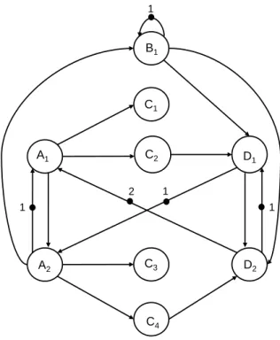
3.2 Equivalent HSDF graph for the SDF graph shown in figure 2.6b. The no-tation _𝑥𝑦 in the nodes denotes the_𝑦𝑡ℎ firing of a actor_{𝑥, where 𝑦 ∈ [1, 𝑞𝑥],}

𝑞𝑥 being the granularity of the actor 𝑥. . . . 27

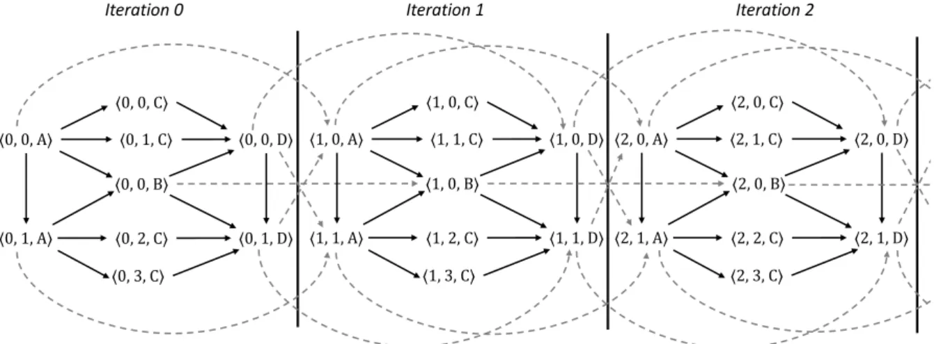
3.3 Symbolic execution trace of the SDF graph of Fig. 2.6b. Solid arcs are intra-iteration dependencies, dashed arcs are inter-iteration dependencies and the notation ⟨𝑛, 𝑘𝑖, 𝑖⟩ stands for the completion of the 𝑘_𝑖𝑡ℎ firing of an actor 𝑖 in the 𝑛𝑡ℎ iteration of the SDF graph, where 𝑛 ∈ ℕ, 𝑘𝑖 ∈ [0, 𝑞_𝑖), 𝑞_𝑖 being the granularity of the actor𝑖. . . . 28

3.4 Normalized representation of the SDF graph depicted in figure 2.6b . . . . 28

3.5 Counter example showing that theorem 3.2 is not a necessary condition for liveness. . . 29

3.6 A self-timed schedule of the timed SDF graph depicted in figure 3.1. . . . 30

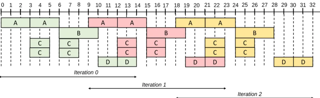
3.7 A SWP Schedule for the timed SDF graph depicted in figure 3.1. . . 32

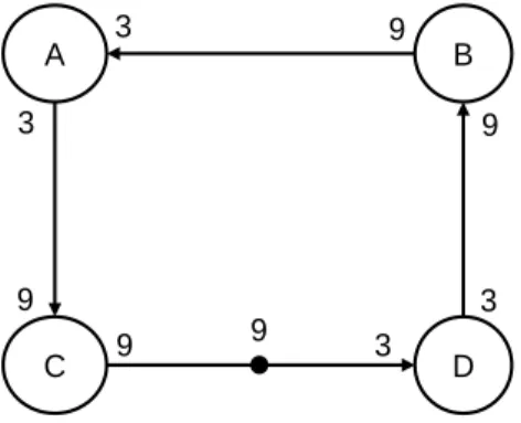
3.8 An example of architecture . . . 34

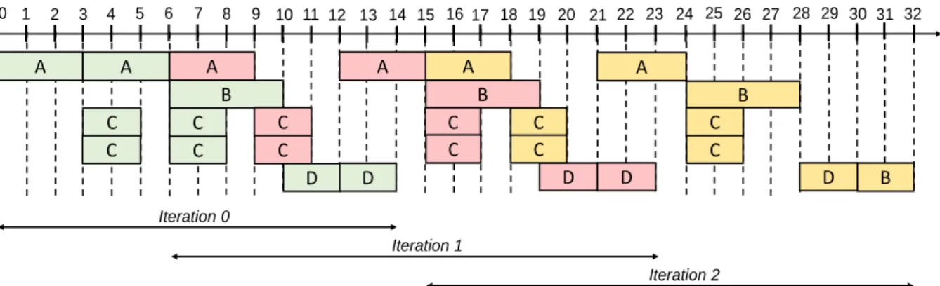
4.1 A SWP Schedule of period _{𝜆 = 10 and latency T}∗ =14 for the timed SDF graph depicted in figure 3.1. . . 50

LIST OF FIGURES

5.1 An optimal scheduling solution obtained for the non-timed SDF graph and

the architecture of our running example. . . 57

5.2 An illustration example for the Heuristic GS (algorithm 2). . . 61

5.3 Illustration of the Heuristic HCS. . . 68

6.1 Results of BG for synthetic Benchmarks . . . 73

6.2 Results of average Speedup for synthetic Benchmarks . . . 73

6.3 Results of BG for StreamIt Benchmarks . . . 76

List of Tables

2.1 Comparison of dataflow models. Notations: excellent (++++), very good (+++), good (++), less good (+) . . . 17

3.1 Related works on SWP scheduling of loops modeled by dataflow graphs . . 36

5.1 Scheduling list for the acyclic dependency graph of Fig. 5.3b . . . 69

6.1 Results of Average Solving Times (sec) for different synthetic benchmarks . 72

6.2 Benchmarks Characteristics . . . 74

List of Symbols

• _{ℤ: the set of integers.}

• ℕ the set of positive integers. • ℚ+: the set of positive rationals.

CHAPTER 1

Introduction

Contents

1.1 General Context and Problem Statement . . . . 2

1.2 Contributions . . . . 4

1.1. General Context and Problem Statement

1.1 General Context and Problem Statement

During the past decades, advances in hardware and software technologies have led to the development of modern computing systems called cyber-physical systems (CPSs). These systems are attracting a lot of attention in recent years and are being considered as innova-tive technologies that can improve human life and address many technical, socio-economical and environmental challenges.

What are CPSs? There is a plethora of definitions in the literature [2, 4, 6,7,8,9] that

may agree with our vision. We believe that CPSs are integrations of distributed comput-ing components which interact with each other through wired or wireless communication resources to sense and control physical processes. Unlike traditional embedded systems (smartphones, digital watches, etc.), which are designed as standalone devices, the focus in a CPS is on networking several devices or sub-systems and commanding them remotely in order to interact with physical processes. CPSs find applications in a wide range of domains including manufacturing, healthcare, environment, transportation. In the manufacturing industry, they are being introduced to characterize the upcoming of the fourth industrial revolution, frequently noted as Industry 4.0 [2,4,5, 6]. A manufacturing CPS (also called cyber-physical production system) is a production system where equipment such as robots, automated guided vehicles (AGVs), sensors and controllers interact with each other to control and monitor manufacturing operations at all levels of the production, from physi-cal transformation processes through machines up to logistics network. In the healthcare sector, CPSs are being used to remotely monitor the health conditions of in-hospital and in-home patients and to provide healthcare services [7]. A healthcare CPS is a system that collects the health data of patients through various medical sensors, transmits these data to a gateway via a wired or a wireless communication medium, stores the data in a cloud server and makes these data accessible to caregivers. In environment and transportation areas, large scale CPSs named smart cities [3] are being deployed to improve the service efficiency and quality of life in the cities. A smart city is one including digitally connected service systems such as transportation, power distribution and public safety systems, which are integrated using various information and communication technologies. In such a city, we will travel in driverless cars that communicate with each other on smart roads and in planes that coordinate to reduce delays. Homes and offices will be powered by a smart grid that use sensors to analyze the environment and optimize energy in real time.

Design Requirements. Each of the CPSs previously presented consists of multiple

es-1.1. General Context and Problem Statement

sentially loop-intensive applications —i.e. applications that perform repetitive computa-tions —that generate a huge volume of data processed by the computing platforms. These platforms are usually multiprocessor systems that include a finite number of heterogeneous processing resources, each communicating with the other ones through different communi-cation means. Thus, the computations of software applicommuni-cations can be easily parallelized by distributing data across different processing resources. An important design requirement of CPSs is that the processing resources of a computing platform may be shared between the computations of one or more applications. This requirement can lead to resource conflicts and/or communication bottlenecks when different computations need to access the same resources at the same time, and thus, it can cause a loss of parallelism and a noticeable deterioration of performance achievable by the software applications. To prevent such a situation, CPS designers often need to explore the parallelization choices of computations to different types of multiprocessor architectures. For this purpose, the design approaches for CPSs should be based as much as possible on formal models of computation that deal both with time, concurrency and parallelism. These models should be implementable and analyzable so that the designers may use them to predict the timing behaviour of CPS applications and to provide performance guarantees for these applications at design stage. Among the popular models of computation, dataflow models are of high interest.

Dataflow models. Dataflow modeling paradigm is characterized by a data-driven style of

control where data are processed while flowing through a networks of computation nodes. A dataflow model is a directed graph where nodes (called actors) describe the computations performed by a loop-intensive application and edges are FIFO channels that describe the dependency relations between the computations. When an actor fires, it consumes a finite number of data tokens and produces a finite number of data tokens. A set of firing rules indicates when the actor is enabled to fire. Dataflow models are often classified into dynamic and static models. Dynamic dataflow models are known to be more expressive than static dataflow models. However, the Turing-completeness and non-decidability of these models has motivated the research community to adopt static dataflow models when it comes to implement and analyze the behaviour of an application. Various types of static dataflow models exists. One of the most known is synchronous dataflow (SDF) model. In a SDF graph, the number of tokens consumed and produced by each actor at each firing is predefined at design stage. SDF graphs has been traditionally used to design streaming and multimedia applications. There interests are increasingly growing nowadays in the CPS design because of their semantics that enables to describe different levels of parallelism in loop-intensive applications and to analyze the timing behaviour and performance of these

1.2. Contributions

applications through the construction of static-order schedules (i.e. infinite repetitions of firing sequences of actors) with bounded FIFO channels.

Scheduling. Scheduling a static dataflow graph consists in finding “when” the firings of

each actor must be executed. An optimal schedule of a static graph is a schedule that achieves an optimal performance goal. Interesting performance indicators often analyzed to evaluate the optimality of schedules for static dataflow graphs are usually throughput and latency. From a CPS perspective, the study of these metrics is important to predict the timing behaviour of CPS applications and to provide performance guarantees for these applications. Scheduling strategies for static dataflow graphs can be classified into timed schedules (also called as soon as possible schedules) and periodic schedules. In a self-timed schedule, the instances of actors are executed as soon as possible the required data are available while in a periodic schedule, the instances of actors are executed according to a fix time period. Self-timed schedules are known as scheduling strategies that achieve optimal throughput for static dataflow graphs. However, these schedules are more difficult to implement than periodic schedules. A common way to get around the implementation complexity of self-timed schedules is to implement software pipelined (SWP) schedules [33,

60]. SWP schedules are a subclass of periodic schedules widely used to analyze the timing behaviour of loop-intensive applications. These schedules provide the same guarantees than self-timed schedules in terms of throughput achievement.

Problem statement. In this thesis, we address the following problem: given a CPS

application modeled by a SDF graph and a CPS platform described by a heterogeneous multiprocessor architecture with a fixed number of communicating processing resources, how can one construct an optimal SWP schedule that achieves the highest performance of the SDF graph under the resource and communication constraints of the given architecture? Scheduling an application graph under resource and/or communication constraints is a NP-hard problem [29,59]. Therefore, the problem tackled by this thesis is NP-hard. The main objective of the thesis is to propose efficient strategies to solve this scheduling problem.

1.2

Contributions

In order to solve the problem stated above, we have made several contributions to the scheduling of SDF graphs. Our main contributions are the following ones:

• First, we characterize the set of admissible SWP schedules that achieve optimal throughput/latency for timed SDF graphs and we propose linear programming

mod-1.3. Thesis Organization

els to compute these schedules.

• Secondly, we show that the problem can be model as an integer linear programming (ILP) model with precise optimization constraints and objective. The ILP model accommodates pipeline, task and data parallelism in SDF graphs and it characterizes the set of SWP scheduling solutions that achieves optimal throughput.

• Thirdly, we propose a guaranteed decomposed SWP scheduling heuristic, that genera-tes approximated SWP scheduling solutions for the problem.

1.3

Thesis Organization

This thesis is organized into two parts:

• Part 1. This part presents the motivations, state-of-the-art and a detailed formu-lation of the problem tackled by this thesis. The part consists of two chapters. The first chapter (chapter 2) gives a quick overview of design requirements and tools for cyber-physical systems. In this chapter, we show why heterogeneous multiproces-sor architectures and synchronous dataflow (SDF) model are suited to the design of cyber-physical systems and we present the motivations that pushed us to be inter-ested in the scheduling of SDF graphs on multiprocessor architectures under resources and communication constraints. In the second chapter (chapter 3), we review the basics of the SDF model, we formulate the main problem tackled by this thesis and we present some related works.

• Part 2. In this part we present our contributions. The part is organized into four chapters. In the first chapter (chapter 4), we propose a theorem that characterizes the set of admissible SWP schedules for timed SDF graphs. In this chapter, we also present two linear programming models, one enabling to compute SWP schedules that achieve maximum throughput for timed SDF graphs and the other to compute SWP schedules that achieve minimum latency. In the second chapter (chapter 5), we extend the characterizations made in chapter 4 to formulate an ILP model used to generate SWP scheduling solutions that achieve maximum throughput for SDF graphs on heterogeneous multiprocessor architectures under resource and communi-cation constraints. In this chapter, we also present our decomposed SWP scheduling heuristic that generates approximated scheduling solutions for the resource- con-strained and communication-concon-strained scheduling problem. In the third chapter

1.3. Thesis Organization

(chapter 6), we validate of our contributions thanks to experimental results made with synthetic benchmarks and real-world application benchmarks. In the fourth chapter (chapter7), we summarize our contributions and present some open research challenges.

Part I

Motivations, State-of-the-Art and

Problem Formulation

CHAPTER 2

Background and Motivations

Contents

2.1 Introduction . . . . 9

2.2 Architecture of Cyber-Physical Systems . . . . 9

2.3 Parallel Programming Paradigm . . . 12 2.3.1 Multithreading Programming Models. . . 12 2.3.2 Dataflow Programming Models . . . 15

2.4 Deployment of Loop-Intensive Applications . . . 17 2.4.1 Modeling and Exploitation of Parallelism . . . 18 2.4.2 Scheduling under resource and communication constraints . . . . 19

2.1. Introduction

2.1 Introduction

This chapter presents the background and motivations of this thesis. In the chapter, we give a quick overview of cyber-physical systems, the multiprocessor architectures, the parallel programming models and we present the motivations that pushed us to be interested in the scheduling of SDF graphs on heterogeneous multiprocessor architectures under resources and communication constraints.

2.2

Architecture of Cyber-Physical Systems

Cyber-physical systems (CPSs) can generally be represented as a control-loop structure like that depicted in figure 2.1. There are three parts in this structure. Firstly, there is a physical plant, which represents the “physical part” of a CPS. This part can include human operators, mechanical parts, biological or chemical processes. Secondly, there are computing platforms, each with its own sensors, computing features and/or actuators. Thirdly, there is a network fabric, which provides the mechanisms for the platforms to communicate. Together, the platforms and the network fabric constitute the “cyber part” of a CPS. Figure 2.1 illustrates a CPS structure composed with two computing platforms.

Figure 2.1: Example Structure of a CPS (Lee & Seshia [8])

Platform 2 measures the processes in the physical plant using sensor 2 and it controls the physical plant via actuator 1. The box labelled “Computation 2” represents a control application which uses the data collected by sensor 2 data to generate the command laws that trigger the behaviour of the actuator.“Computation 3” realizes an additional control

2.2. Architecture of Cyber-Physical Systems

PU1 PU2

PU3 PU4

(a) Homogeneous architecture

PU2 PU3

PU1

PU4

(b) Heterogeneous architecture

Figure 2.2: Illustration of different types of multiprocessor architectures

law, which is merged with that of “Computation 2” and Platform 1 makes additional measurements via sensor 1, and sends messages to Platform 2 via the network fabric.

A common requirement of a CPS is the need of processing a large volume of data collected by various sensors in order to control the physical plant at real-time. For this purpose, multiprocessor computing architectures are often implemented to parallelize the computations of CPS. Over the past decades, different types of multiprocessor architec-tures have been proposed to parallelize computations in many computer systems. These architectures can be classified into homogeneous and heterogeneous architectures. Figure

2.2 gives a graphical illustration of these different types of architectures. A homogeneous multiprocessor architecture includes multiple processing units (PUs) which have the same micro-architecture and/or provide the same computing performance while a heterogeneous architecture combines different types of PUs each having a specific micro-architecture and/or a providing specific computing performance. A systematic question that arises when designing the “cyber” part of a CPS, is whether a homogeneous or heterogeneous architectures should be used. In order to provide an answer to this question, Amdahl’s law [13] can be used to compute the performance provided by both types of systems. This law finds the maximum expected improvement of an overall computer system when only a part of the system is improved. Let speedup be the original execution time of a software program divided by an enhanced execution time. The modern version of Amdahl’s law states that if a fraction 𝑓 of a software program is enhanced by a speedup 𝑆, then the overall speedup of this program is given by:

𝑆𝑝𝑒𝑒𝑑𝑢𝑝𝑒𝑛ℎ𝑎𝑛𝑐𝑒𝑑(𝑓 , 𝑆) = 1

(1 − 𝑓 ) + _𝑆𝑓

(2.1)

In the context of multicore and multiprocessor systems, the authors in [14] have provided a corollary of Amdahl’s law. Let us consider a multiprocessor system (or a multicore

2.2. Architecture of Cyber-Physical Systems 0 2 4 6 8 10 12 14 16 1 2 4 8 1 6 f=0,5 f=0,9 f=0,975 f=0,99 f=0,999 Values of r Sp ee d u p

(a) Homogeneous with n=16

0 10 20 30 40 50 60 1 2 4 8 1 6 3 2 6 4 f=0,5 f=0,9 f=0,975 f=0,99 f=0,999 Values of r Sp ee d u p (b) Homogeneous with n=64 0 50 100 150 200 250 1 2 4 8 1 6 3 2 6 4 1 2 8 2 5 6 f=0,5 f=0,9 f=0,975 f=0,99 f=0,999 Values of r Sp ee d u p (c) Homogeneous with n=256 0 2 4 6 8 10 12 14 16 1 2 4 8 1 6 f=0,5 f=0,9 f=0,975 f=0,99 f=0,999 Values of r S p eedu p (d) Heterogeneous with n=16 0 10 20 30 40 50 60 1 2 4 8 1 6 3 2 6 4 f=0,5 f=0,9 f=0,975 f=0,99 f=0,999 Values of r S p eedu p

(e) Heterogeneous with n=64

0 50 100 150 200 250 1 2 4 8 1 6 3 2 6 4 1 2 8 2 5 6 f=0,5 f=0,9 f=0,975 f=0,99 f=0,999 Values of r Sp e e dup (f) Heterogeneous with n=256

Figure 2.3: Speedup of homogeneous and heterogeneous multiprocessor/multicore systems. machine) with_{𝑛 processors (or cores). Under Amdahl’s law, the overall speedup of such a} system depends on the fraction 𝑓 of software program that can be parallelized, the number 𝑛 of processors in the system and the number 𝑟 of base processors that can be combined to build one bigger processor (or core). In the case of a homogeneous multiprocessor system, one processor is used to execute sequentially the software program at performance𝑝𝑒𝑟 𝑓 (𝑟) and𝑛/𝑟 processors are used to execute in parallel the program at performance perf (r)×𝑛/𝑟. Thus, the overall speedup obtained with this system is given by:

𝑆𝑝𝑒𝑒𝑑𝑢𝑝ℎ𝑜𝑚𝑜𝑔𝑒𝑛𝑒𝑜𝑢𝑠(𝑓 , 𝑛, 𝑟) = _{1− 𝑓} 1

perf(r)+

𝑓 · 𝑟 perf(r)· 𝑛

(2.2)

In the case of a heterogeneous multiprocessor system, only the processor with more com-putation resources is used to execute sequentially at performance perf(r). In the parallel fraction, however, it gets performance perf(r) from the large processor and performance 1 from each of the𝑛 −𝑟 base processors. Thus, the overall speedup obtained with this system is given by: 𝑆𝑝𝑒𝑒𝑑𝑢𝑝ℎ𝑒𝑡𝑒𝑟𝑜𝑔𝑒𝑛𝑒𝑜𝑢𝑠(𝑓 , 𝑛, 𝑟) = _{1− 𝑓} 1 perf(r)+ 𝑓 perf(r)+ 𝑛 − 𝑟 (2.3)

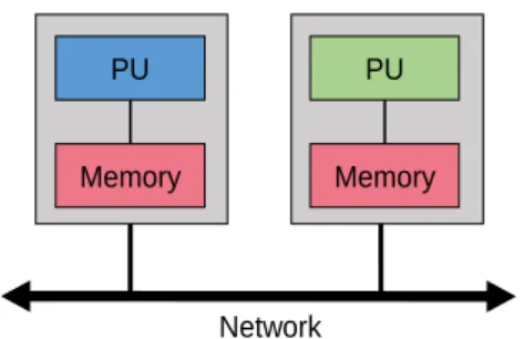
2.3. Parallel Programming Paradigm

PU

Memory PU

(a) Shared memory architecture

PU

Memory

PU

Memory

Network

(b) Distributed memory architecture

Figure 2.4: Multiprocessor architectures according to the memory access criteria Figure2.3 plots the speedup obtained for both homogeneous and heterogeneous multipro-cessors/multicore systems with respect to different values of the parameters _{𝑓 , 𝑛 and 𝑟. In} these plots, we assume that perf(f) = √_{𝑟 as done in [}14]. As it can be seen, for a same number of processing units, the speedups obtained with a heterogeneous system is much better than those obtained with a homogeneous system. This observation is an important reason for using heterogeneous multiprocessor architectures for CPSs design.

2.3

Parallel Programming Paradigm

Previously shown, heterogeneous multiprocessor architectures have an attractive advantage to carry out efficiently parallel computations in CPSs. In order to efficiently exploit the potential of these architectures, different hardware programming mechanisms have been proposed. However, their utilization is extremely complex for designers and programmers. To overcome this complexity, many programming approaches focus on the specification of software applications intended to run on these computer architectures. Thus, a plethora of application programming models have been proposed to allow users to write their software programs and to specify parallelism in these programs. These models can be classified into multithreading and dataflow models.

2.3.1

Multithreading Programming Models

Multithreading is a programming paradigm based on the utilization of threads to specify concurrency and parallelism in software programs. A thread is a way of making a program to execute two or more computational tasks at the same time. A thread consists of its own program counter, its own stack and a copy of registers of central processing unit (CPUs), but it shares other things like the code that is executing, heap and some data structures. Several multithreading programming models exist. PThread, OpenMP, MPI and OpenCL

2.3. Parallel Programming Paradigm

are four of the well-known multithreading programming models.

Pthread. Pthread also known as POSIX thread [20] is a low-level application

program-ming model for writing concurrent software programs for shared-memory computer archi-tectures (refer to figure 2.4a). It consists of a library of functions used to define threads accessing to a shared-memory space. The programming model is built on the top of imper-ative programming language like C and it supports different variants of operating systems including Unix, Windows and Mac OS. Although Pthread has its place in specialized sit-uations, the mechanisms for synchronizing threads is not explicitly defined, which makes the utilization of this programming model difficult for programmers to develop correct and maintainable computer programs [16,15].

OpenMP. OpenMP [17] is a high-level programming model to write parallel software

programs for shared-memory computer systems ranging from desktops to supercomputers. The implementation of OpenMP exists for three different programming languages including Fortran, C and C++. Contrary to POSIX Thread, the utilization of threads OpenMP is highly structured and threads are implicitly synchronized. In an OpenMP program, when an executing thread encounters a “parallel” directive, it will create a group of threads and become the master thread of this group. Then the group of threads executes the program code assigned to it. When the group has terminated its execution, the master thread collects the results from the group of threads and serially executes from that point on. For example if a “for” loop that will iterate over an array containing 100 elements would be parallelized on a processor with 4 cores, OpenMP will be used to create four threads and execute one thread on each core. The “for” loop will be wrapped in a parallel directive where the limit of threads is four. Then, when the initial thread encounters this directive a fork would occur, four tasks would be created and the goal for each task is to iterate over a subset of the array. This will increase the performance by four times, sometimes more if it benefits from super-linear speedup [17]. Recently, OpenMP has been extended for heterogeneous multiprocessor architectures, which makes it one of the two predominant models for programming many parallel computing systems, the other being Message Passing Interface (MPI) [18].

MPI. As opposed to Pthread and OpenMP, MPI [18] is a programming model that was

developed for writing portable software programs for distributed-memory computer archi-tectures (refer to figure 2.4b). Similar to OpenMP, the implementations of MPI is also available for C, C++, and Fortran programming languages. Programming with MPI have an attractive advantage that it provides point-to-point and collective communication

mod-2.3. Parallel Programming Paradigm

els to specify the communicating threads, without having to manage their synchronization. In an MPI program, a computation comprises one or more threads that communicate by calling library routines to send and receive messages to other threads. In most MPI imple-mentations, a fixed set of threads is created at the program initialization, and one thread is created per processor. However, these threads may execute different programs. Hence, the MPI programming model is sometimes referred to as a multiple program multiple data model to distinguish it from the single program multiple data model in which every process-ing element executes the same program. MPI programmprocess-ing model remains the dominant model used for designing parallel computing application today[19].

OpenCL. OpenCL [21] is a low-level standardized programming model designed to

sup-port the development of sup-portable software programs intended to run on heterogeneous computing systems with shared memory architectures. OpenCL views a computing sys-tem as a set of devices which might be central processing units (CPUs), graphics processing units (GPUs), digital signal processors (DSPs) or field-programmable gate arrays (FPGAs) attached to a host processor (a CPU). OpenCL programs are divided into host and kernel code. In the host program, kernels and memory movements are queued into command queues associated with a device. The kernel language provides features like vector types and additional memory qualifiers. A computation must be mapped to work-groups of work-items that can be executed in parallel on the processing cores of a device. OpenCL programming model is a good option for mapping threads on different processing units. However, it might be a too low-level programming model for many application-level pro-grammers who would be better served using MPI and OpenMP programming models.

In summary, all of the above mentioned programming models won for general purpose parallel computer systems which involve either shared memory or distributed memory communication mechanisms. However, their utilization is inappropriate in the context of CPSs because of the non-determinism of thread-based programs which can lead to communication overheads, high latencies and/or low throughput and thus decrease the performance of many CPS applications.

2.3. Parallel Programming Paradigm A 2 B (a) KPN 1 A 2 1 B (b) HSDF 3 A 2 2 B (c) SDF A [1] 2 [1,2] B (d) CSDF

Figure 2.5: Examples of the most popular dataflow model.

2.3.2 Dataflow Programming Models

Dataflow programming is a visual programming paradigm that appeared with Karp and Miller [66] in the middle of 1960s to specify parallelism in computer programs and to analyze the behaviour of these programs. A dataflow program is described as a directed graph where nodes (called actors) represent computations and arcs (called channels) represent the streams of data flowing between the computations. Actors can communicate with each other by exchanging data onto the channels. Such data are seen as discrete streams of tokens usually represented by dots. A channel may be initialized with a fix number of tokens to describe loop-carried dependency between the execution instances of computations. The quantity of tokens over a channel is called marking and an actor can fire whether there is a sufficient quantity of tokens on its input channels. Dataflow programming models provide high-level abstractions for specifying, analyzing and implementing the behaviour of a wide range of software applications. Nowadays, they are attracting a lot of interests in the design of CPS applications [8]. Various types of dataflow models exist. The most popular are Kahn process networks (KPN), homogeneous static dataflow (HSDF), synchronous dataflow (SDF) and cyclo-static Dataflow (CSDF). Figure 2.5 gives an illustration of each of these models.

KPN. KPN is dynamic dataflow model proposed in 1974 by Gilles Kahn [63]. A KPN

model (figure 2.5a) is composed of actors linked by unbounded FIFO channels, each con-necting a unique pair of actors. Each actor has a sequential behaviour and cannot produce tokens of data on more than one channel at a given time. The firing rules of actors is based on blocking reads and non-blocking writes semantics. This means that an actor can produce a token of data on a channel whenever it wants and must wait when it tries to consume a data token from an empty channel until this data arrives on this channel. The non-blocking write semantics ensures that actor can produce tokens continuously on the channels while the blocking read semantics ensures that any execution order of actors

2.3. Parallel Programming Paradigm

will yield the same histories of tokens on the channels. KPN is a Turing-complete model [56] that has a high expressiveness to provide a fine-grained description of many computer programs which are inherently partitioned into separate tasks communicating via streams of data. However, like many Turing complete models, KPN is not decidable, i.e. it does not allow deadlocks and performance analysis of computer programs at design time.

HSDF. This model is introduced in 1968 by Reiter [65]. HSDF (figure 2.5a) is a static

dataflow model also known as single-rate dataflow model in the signal processing commu-nity or marked graph in the Petri Net commucommu-nity. This model imposes limitations on the KPN model in order to make deadlocks and performance analysis possible for the com-puter systems at design time. An HSDF model consists of actors connected with bounded First In First Out (FIFO) channels. The execution instances of actors specifies how many tokens are produced and consumed on each channel. The number of tokens consumed and produced by actors is predetermined and specified on the input and output ports of the channels. When an actor fires, it a consumes a constant number of data tokens from input channels and produces the same number of tokens on output channels. HSDF is less expressive than KPN, however, the bounded capacity of FIFO channels and the constant number of consumption and production rates makes this model more analyzable and easier to implement than the KPN model.

SDF. This model is presented in 1987 by Lee and Messerschmitt [61]. SDF (figure2.5c) is

a static dataflow model also known as multi-rate dataflow model in the signal processing community or weighted event graph in the Petri Net community. Similar to the HSDF model, it consists of actors connected by bounded FIFO channels. However, it extends the HSDF model by allowing the specification of different production and consumption rates on the channels. Thus, actors can produce and consume tokens at different rates. In a SDF model, when an actor fires, it consumes a fixed number of tokens —which is predetermined in design time —from each of its incoming channels, and it produces a fixed number of tokens on each of its outgoing channels. Figure 2.5c shows an example of SDF graph composed of two actors (𝐴 and 𝐵) linked by a single channel. The production and consumption rates are indicated respectively at the source and the end of the channel. It should be noted SDF models are more expressive and compact than HSDF models.

CSDF. This model is a static dataflow graph introduced in 1995 by Bilsen [46]. It can be

seen as an extension of the SDF model. In a CSDF model (figure2.5d), the production and consumption rates associated to the FIFO channels are decomposed into finite sequences (also called phases) which may change periodically between the execution instances of

2.4. Deployment of Loop-Intensive Applications

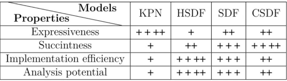
Table 2.1: Comparison of dataflow models. Notations: excellent (++++), very good (+++), good (++), less good (+)

Properties Models KPN HSDF SDF CSDF

Expressiveness _{+ + ++ + ++ ++}

Succintness + ++ + + + + + ++

Implementation efficiency + + + ++ + + + ++

Analysis potential _{+ + + ++ + + + ++}

actors. Each actor has a finite number of phases and each phase characterize the number of tokens produced or consumed by this actor. For instance, figure2.5dillustrates a CSDF with two actors (𝐴 and 𝐵) connected by a single channel. Actor A has an unique production phase where it produces a single token onto the channel while Actor_{𝐵 has two consumption} phases where it consumes one token in the first phase and two tokens in the second phase. CSDF is not more expressive than SDF but it is more succinct for describing the computer programs of very large parallel computer systems. However, the complexity to analyze CSDF programs is larger than the analysis complexity of a SDF programs with an equal number of actors [38].

To summarize, SDF, HSDF, and CSDF are static dataflow models that impose a re-striction on the KPN model to allow static analysis of computer systems at design time. A detailed comparison of all of these dataflow models have been provided by Stuijk in 2007 [38] according to four criteria including expressiveness, succinctness, implementation efficiency and analysis potential. Table 2.1 presents a summarized comparison of these dataflow models. From this table, we can clearly see that, SDF model is the one that provides a good compromise. In this thesis, we will focus on the utilization of SDF graphs to specify parallelism in CPS applications and to analyze the performance achievable by these applications on heterogeneous multiprocessor architectures.

2.4

Deployment of Loop-Intensive Applications

A key aspect in the design of a CPS is the software deployment through which the com-putations of CPS applications are scheduled and mapped on the PUs of heterogeneous multiprocessor architectures. Scheduling a computation consists to find “when” this com-putation must start its execution while mapping a comcom-putation consists in finding “where” the computation should be executed. The scheduling and mapping of computations for

2.4. Deployment of Loop-Intensive Applications

A[k] ← A[k-1]⊙ D[k-3]

B[k] ← B[k-1]⊙ A[2k] ⊙ A[2k+1] C[k] ← A[floor(k/2)]

D[k] ← D[k-1]⊙ B[floor(k/2)] ⊙ C[2k] ⊙ C [2k+1] (a) Loop-intensive program

2 1 2 2 1 1 2 1 1 1 A B C D 3 1 1 1 1 1 1 1 1 1 (b) SDF graph

Figure 2.6: A loop-intensive program and its SDF representation

CPS applications depend on many parameters which include for instance, the number of PUs available on the multiprocessor architectures, the worst-case execution times of com-putations onto the PUs and the inter-PUs communication latencies. In addition to these parameters, loop-carried dependencies should be considered. Actually, loops usually be-ing the most time-critical parts of many software applications, the performance achievable by the applications depends on the optimal execution of loops embedded in the software programs. Therefore, to predict the timing behaviour of CPS applications and to provide performance guarantee at design stage, there is a need of exploring and exploiting the parallelism embedded in the execution pattern of loops. For this purpose, we will show that SDF graphs can be very helpful.

2.4.1

Modeling and Exploitation of Parallelism

SDF graphs provide various mechanisms to model and exploit different levels of parallelism such as data, task and pipeline parallelisms in loop-intensive programs. Actually, the actors of a SDF graph that describes a loop-intensive program can be specified either as stateful or as stateless. A stateful actor is an actor whose execution instances are scheduled in a sequential order while a stateless actor is an actor whose execution instances are scheduled out of order, or in parallel across different PUs. These types of actors respectively enable to specify pipeline and data parallelisms in loop-intensive programs. A stateful actor is often described as a node with a self-loop channel, where the channel consists of a fixed number of tokens that represents the distance separating the successive execution instances of the stateful actor. Figure 2.6 depicts a loop-intensive program and its equivalent SDF graph.

2.4. Deployment of Loop-Intensive Applications

The loop-intensive program of four instructions and four computing functions (𝐴, 𝐵, 𝐶 and 𝐷). Each instruction is a logical and/or arithmetic operation that describes one or several dependency relations between the different invocations of the functions. For instance, the instruction_{𝐴[𝑘] ← 𝐴[𝑘 −1] ⊙ 𝐷 [𝑘 −3] is an arithmetic (or logical) operation that describes} two dependency relations: a dependency from the _{(𝑘 − 1)}𝑡ℎ invocation of actor A to the_𝑘𝑡ℎ invocation of this actor and a dependency from the _{(𝑘 − 3)}𝑡ℎ invocation of actor _{𝐷 to the} 𝑘𝑡ℎ _{invocation of actor A. This loop-intensive program is graphically described by the SDF}

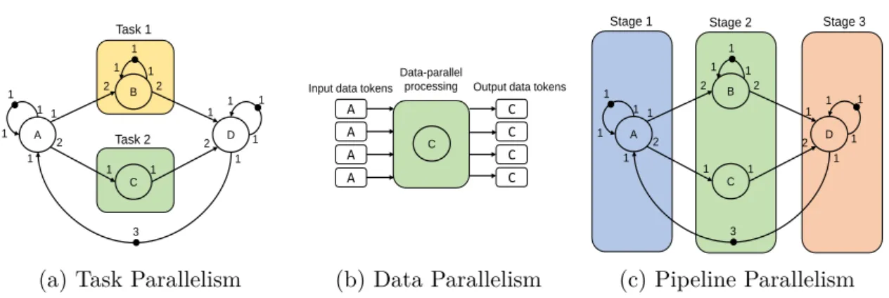
graph shown in Fig. 2.6b. This graph consists of four actors (𝐴, 𝐵,𝐶, 𝐷), each describing a computing funtion of the program. Actors𝐴, 𝐵 and 𝐷 are stateful actors while actor 𝐶 is a stateless actor. All of these actors are connected by a set of channels, each describing the flows of data exchanged between the computations, and some containing an initial number of tokens describing the distance separating the successive execution instances of connected actors. When deploying this graph on a multiprocessor architecture, data parallelism can be exploited by scheduling and mapping the execution instances of the actor_{𝐶 on a} data-parallel processor or on different PUs. At the same time, pipeline data-parallelism can be exploited by scheduling and mapping the execution instances of a stateful actor on different PUs in such a way that the successive executions of these execution instances can overlap over time. Alongside with data and pipeline parallelisms, task parallelism can also be exploited by scheduling and mapping the execution instances of actors𝐵 and 𝐶 on different PUs. Figure 2.7 illustrates the exploitation of these three types of parallelisms. The joint exploitation of task, data and pipeline parallelisms is known to improve the performance achievable by loop-intensive applications [40]. Therefore, to ensure performance guarantee for CPS applications, it is important that the scheduling and mapping strategies for these applications exploit efficiently these three kinds of parallelisms.

The two most prominent performance measurements for applications modeled by SDF graphs are latency, which reflects the delay induced by a channel to transfer a token of data between dependent execution instances, and throughput, which indicates for each actor, the execution rate per unit time. From a CPS perspective, the study of these properties are of a high interest to characterize the timing behaviour of loop-intensive programs and to provide performance guarantee for CPS applications. Consequently, in this thesis, we focus on the characterization and analysis of these two performance metrics.

2.4.2 Scheduling under resource and communication constraints

An important design requirement for CPS applications is that, the heterogeneous multipro-cessor architectures on which the computations are intended to be deployed, must contain

2.4. Deployment of Loop-Intensive Applications 2 1 2 2 1 1 2 1 1 1 A B C D 3 1 1 1 _{1 1} 1 1 1 1 Task 1 Task 2

(a) Task Parallelism

C

A

Data-parallel processing Input data tokens

A A A C C C C

Output data tokens

(b) Data Parallelism 2 1 2 2 1 1 2 1 1 1 A B C D 3 1 1 1 1 1 1 1 1 1

Stage 1 Stage 2 Stage 3

(c) Pipeline Parallelism

Figure 2.7: Types of parallelism exploitable in the SDF graph shown in figure2.6b.

a finite number of processing and communication resources, and these resources have to be shared between the computations of one or more applications. This requirement can often lead to resource conflicts and/or communication bottlenecks when different computations need to access the same resources at the same time, and thus can cause a loss of parallelism and an deterioration of performance achievable by CPS applications. In order to prevent such a situation, there is a need of developing static scheduling and mapping strategies that can accommodate the resource and communication constraints of multiprocessor ar-chitectures to reduce in the early design stage of the applications, the over-allocation of resources needed for computations to meet their timing constraints. Since most of CPS applications are essentially loop-intensive applications, it is important that the schedul-ing strategies respect the loop-carried dependencies constraints of these application, and ensure that the performance achievable by a computation is not influenced by the other computations assigned to the same resources.

Scheduling computations with dependency relations on multiprocessor architectures un-der resource and/or communication constraints is a NP-complete problem well-known in the literature [29, 59]. Many authors have proposed several static scheduling approaches to tackle this problem with the goal of optimizing different performance metrics. A de-tailed survey of these approaches can be found in [29]. Among the existing works, there are a number [26, 24, 30, 38, 33, 48] that uses SDF graphs to tackle the problem. How-ever, most of these works are limited to the scheduling of SDF graphs on homogeneous multiprocessor architectures. Among the works [25, 32, 58] tackling the scheduling and mapping of static dataflow graphs on heterogeneous multiprocessor architectures, an im-portant number is limited to the scheduling of acyclic SDF graphs. Although these types of graphs can model many types of applications, they fail to model applications with cyclic dependencies. Since most of loop-intensive programs for CPS may contain cyclic

depen-2.5. Conclusion

dencies, the SDF graphs that describe these programs may consist of cycles like the SDF graph depicted in figure 2.6b. Consequently, a scheduling strategy for these graphs must deal with cyclic dependency constraints while satisfying both resource and communication constraints. Scheduling a cyclic SDF graphs on heterogeneous multiprocessor architectures under resource and communication constraints is a difficult problem rarely addressed in the literature. The main goal of this thesis is to propose efficient static scheduling strategies to tackle this difficult problem while ensuring performance guarantees in terms of throughput and latency.

2.5

Conclusion

In this chapter, we have presented the background and motivations that pushed us to be interested in the scheduling of SDF graphs on heterogeneous multiprocessor architectures under resource and communication constraints. In the next chapter we will review the basics of the SDF model and will present a succinct formulation of the main problem tackled by this thesis.

CHAPTER 3

State-of-the-Art and Problem Formulation

Contents

3.1 Introduction . . . 23

3.2 Synchronous Dataflow Graphs . . . 23 3.2.1 Definition . . . 23 3.2.2 Consistency Analysis . . . 24 3.2.3 Liveness Analysis . . . 25

3.3 Static Scheduling of Synchronous Dataflow Graphs. . . 29 3.3.1 Basic Definitions and Theorems . . . 29 3.3.2 Self-timed Schedules Versus Periodic Schedules . . . 30 3.3.3 Throughput Evaluation . . . 32 3.3.4 Latency Evaluation. . . 33

3.4 Problem Formulation and Related Works . . . 34 3.4.1 ILP-based Scheduling Approaches . . . 36 3.4.2 Scheduling Heuristics . . . 37 3.4.3 This Work. . . 38

3.1. Introduction

3.1 Introduction

In this chapter we review the basics of the synchronous dataflow (SDF) model, which was introduced informally in the previous chapter, then we formulate the problem tackled by this thesis and we succinctly describe our main contributions. The chapter is organized as follows. Section 3.2 presents basic definitions and structural properties of SDF graphs. Section3.3 reviews the static scheduling strategies for SDF models. Section 3.4presents a succinct description of the main problem tackled by this thesis as well as the related works.

3.2

Synchronous Dataflow Graphs

3.2.1 Definition

A SDF graph is a multi-rate dependency graph𝐺_𝑠𝑑𝑓 = (𝑉, 𝐸, 𝑃,𝐶, 𝑀0) where:

• 𝑉 is a finite set of nodes called actors.

• _{𝐸 ⊆ 𝑉}2 _{is a finite set of arcs representing First-in First-out (FIFO) channels.}

• _{𝑃 = {𝑝𝑒 ∈ ℕ}∗_{| 𝑒 = (𝑖, 𝑗) ∈ 𝐸} is the set of production rates given by the function} 𝑝 : 𝐸 → ℕ∗ _{that associates a production rate𝑝𝑒 with each channel𝑒 = (𝑖, 𝑗) ∈ 𝐸.}

• 𝐶 = {𝑐_𝑒 ∈ ℕ∗| 𝑒 = (𝑖, 𝑗) ∈ 𝐸} is the set of consumption rates given by the function 𝑐 : 𝐸 → ℕ∗ _{that associates a consumption rate 𝑐𝑒 with each channel𝑒 = (𝑖, 𝑗) ∈ 𝐸.}

• 𝑀0 = {𝑚0(𝑒) ∈ ℕ| 𝑒 = (𝑖, 𝑗) ∈ 𝐸} is the set of initial markings given by the function

𝑚0 :𝐸 → ℕ that associates a fixed number 𝑚0(𝑒) of tokens with each channel 𝑒 ∈ 𝐸.

2 1 2 2 1 1 2 1 1 1 3 1 1 1 1 1 1 1 1 1 A, 3 B, 4 C, 2 D, 2

3.2. Synchronous Dataflow Graphs

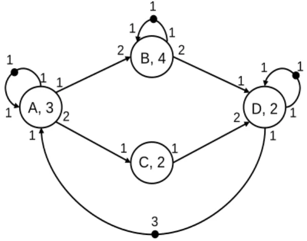
Timed Synchronous Dataflow Graph. A SDF graph𝐺_𝑠𝑑𝑓 is said timed if there exists

a function _{𝛿 : 𝑉 → ℕ}∗ that associates a duration _𝛿𝑖 with every actor _{𝑖 ∈ 𝑉 , where 𝛿𝑖} is the worst-case time to process a single execution instance of actor _{𝑖. Figure} 3.1 shows a graphical representation of a timed SDF graph, where each node models an actor and the worst-case processing time associated with the execution of each instance of this actor. For the rest of the manuscript, let us denote the execution instances of actors in terms of firings and let us denote the timed SDF graphs as𝐺_𝑠𝑑𝑓𝑡 = (𝑉, 𝐸, 𝑃,𝐶, 𝑀0, 𝛿).

3.2.2 Consistency Analysis

Consistency is a property that has been introduced initially by Lee and Messerschmitt [61] to ensure that actors of a SDF graph can be statically scheduled with a bounded number of tokens. Let us consider a SDF graph _{𝐺𝑠𝑑𝑓} = (𝑉, 𝐸, 𝑃,𝐶, 𝑀0) and let Θ be the topology

matrix of this graph, where _{Θ is a matrix of size |𝐸| × |𝑉 | defined by:}

Θ𝑒𝑖 =   𝑝𝑒 if𝑒 = (𝑖, 𝑗), 𝑗 ∈ 𝑉 −𝑐𝑒 if𝑒 = (𝑗, 𝑖), 𝑗 ∈ 𝑉 0 𝑜𝑡ℎ𝑒𝑟𝑤𝑖𝑠𝑒

𝐺𝑠𝑑𝑓 is said consistent if the rank of the matrix Θ is equal to |𝑉 | − 1. To illustrate this

property, let us consider the SDF graph shown in figure 2.6b. The topology matrix of this graph is given by:

Θ =       1 −2 0 0 2 0 −1 0 0 2 0 −1 0 0 1 −2 −1 0 0 1       A B C D e=(A, B) e=(A, C) e=(B, D) e=(C, D) e=(D, A)

Considering this topology matrix, it is possible to check that𝑟𝑎𝑛𝑘(Θ) = |𝑉 | −1 = 3. This means that the SDF model described by this matrix is consistent. Actually, the consistency property ensures the existence of a minimum vector _{𝑞 ∈ ℕ}∗|𝑉 | with coprime components such that _Θ.𝑞𝑇 = 0. This vector is called the repetition vector and its components are called granularities or repetition factors. The granularity_𝑞𝑖 of an actor_{𝑖 ∈ 𝑉 corresponds} to the minimum number of firings required for this actor to achieve a single iteration1_.

Thus, checking the consistency of a SDF model is equivalent to checking the existence of 1_{An iteration of a SDF graph is an execution sequence that brings back the graph to its initial state.}

3.2. Synchronous Dataflow Graphs

a repetition vector. For any SDF graph, the existence condition of a repetition vector is defined by:

𝑝𝑒 × 𝑞𝑖 =𝑐_𝑒 × 𝑞_𝑗 ∀𝑒 = (𝑖, 𝑗) ∈ 𝐸. (3.1)

Let us going back to the SDF graph depicted in figure2.6b, if we want to check the existence of a repetition vector for this graph, we must try to solve the following system of equations:

          1× 𝑞_𝐴 =1× 𝑞_𝐴 1× 𝑞𝐴 =2× 𝑞𝐵 2× 𝑞𝐴 =1× 𝑞𝐶 1× 𝑞𝐵 =1× 𝑞𝐵 2× 𝑞_𝐵 =1× 𝑞_𝐷 1× 𝑞_𝐶 =2× 𝑞_𝐷 1× 𝑞_𝐷 =1× 𝑞_𝐴 1× 𝑞_𝐷 =1× 𝑞_𝐷

The solution of this system of equations gives a repetition vector 𝑞 = [𝑞_𝐴, 𝑞_𝐵, 𝑞_𝐶, 𝑞_𝐷] = [2, 1, 4, 2] which proves that the SDF graph is consistent.

3.2.3

Liveness Analysis

Liveness is a property which ensures that every actor of a static dataflow model can be fired infinitely often without encountering deadlocks during the execution of the model. Liveness checking is a well-known problem extensively studied in the dataflow community. In 1971, Commoner et al. [64] have proposed the following theorem that serves as nec-essary and sufficient condition to ensure the liveness of marked graphs, which are named homogeneous synchronous dataflow (HSDF) graphs in the dataflow community.

Theorem 3.1 (Commoner et al. [64]). A HSDF graph is live if and only if the token count

of every directed circuit is positive.

Based on this theorem, Commoner et al. have proposed a polynomial-time algorithm —using depth-first search —to check the liveness of HSDF graph. The algorithm proceeds in two steps. In the first step, it removes every channel with non-zero marking from the HSDF graph and in the second step, it checks if resulting HSDF graph contains cycles. If the resulting graph is acyclic then the initial HSDF graph is live otherwise, it is not live.

3.2. Synchronous Dataflow Graphs

Algorithm 1: Transform a consistent SDF graph into a HSDF graph

Input: a consistent SDF graph_{𝐺𝑠𝑑 𝑓} = (𝑉, 𝐸, 𝑃,𝐶, 𝑀₀) with a repetition vector 𝑞. Output: an equivalent HSDF graph for_{𝐺𝑠𝑑 𝑓}

1 Let𝐺_{ℎ𝑠𝑑 𝑓} =(𝑉′, 𝐸′, 𝑀₀′) be an empty HSDF graph ; 2 foreach actor𝑖 ∈ 𝑉 do 3 for𝑘 = 1 . . . 𝑞_𝑖 do 4 Add node𝑎_𝑘 to𝑉′; 5 end 6 end 7 foreach channel𝑒 = (𝑖, 𝑗) ∈ 𝐸 do 8 for𝑘′=1. . . 𝑞𝑗 do 9 𝜋_{𝑖 𝑗}(𝑘′) ←⌈𝑘 ′_{· 𝑐𝑒 − 𝑚} 0(𝑒) 𝑝𝑒 ⌉ ; 10 𝑘 ← (𝜋_{𝑖 𝑗}(𝑘′) − 1) mod 𝑞_𝑖+ 1;

11 Add arc𝑒′=(𝑖_𝑘, 𝑗_𝑘′) to 𝐸′ and set_𝑚0(𝑒′) to −

⌊𝜋_{𝑖 𝑗}(𝑘′_{) − 1} 𝑞𝑖 ⌋ ; 12 end 13 end 14 return𝐺_{ℎ𝑠𝑑𝑓};

Contrary to HSDF graphs, liveness checking for SDF graphs is a problem whose time complexity is not polynomial. Two techniques exist to check liveness for a consistent SDF graph. The first technique consists in transforming the SDF graph into an equivalent HSDF graph and applying the algorithm of Commoner et al. [64] to check liveness for the HSDF graph. Many polynomial-time algorithms exist in literature to transform a SDF graph into an equivalent HSDF graph [28, 34, 58]. Figure 3.2 shows an equivalent HSDF graph for the SDF graph depicted in figure 2.6b. This HSDF representation also called linear constraint graph, is obtained with the algorithm of de Groote et al. [28], which enables to generate for any consistent SDF graph, an equivalent HSDF graph with fewer channels. The different steps of this algorithm are explicitly detailed by Algorithm 1. Considering the equivalent HSDF graph, the algorithm of Commoner et al. [64] can easily be applied to check liveness. For this liveness checking technique, it is important to mention that the transformation of a SDF graph to an equivalent HSDF graph may lead sometimes to a graph of exponential size, and thus can make exponential the time and space complexity of this technique. The second technique for liveness checking [39] consists in performing the symbolic execution of the SDF graph —i.e. to execute all the actors of the model exactly as many times as indicated by the repetition vector —until the graph reaches a repetitive