Exploration and Mapping using a Sparse Robot Swarm: Simulation Results

HAL Id: hal-02864274

https://hal.inria.fr/hal-02864274

Submitted on 11 Jun 2020

HAL is a multi-disciplinary open access

archive for the deposit and dissemination of

sci-entific research documents, whether they are

pub-lished or not. The documents may come from

teaching and research institutions in France or

abroad, or from public or private research centers.

L’archive ouverte pluridisciplinaire HAL, est

destinée au dépôt et à la diffusion de documents

scientifiques de niveau recherche, publiés ou non,

émanant des établissements d’enseignement et de

recherche français ou étrangers, des laboratoires

publics ou privés.

Exploration and Mapping using a Sparse Robot Swarm:

Simulation Results

Razanne Abu-Aisheh, Francesco Bronzino, Myriana Rifai, Brian Kilberg, Kris

Pister, Thomas Watteyne

To cite this version:

Razanne Abu-Aisheh, Francesco Bronzino, Myriana Rifai, Brian Kilberg, Kris Pister, et al..

Explo-ration and Mapping using a Sparse Robot Swarm: Simulation Results. [Research Report] RR-9349,

Inria. 2020, pp.17. �hal-02864274�

0249-6399 ISRN INRIA/RR--9349--FR+ENG

RESEARCH

REPORT

N° 9349

Mapping using a Sparse

Robot Swarm:

Simulation Results

Razanne Abu-Aisheh

, Francesco Bronzino, Myriana Rifai

,

Brian Kilberg, Kris Pister

, Thomas Watteyne

RESEARCH CENTRE PARIS

Razanne Abu-Aisheh

, Francesco Bronzino

, Myriana Rifai

,

Brian Kilberg

, Kris Pister

, Thomas Watteyne

Project-Team EVA

Research Report n° 9349 — June 2020 — 17 pages

Abstract: This research report is a companion to the following paper: Atlas: Exploration and Mapping with a Sparse Swarm of Networked IoT Robots. Razanne Abu-Aisheh, Francesco Bronzino, Myriana Rifai, Brian Kilberg, Kris Pister, Thomas Watteyne. Workshop on Wireless Sensors and Drones in Internet of Things (Wi-DroIT), part of DCOSS, 2020. It expands that paper by providing more detailed explanations and more complete results.

Exploration and mapping is a fundamental capability of a swarm of robots: robots enter an unknown area, explore it, and collectively build a map of it. This capability is important regardless of whether the robots are crawling, flying, or swimming. Existing exploration and mapping algorithms tend to either be inefficient, or rely on having a dense swarm of robots. This paper introduces Atlas, an exploration and mapping algorithm for sparse swarms of robots, which completes a full exploration even in the extreme case of a single robot. We develop an open-source simulator and show that Atlas outperforms the state-of-the-art in terms of exploration speed and completeness of the resulting map.

Key-words: Swarm, Exploration, Mapping, IoT, Micro-Robots.

∗_{Nokia Bell Labs, Paris, France.}

†_{BSAC, University of California, Berkeley, CA, USA} ‡_{Inria, Paris, France.}

Exploration and Mapping using a Sparse

Robot Swarm: Simulation Results

Résumé : This research report is a companion to the following paper: Atlas: Exploration and Mapping with a Sparse Swarm of Networked IoT Robots. Razanne Abu-Aisheh, Francesco Bronzino, Myriana Rifai, Brian Kilberg, Kris Pister, Thomas Watteyne. Workshop on Wireless Sensors and Drones in Internet of Things (Wi-DroIT), part of DCOSS, 2020. It expands that paper by providing more detailed explanations and more complete results.

Exploration and mapping is a fundamental capability of a swarm of robots: robots enter an unknown area, explore it, and collectively build a map of it. This capability is important regard-less of whether the robots are crawling, flying, or swimming. Existing exploration and mapping algorithms tend to either be inefficient, or rely on having a dense swarm of robots. This paper introduces Atlas, an exploration and mapping algorithm for sparse swarms of robots, which com-pletes a full exploration even in the extreme case of a single robot. We develop an open-source simulator and show that Atlas outperforms the state-of-the-art in terms of exploration speed and completeness of the resulting map.

Contents

3.3 Running the Simulation . . . 10

3.4 Simulation Outputs . . . 10

3.5 User Interface . . . 10

4 Limits of Ramaithitima in Sparse Swarms 11 5 Atlas 13 6 Simulation Results 13 6.1 Heatmaps . . . 13

6.2 Mapping Profiles . . . 13

6.3 Mapping Speed . . . 15

4 Abu-Aisheh et al.

1

Introduction

In “swarm robotics”, a potentially large number of robots carry out a task together, either because it cannot be carried out by a single robot, or it can be done more efficiently by a swarm. Applications for robotic swarms include carrying equipment throughout a warehouse, collaboratively repairing inaccessible structures, and localizing underground gas pipes.

Robots used for swarm robotics come in different shapes and sizes, including the dm-scale r-one from Prof. McLurkin at Rice University [1], the cm-scale kilobot from Prof. Nagpal at Harvard [2], and the mm-scale ionocraft from Prof. Pister at UC Berkeley [3]. These are shown in Fig. 1.

In this article, we are interested in a specific application: exploration and mapping. A swarm of robots is inserted into an unknown area, the robots explore the area, and while doing so, collectively create a map of it. Applications include finding survivors in a collapsed building after an earthquake, mapping out a building before entering in military applications, or exploring underwater caves.

We see exploration and mapping as a fundamental capability of a swarm of robots. Regardless of the final application of the swarm, or even whether it is composed of crawling, flying, or swimming robots, the swarm will most likely need to conduct some form of exploration and mapping. Creating a good map depends on many things: the ability for the robots to move well, their ability to sense the obstacles, the reliability of their communication, and the performance of the navigation algorithm that drives the exploration and mapping expedition.

This paper focuses on the latter. Our goal is to do a “hands-on survey” of the literature of exploration and mapping. We therefore develop a simulation platform, implement what we be-lieve are the most relevant proposals, and compare their performance. We discover that existing efficient proposals only generate complete maps when the swarm is very dense (e.g. hundreds of robots deployed on a medium-sized office floor). We therefore design Atlas, a systematic explo-ration and mapping algorithm specifically designed for sparse swarms, which creates complete maps even in the extreme case of a single robot.

The contributions of this paper are threefold:

• We develop a simulator specifically for comparing exploration and mapping algorithms. This simulator is published under an open-source license.

• We design Atlas, an exploration and mapping algorithm for sparse swarms.

• We extract the performance of Atlas, as well as three state-of-the-art algorithms, and present performance results on three representative scenarios.

The remainder of this paper is organized as follows. Section 2 surveys the most relevant related work. Section 3 details the open-source simulation platform developed for this paper. Section 4 shows by simulation that efficient algorithms only work for dense networks. Section 5 introduces Atlas, an algorithm specific to sparse swarms. Section 6 describes the simulation results. Finally, Section 7 summarizes the paper and discusses avenues for future work.

2

Related Work

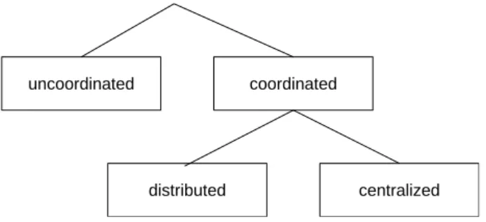
There are several ways to categorize exploration and mapping algorithms. Fig. 2 illustrates the taxonomy used in this paper, detailed below.

At the most fundamental level, one distinguishing feature is whether the robots are coor-dinated as the swarm of robots explores the area. In uncoorcoor-dinated algorithms, each robot in

Figure 1: Robots used in swarm robotics come in different shapes and sizes: the dm-scale r-one [1] (left), the cm-scale kilobot [2] (center), the mm-scale ionocraft [3] (right).

the swarm explores the area without coordinating with other robots. This makes for a very algorithmically simple solution, but yields inefficiencies, as multiple robots might for example be exploring the same area. In coordinated algorithms, the exploration of each robot is done to explicitly complement that of the others.

The latter category involves robots sharing information as they explore, which necessarily means some sort of (wireless) communication. Here again, there are different ways for the robots to share information. In distributed algorithms, robots only exchange information with other robots that are close by. The behavior of the swarm as a whole is “emergent”: many local (often simple) interactions between neighbor robots yield the overall behavior. Bio-inspired algorithms are often distributed, mimicking for example the behavior of ants in a colony. In centralized algorithms, the overall behavior of the swarm is explicitly driven by a central controller. This controller (e.g. a computer on the side of the area) receives information from the robots (the position of each robots, the partial map each has been able to explore, . . . ), and remotely controls the movement of each robot. As with any taxonomy, hybrid uncoordinated/coordinated or distributed/centralized approaches are of course possible.

Huang et al. [4] propose an uncoordinated algorithm for a swarm of robots to localize chemical leakages or radiation in a factory. The authors define three main stages. In the “random walk” stage, robots move forward at a constant speed in random directions and continuously investigate the environment using their sensors. In the “obstacle detected” stage, robots change the speed of their left and right motors depending on which sensor is stimulated. This causes the robot to change direction, before resuming random walk. Finally, in the “target detected” stage, the robot stops for a short period of time to carefully investigate the content of the detected target, record the relative position of this target, and continue with random walk. The resulting behavior is that robots progress in random directions, detect obstacles, then continue in a different random direction.

“Random walk” is a canonical form of uncoordinated exploration algorithms. Kegeleirs et al. [5] compare five flavors of random walk: Brownian motion, correlated random walk, Lévy walk, Lévy taxis, and ballistic motion. The authors implement all five on a swarm of 10 wheeled mobile robots, let them map out two types of lab environments, and quantify the quality of the maps the swarm generates. They conclude that ballistic motion yields the best maps for the same mapping time as other approaches, mainly because the swarm covers the environment faster. In ballistic motion, a robot moves in a straight line until it detects an obstacle, then changes its direction at random.

Bio-mimicking is often used to design navigation algorithms for swarms, using the movement of groups of insects or bacteria as inspiration. Yang et al. [6] propose the Bacteria Chemotaxis

6 Abu-Aisheh et al.

Figure 2: An exploration and mapping algorithm taxonomy.

algorithm, which is distributed. Their proposed framework is for target search and trapping using swarm robots. The robots use their initial positions as a local coordinate system. They tessellate the area as a Voronoi diagram, with a robot in each cell. Each robot then explores its Voronoi cell to find targets.

Ghassemi et al. [7] propose a decentralized algorithm that extends Gaussian process modeling to update over trajectories and integrates physical robot constraints and other robots’ decisions to perform informative path planning, simultaneously mitigating knowledge uncertainty and getting closer to the source by exchanging information amongst themselves. The authors simulate three case studies to test their algorithm. The first study is a parametric analysis on how the exploitation coefficient of Bayes-Swarm affects its performance, where this parameter is 1 when the robots focus on going straight towards a target and don’t explore the environment, and 0 when the robots have no target and are fully in exploration mode. The second study is a scalability analysis to investigate the performance of Bayes-Swarm across multiple swarm sizes. In the third study, Bayes-Swarm is run using chosen default values to analyse its performance regarding different source distributions (i.e. single-modal and multi-modal response surfaces); results are compared with that of standard exhaustive search and random walk methods. The comparison metrics used are the total time taken to complete the exploration and the success rate of completing the exploration. The authors conclude that the Bayes-Swarm performs significantly better than exhaustive search and random-walk approaches in all four case studies.

Li et al. [8] propose a distributed algorithm based on Brain Storm Optimisation (BSO). Robots cooperate using local perception and local communication. Each robot iterates through the following operations: sense the surrounding environment, integrate sensor information in a map representing the environment known so far, detect the frontier of the map, share the information with other robots within communication range, decide the next locations to reach through cooperating with other robots, and move to the selected locations. Through simulation, the authors compare their algorithm against the Nearest Frontier Approach (NFA) for exploration and mapping which is based on selecting the shortest path to the reachable frontiers. For each of the algorithms, two variants are used: one with Euclidean distance as the method of finding the shortest path, and one using the A* algorithm. This results in 4 algorithms being compared against each other. The comparison is done for 3 different environments: home, warehouse, parking lot. For each scenario, Li et al. compare the four algorithms on the following metrics: total time of successful exploration, total distance of successful exploration, the probability of success, unexplored grids of failed exploration. The comparison results in demonstrating that the authors proposed BSO algorithm outperforms NFA. However, BSO is an exploration algorithm and does not contain a mapping element, and we therefore cannot include it in our simulation.

Ramaithitima et al. [9] is an example of a centralized approach. All robots start at the same starting point inside the yet unexplored area. The central controller (a computer) is

located at that starting point. Each robot is equipped with sensors that allow it to sense (1) the bearing angle between itself and any robot within sensing range, and (2) the bearing angle between itself and any obstacle within sensing range (its sensors distinguish between nearby robots and obstacles). Robots can wirelessly communicate with one another using a short-range radio. The robots form a wireless mesh rooted in the central controller. This means that the central controller receives location and robot/obstacle detection information from each robot, and controls the movement of all robots.

The navigation and mapping algorithm in [9] operates in discrete steps. In each, the controller instructs some robots to move, the robots move and report information back to the controller. What happens at each step at the controller is as follows. Based on the information received from the robots, the controller builds the partial map discovered so far by the swarm. This is represented internally as a Rips complex in which a 0-simplex corresponds to every deployed robot in the environment, a 1-simplex exists between two 0-simplices if the corresponding robots are in each other’s sensing range, and a 2-simplex exists for every three robots that can all see each other. Using the constructed Rips complex, the central server identifies the robots that are next to unexplored cells (the “frontier subcomplex”) and the robots that are next to obstacles (the “obstacle subcomplex”). Based on a breadth-first search, the central controller identifies the frontier robot to “push away” so as to expand the frontier towards unexplored areas. After that robot has moved, the central controller coordinates with the robots behind it to fill in the void left by the frontier robot moving.

The algorithm presented in [9] results in more systematic exploration, as opposed to random walk. The main downside of this algorithm is that it requires a large number of robots to yield a complete map. If there are not enough robots in the swarm, the frontier is not complete and the resulting map contains unexplored regions. In this paper, we implement this algorithm and independently evaluate it (see Section 6).

Comparing exploration and mapping algorithms necessarily means extracting some key per-formance indicators from each. Yan et al. [10] analyzes the perper-formance metrics and lists the following as the most relevant: exploration time, exploration cost, exploration efficiency, map completeness, and map quality. We use those in this paper.

Our intuition is that, given the advances in secure and reliable networking, centralized ap-proaches are particularly appealing because they allow for systematic and efficient exploration. We develop a simulation platform to quantify and compare the performance of Ramaithitima’s [9] algorithm (called “Ramaithitima” in the remainder of the paper) and two variants of random walk. We show in Section 4 that, while efficient with a large number of robots, Ramaithitima does not always result in full maps when using a sparse robot swarm. We therefore design Atlas, a centralized exploration and mapping algorithm specifically designed for sparse swarms.

3

Simulation Platform

Simulation appears as a good method to extract and compare the performance of different exploration and mapping algorithms. It allows for perfect repeatability (the exact same scenario is presented to the different algorithms), resulting in fair comparison. It also allows for repeating experiments easily, and constructing a large enough dataset to present statistically relevant results. Finally, while we clearly list the several simplifications we take in Section 7, we believe the simulator, as a tool, represents the behavior (location, movement) of a robot well.

There are several simulation platforms commonly used for (swarm) robotics, Argos [11] and Stage [12] being arguably the most commonly used. These are however general-purpose robotic simulators which embed models for the motors, the battery life, the sensor accuracy, etc. Besides

8 Abu-Aisheh et al.

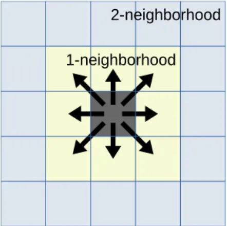
Figure 3: We call a robot’s “1-neighborhood” the eight cells directly surrounding it. At each tick, the robot can move to any of the cells in its 1-neighborhood. We call “2-neighborhood” the 16 cells directly surrounding the 1-neighborhood.

being complex to use, the main danger is for the results on exploration and mapping to be impacted by other considerations. We therefore develop a minimalistic simulator purposely built for exploration and mapping. The resulting simulator is written in Object Oriented Python, in less than 1,000 lines of code. It is composed of two main elements: the simulator which generates log files, and the Jupyter Notebook-based analysis script which extracts performance indicators from these log files and generates the graphs presented in this paper. To ensure reproducibility, we follow rigorous software development best practices. In particular, all the source code used in this paper is part of a release, and bundled together with the instructions to reproduce the log files, and re-generate the graphs. All source code is released under an open-source license1_.

The remainder of this section details the modeling used (Section 3.1), the scenarios that are run (Section 3.2), how to run a simulation (Section 3.3), what the simulator outputs (Section 3.4), and shows screenshots of the user interface (Section 3.5). Specifics about how the exploration and mapping algorithms are implemented are given in Sections 4 and 6.

3.1

Modeling

In the simulator, we represent a 2D area as a discrete number of cells. A cell is an atomic quantum of space: a single cell can either hold a single robot, be entirely filled by an obstacle, or be entirely empty. As shown in Fig. 3, a robot can move to any of the 8 cells in its 1-neighborhood. We call that movement a “step”. A robot is not constrained in the direction it moves to. That is, it can move North, then immediate South; there is no time needed to “turn its wheels”.

The simulator cuts time into discrete “ticks”. At each tick, each robot can move by one step. Multiple (possible all) robots can move during the same tick. The navigation algorithm decides, at each tick, the movement of each of the robots. It might choose to move a single robot, multiple, or all.

We assume each robot is equipped with the necessary sensors to detect the presence of an obstacle or another robot in its 1-neighborhood. These sensors allow the robot to distinguish 1 _{As an online addition to this paper, all the source code used in this paper is published under a BSD}

open-source license at [NOTE TO REVIEWERS: we’d rather not switch the repository public before the paper is published, but will do so for the camera-ready step, if accepted. It is a standalone GitHub repository. We can of course make the repository available to reviewers upon request.]. The release used in this paper is REL-1.3.

empty

canonical

floorplan

Figure 4: The three simulated scenarios. All scenario areas are the same size (80×21 cells). The starting position is depicted as a red cell on the right.

between obstacles and robots. The 1-neighborhood of a robot therefore represents the robot’s sensing range.

We further assume robots can communicate together, and can communicate back to the starting point where a central controller is located, for centralized protocols. Although our simulator does not model the constraints of the network (latency, amount of data), an Industrial IoT protocol stack such as 6TiSCH [13] seems particularly appropriate and may be considered for future work.

3.2

Scenarios

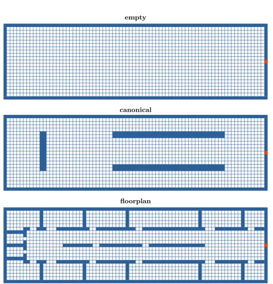
We define three scenarios to run simulations on. The term “scenario” encompasses both the location of the obstacles in the area being explored, and the location of the starting position. Fig. 4 shows the three scenarios, which we call “empty”, “canonical” and “floorplan”.

We made all three exploration areas the same size (80×21 cells) to be able to directly compare the impact of the position of obstacles on the performance of the exploration and mapping

10 Abu-Aisheh et al. algorithms. In all scenarios, all robots start from the same position (the red cell on the right wall in Fig. 4).

A scenario goes as follows. All robots are initially at the starting position which serves as a “door” into the exploration area. The goal of the algorithm is to map out that space, i.e. find which of the 630 cells are obstacles, and which are not. At the start of a simulation run, the exploration and mapping algorithm knows nothing about the area. As the robots move around in the area, they discover the position of the obstacles by moving next to them, giving the algorithm a more and more complete map. The simulation run ends when either the map completes, or when the navigation algorithm does not trigger any further robot movements. We call “completion ratio” the portion of simulation runs that result in a complete map.

We want a collection of scenarios which trigger diverse behaviors of the navigation algorithm. The “empty” scenario is the simplest one: an empty room. We use it as a reference. The “canonical” scenario is the one used extensively by Ramaithitima et al. [9]. Given that we implement Ramaithitima and compare it against other algorithm, we wanted that comparison to be done in the same conditions as in [9]. Finally, the “floorplan” scenario represents a more complete end-to-end use case, in which a swarm of robots is tasked to map out a floor of an office building. This scenario is modeled after a real office floor at Inria.

3.3

Running the Simulation

We end up implementing 4 algorithms, and have 3 scenarios. To be able to compare the impact of the number of robots, we run simulations for a number of robots ranging from 10 to 100, in steps of 10. We call a simulation cycle the resulting 4×3×10=120 simulation runs. We repeat that cycle 145 times. The full simulation time is approx. 24 h, which we split across multiple computers to speed up the simulation campaign.

Because of the random nature of some algorithms, in each of these cycles, the simulation does not execute in the same way. We end up collecting logs for 13033 simulation runs. All results are presented with a 95% confidence interval.

3.4

Simulation Outputs

Each run generates a line in a log file. This line is a JSON string that contains the following metrics:

• The “heatmap” showing how often robots have visited each of the cells. This is used to generate Fig. 8 (Section 6.1).

• The “profile”, an array that indicates the number of cells discovered at each tick. This is used to generate Fig. 9 (Section 6.2) and Fig. 10 (Section 6.3).

• The “mapping completion”, a boolean indicating whether the map is complete at the end of the exploration. This is used to generate Fig. 7 (Section 4).

3.5

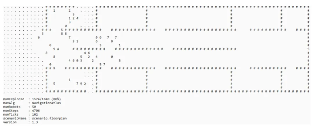
User Interface

A simple character-based user interface can be activated to see the progress of robots across the area. Fig. 5 shows a screenshot of the user interface. The user interface is deactivated by default, as it slows down the simulation. A dot (“.”) represents an unexplored cell. A hash (“#”) represents a discovered obstacle cell. An empty space (“ ”) represents a discovered open cell. Character “S” represents the start position. Numbers represent the robots.

Figure 5: User interface of the simulator.

4

Limits of Ramaithitima in Sparse Swarms

This section details preliminary simulation results for Ramaithitima. It shows that Ra-maithitima does not guarantee full exploration in sparse swarms (a small number of robots), therefore justifying the creation of the Atlas algorithm. Atlas is presented in Section 5 and its performance are examined in Section 6.

The Ramaithitima algorithm is presented in [9], and summarized in Section 2. From an implementation point of view, we implement it as a central controller. At each step of the simulation, that central controller starts by identifying the frontier robots. These are the robots which have at least one unexplored cell in their 2-neighborhood. From that set, it identifies the closest robot to the start position, and moves it to a cell further from the start position. Rather than use Euclidian distance, the controller uses the Dijkstra algorithm to compute the distance between two cells in the area, i.e. the number of steps a robot would have to take to go from one cell to the other if it took the shortest path. It repeats this process and moves as many frontier robots as possible. It then moves the non-frontier robots so they fill in the voids left by the frontier robots moving. This results in the swarm moving as a pack.

This approach works well when there is a large number of robots, as simulated in [9]. With less robots, the problem is that the frontier robots aren’t always side-by-side, so by moving each away from the starting point, it is possible to “forget” to explore an area. This is what is shown in Fig. 6: the robots progress from right to left, but pass by 2 rooms that are left unexplored. Note that this is well understood by Ramaithitima et al., which acknowledge in [9] that “The“push” strategy does not work well under such circumstances due to lack of a sufficient number of landmark robots for the bearing-based controller. [...] In the simulations presented in this letter such a situation does not arise since we use sufficient number of robots in the swarm.”. To quantify this problem, we plot in Fig. 7 the completion ratio of Ramaithitima for a number of robots between 10 and 100. The more robots, the higher the completion ratio, which is expected. Fig. 7 also shows that, the more cluttered the area, the lower the probability of creating a complete map. Yet, even with 100 robots, the completion ratio stays below 80%. Worse, regardless of the number or robots, there are always cases, even if rare, in which Ramaithitima does not result in complete exploration.

All other algorithms evaluated in this paper (including Atlas, our proposal) have a completion ratio of 100% in all cases.

12 Abu-Aisheh et al.

Ramaithitima Atlas

after 113 ticks, 30% explored after 34 ticks, 30% explored

after 205 ticks, 60% explored after 69 ticks, 60% explored

after 341 ticks, 90% explored after 108 ticks, 90% explored

Figure 6: Progress of the Ramaithitima and Atlas exploration and mapping algorithms. Using 50 robots in the floorplan scenario.

20

40

60

80

100

number of robots

0.0

0.2

0.4

0.6

0.8

1.0

ma

pp

ing

co

mp

let

ion

ra

tio

empty

canonical

floorplan

Figure 7: Completion ratio of Ramaithitima: the portion of runs where the robots map out the entire area.

5

Atlas

Atlas can be seen as an improvement of Ramaithitima to ensure mapping completion even in the extreme case of having only a single robot. It uses systematic exploration. Robots are controlled by a central controller which maintains a partial map throughout the exploration and sends robots to explore yet unexplored zones within the area. The main difference with Ramaithitima is that, instead of focusing on the frontier robots, it focuses on the frontier cells.

The central controller of Atlas does the following at each step. It starts by identifying the frontier cells, i.e. open cells which have an unexplored cell in their 1-neighborhood. From that set, it keeps only the cells which have the closest distance to the starting point. As Ramaithitima, Atlas uses topological distance (i.e. number steps along the shortest path), not Euclidian distance. Once it has the set of frontier cells and the set of robots, it identifies the robot that is closest to any frontier cell, and moves it toward the frontier cell.

The overall behavior is that the frontier expands away from the starting position, and the robots are controlled to “push” the frontier further from the starting point. In the extreme case of a single robot, that robot makes circular movements around the starting point, one step further from it at each revolution. In scenarios where there are many obstacles, the swarm can be cut into subgroups as it navigates around obstacles. This is shown in Fig. 6: the swarm starts off as one group (after 34 ticks), splits into sub-groups, each exploring separate rooms (after 69 ticks), then regroups (after 108 ticks). The full behavior of Atlas is implemented in 177 lines of code in the simulator.

6

Simulation Results

This section presents simulation results and compares the performance of four navigation and mapping algorithms: Ramaithitima, Atlas, and two random walk variants: pure random walk and ballistic random walk. In pure random walk, each robot moves to a randomly chosen open cell in its 1-neighborhood at each step. In ballistic random walk, each robot keeps moving in the same direction until it hits an obstacle or another robot. It then picks another direction at random.

6.1

Heatmaps

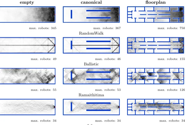
Fig. 8 allows us to qualitatively understand the behavior of the algorithms by plotting a heatmap of the number of times robots have visited each cell. With random walk, robots tend to hover around the start position, making it a very long process to explore the entire area. With ballistic, robots quickly move about the area, but because the robots are not coordinated, they tend to bounce around the same features over and over. In the Ramaithitima case, we can clearly see that some areas are visited very often, others not; it is the latter that causes Ramaithitima to sometimes “forget” to explore an area. The robot swarm in Atlas progresses from right to left; a small number splits off to explore each of the rooms. Its systematic nature makes the heatmap more homogeneous and symmetrical.

6.2

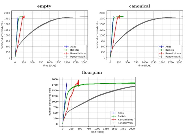
Mapping Profiles

We call mapping profile the plot that shows the number of explored cells as a function of time. It is a good representation to see the overall behavior of the algorithm. Fig. 9 shows the mapping profiles of the algorithms for each scenario.

14 Abu-Aisheh et al.

empty canonical floorplan

max. robots: 345 max. robots: 367 max. robots: 750 RandomWalk

max. robots: 49 max. robots: 46 max. robots: 155 Ballistic

max. robots: 55 max. robots: 53 max. robots: 126 Ramaithitima

max. robots: 34 max. robots: 34 max. robots: 34 Atlas

Figure 8: Heat maps of how often robots have been present on each cell, at the end of a simulation run. Results presented for a 100-robot swarm. The opacity of each cell is mapped to a different scale for each heat map; the number of robots that have passed by the darkest cell is indicated under each heat map.

empty canonical 0 250 500 750 1000 1250 1500 1750 2000 time (ticks) 0 250 500 750 1000 1250 1500 1750 2000 nu mb er disc ov ere d c ell s Atlas Ballistic Ramaithitima RandomWalk 0 250 500 750 1000 1250 1500 1750 2000 time (ticks) 0 250 500 750 1000 1250 1500 1750 2000 nu mb er disc ov ere d c ell s Atlas Ballistic Ramaithitima RandomWalk floorplan 0 250 500 750 1000 1250 1500 1750 2000 time (ticks) 0 250 500 750 1000 1250 1500 1750 2000 nu mb er disc ov ere d c ell s Atlas Ballistic Ramaithitima RandomWalk

Figure 9: Mapping profiles of the algorithms: the number of cells discovered over time. We clearly see that Random Walk explores rapidly at the very beginning (<100 ticks), then takes a very long time to discover the last unexplored cells. Ballistic, although also uncoordinated, explores the area very fast if there are no obstacles. Its performance significantly degrades in a cluttered area, such as in the floorplan case.

Ramaithitima and Atlas are coordinated, with a central controller which ensures the explo-ration is done in a systematic way. Both exhibit a mostly constant exploexplo-ration rate (a straight line in Fig. 9). In the floorplan scenario, the non-linearities of the Ramaithitima profile are because of the different rooms being explored, creating “bursts” of explored cells. We also see that the 95% confidence interval widens for Ramaithitima at the end of the exploration, as some explorations complete, others not. We can clearly see the systematic nature of Atlas, which shows a linear mapping profile throughout the exploration. This is because Atlas is designed so robots always move toward non-explored areas.

6.3

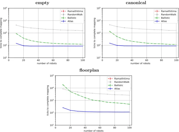
Mapping Speed

We call “mapping speed” the number of ticks from the moment the first robot enters the area until the moment the area is fully mapped. Fig. 10 plots the mapping speed as a function of the number of robots, for all algorithms and scenarios. For fair comparison, the speed (and associated 95% confidence interval) are presented only for cases where the mapping completes in all runs. No results appear for Ramaithitima as it often does not complete.

16 Abu-Aisheh et al. empty canonical 0 20 40 60 80 100 number of robots 101 102 103 104 105 tic ks to co mp let e m ap pin g Ramaithitima RandomWalk Ballistic Atlas 0 20 40 60 80 100 number of robots 101 102 103 104 105 tic ks to co mp let e m ap pin g Ramaithitima RandomWalk Ballistic Atlas floorplan 0 20 40 60 80 100 number of robots 101 102 103 104 105 tic ks to co mp let e m ap pin g Ramaithitima RandomWalk Ballistic Atlas

Figure 10: Mapping speed: time until the area is fully explored and mapped.

that a coordinated algorithm such as Atlas is significantly faster than uncoordinated algorithms (note the log scale on the y-axis). Interestingly, we see that Ballistic performs very poorly when there are many obstacles (floorplan scenario) and few robots, and they tend to enter a repetitive pattern preventing robots from quickly exploring the full area.

7

Summary and Avenues for Future Work

This paper surveys existing exploration and mapping algorithms, and proposes a taxonomy. We present an open-source simulator specifically designed for evaluating exploration and mapping algorithms. We show that existing algorithms tend to be either inefficient, or rely on dense swarms of robots. We develop Atlas, an algorithm that also produces complete maps with sparse swarms. We show by simulation that Atlas outperforms the state-of-the-art in terms of mapping accuracy and mapping speed.

This research opens up several avenues for future work. Our current simulator assumes an ideal network interconnecting the robots, yet real wireless networks suffer from limited range, limited capacity, and packet loss. Similarly, our simulator assumes perfect localization and ideal sensors. In a real system, robots don’t always know exactly where they are, and are equipped with sensors which might wrongly detect an obstacle. We are currently working on taking these constraints into account in the exploration and mapping strategy. This includes simulating continuous space and continuous time.

References

[1] S. K. Lee, S. P. Fekete, and J. McLurkin, “Structured Triangulation in Multi-Robot Systems: Coverage, Patrolling, Voronoi partitions, and Geodesic Centers,” The International Journal of Robotics Research, vol. 35, no. 10, pp. 1234–1260, 2016.

[2] J. T. Ebert, M. Gauci, and R. Nagpal, “Multi-Feature Collective Decision Making in Robot Swarms,” in 17th International Conference on Autonomous Agents and Multiagent Systems, 2018, p. 1711–1719.

[3] D. S. Drew, N. O. Lambert, C. B. Schindler, and K. S. J. Pister, “Toward Controlled Flight of the Ionocraft: A Flying Microrobot Using Electrohydrodynamic Thrust With Onboard Sensing and No Moving Parts,” IEEE Robotics and Automation Letters, vol. 3, no. 4, pp. 2807–2813, 2018.

[4] X. Huang, F. Arvin, C. West, S. Watson, and B. Lennox, “Exploration in Extreme Environ-ments with Swarm Robotic System,” in International Conference on Mechatronics (ICM), 18-20 March 2019.

[5] M. Kegeleirs, D. Garzón Ramos, and M. Birattari, “Random Walk Exploration for Swarm Mapping,” in Towards Autonomous Robotic Systems (TAROS), vol. 11650. Springer, 2019, pp. 211—-222.

[6] B. Yang, Y. Ding, Y. Jin, and K. Hao, “Self-Organized Swarm Robot for Target Search and Trapping Inspired by Bacterial Chemotaxis,” Robotics and Autonomous Systems, vol. 72, no. C, pp. 83–92, oct 2015.

[7] P. Ghassemi and S. Chowdhury, “Decentralized Informative Path Planning with Exploration-Exploitation Balance for Swarm,” in ASME International Design Engineering Technical Conferences & Computers and Information in Engineering Conference (IDETC/-CIE). ASME, 2019.

[8] G. Li, D. Zhang, and Y. Shi, “An Unknown Environment Exploration Strategy for Swarm Robotics Based on Brain Storm Optimization Algorithm,” in Congress on Evolutionary Computation (CEC). IEEE, 2019, pp. 1044–1051.

[9] R. Ramaithitima, M. Whitzer, S. Bhattacharya, and V. Kumar, “Automated Creation of Topological Maps in Unknown Environments Using a Swarm of Resource-Constrained Robots,” IEEE Robotics and Automation Letters, vol. 1, no. 2, pp. 746–753, 2016.

[10] Z. Yan, L. Fabresse, J. Laval, and N. Bouraqadi, “Metrics for Performance Benchmarking of Multi-robot Exploration,” in International Conference on Intelligent Robots and Systems (IROS), 28 Sept - 2 Oct 2015.

[11] C. Pinciroli, V. Trianni, R. O’Grady, G. Pini, A. Brutschy, M. Brambilla, N. Mathews, E. Ferrante, G. Di Caro, F. Ducatelle, M. Birattari, L. M. Gambardella, and M. Dorigo, “ARGoS: a Modular, Parallel, Multi-Engine Simulator for Multi-Robot Systems,” Swarm Intelligence, vol. 6, no. 4, pp. 271–295, 2012.

[12] R. Vaughan, “Massively Multi-robot Simulation in Stage,” Swarm Intelligence, vol. 2, pp. 189–208, 2008.

[13] X. Vilajosana, T. Watteyne, M. Vucini C, T. Chang, and K. S. J. Pister, “6TiSCH: Industrial Performance for IPv6 Internet-of-Things Networks,” Proceedings of the IEEE, vol. 107, no. 6, pp. 1153–1165, 2019.

RESEARCH CENTRE PARIS

2 rue Simone Iff - CS 42112 75589 Paris Cedex 12

Publisher Inria

Domaine de Voluceau - Rocquencourt BP 105 - 78153 Le Chesnay Cedex inria.fr