High-order accurate finite volume scheme on curved boundaries for the two-dimensional steady-state convection-diffusion equation with Dirichlet condition

(1)

HAL Id: hal-01399426

https://hal.archives-ouvertes.fr/hal-01399426

Submitted on 18 Nov 2016

HAL is a multi-disciplinary open access

archive for the deposit and dissemination of

sci-entific research documents, whether they are

pub-lished or not. The documents may come from

teaching and research institutions in France or

abroad, or from public or private research centers.

L’archive ouverte pluridisciplinaire HAL, est

destinée au dépôt et à la diffusion de documents

scientifiques de niveau recherche, publiés ou non,

émanant des établissements d’enseignement et de

recherche français ou étrangers, des laboratoires

publics ou privés.

Distributed under a Creative Commons Attribution - NoDerivatives| 4.0 International

High-order accurate finite volume scheme on curved

boundaries for the two-dimensional steady-state

convection-diffusion equation with Dirichlet condition

Ricardo Costa, Stéphane Clain, Raphaël Loubère, Gaspar Machado

To cite this version:

Ricardo Costa, Stéphane Clain, Raphaël Loubère, Gaspar Machado. High-order accurate finite volume

scheme on curved boundaries for the two-dimensional steady-state convection-diffusion equation with

Dirichlet condition. Applied Mathematical Modelling, Elsevier, 2018, 54, �10.1016/j.apm.2017.10.016�.

�hal-01399426�

(2)

High-order accurate finite volume scheme on curved boundaries for

the two-dimensional steady-state convection-diffusion equation with

Dirichlet condition

Ricardo Costaa,b, Stéphane Clainb, Raphaël Loubèrea, Gaspar J. Machadob a_{Institut de Math´}_{ematiques de Toulouse, Universit´}_{e Paul Sabatier, 31062 Toulouse, France} b_{Centro de Matem´}_{atica, Universidade do Minho, Campus de Azur´}_{em, 4800-058 Guimar˜}_{aes, Portugal}

Abstract

Accuracy may be dramatically reduced when the boundary domain is curved and numerical schemes require a specific treatment of the boundary condition to preserve the optimal order. In the finite volume context, Ollivier-Gooch and Van Altena (2002) has proposed a technique to overcome such limitation and restore the high-order accuracy which consists in specific restrictions considered in the least-squares minimization associated to the polynomial reconstruction. The method suffers of several drawbacks, particularly, the use of curved elements that requires sophisticated meshing algorithms. We propose a new method where the physical domain and the computational domain are distinct and introduce the Reconstruction of Off-site Data (ROD) where polynomial recon-struction are carried out on the mesh using data localized outside of the computational domain, namely the Dirichlet condition situated on the physical domain. A series of numerical tests assess the accuracy, convergence rates, robustness, and efficiency of the new method and show that the boundary condition is fully integrated in the scheme with a high-order accuracy and the optimal convergence rate is achieved.

Key words: High-order finite volume method, curved boundaries, Reconstruction of Off-site Data (ROD)

1. Introduction

Very high-order finite volume methods require supplemental attention to achieve the optimal order. One of the major difficulties is the boundary treatment when dealing with curved boundary domains, since polygonal meshes do not exactly fit the physical domain. Without special attention we observe a dramatic reduction of the accuracy and the method turns out to be a second-order accurate one [7, 18]. Reaching the nominal convergence order of very high-order methods then requires additional efforts and is of paramount importance nowadays [26, 28]. Several critical issues motivate the use of very high-order approximations with curved boundaries. For the Euler system, it is difficult to compute asymptotic solutions when using piecewise linear approximations of the geometries [19] even for very fine meshes. Moreover, non-physical approximations may be obtained when curved boundaries are substituted with piecewise linear straight lines [7, 18].

Several technologies to recover the optimal order have then been proposed and extensively tested. Deriving from the Finite Element approach [14, 11, 29, 30], the Discontinuous Galerkin (DG) method [12] handles curved boundaries with isoparametric elements first introduced by Bassi

(3)

and Rebay [7]. A similar approach has also been developed for the Spectral Volume (SV) method [27, 28]. In short, the technology is based on two major ingredients: the mesh considers curved elements such that the boundary of the computational domain fits with the physical boundary (at least up to a given error Ophk

q), and, the introduction of nonlinear transformations to map the curved elements to the reference one.

The method is efficient and provides optimal order of convergence but suffers of several draw-backs. The element mapping introduces the Jacobian transformations in the volume and interface integrals that we evaluate in the local basis (the reference element coordinates). Such expressions become cumbersome when dealing with high polynomial degrees and lead to an additional compu-tational effort. Moreover a change of sign of the Jacobian mapping, i.e folded or tangled elements, may occur and disqualifies the transformation [15, 16]. The second and more critical drawback is the meshing procedure with curved elements, that reveals impractical for complex geometries especially for three-dimension configurations [18]. Curved mesh generation is a today’s challenge [26] and is far from being completely solved [17]. Meshing genuinely complex geometries with unstructured hybrid grids has still not reached the level of commercial grid generators.

Alternative methods have been then proposed to avoid the nonlinear mapping and the curved mesh generation. In [18], the authors use the computational polygonal domain in place of the physical domain but modify the normal vector involved in the wall boundary condition (see also [4]). Accuracy improvement is obtained but, unfortunately, the method has only been tested with quadratic boundaries and seems to be, at most, a third-order approximation since it considers local curvature approximations, i.e. second derivatives in the Taylor expansion. Another promising method is the so-called “Extensions from Subdomains” introduced by [9, 10, 25]. The idea is to derive a new Dirichlet condition on the computational domain edge from the one evaluated on the physical boundary. An additional contribution is obtained from the integration of the solution over a path linking pointsxcompandxphyslying on their respective borders. The main advantage is that

no local mapping or curved element is required but an extension of the numerical approximation has to be evaluated in order to perform the integration of the approximation gradient outside the computational domain. Unfortunately, the method is only available for second-order operators with diffusion or viscosity term. The second drawback is the necessity to define path families between the edges of the computational mesh boundary and the physical one. Such procedure introduces constrained local minimization operations to define local one-to-one mappingsx Ñ apxq from the boundary edges and the associated pieces of the physical boundary. Then, the paths are derived from linear interpolation rx, apxqs. At last, numerical integrations over the paths are required to compute the additional contributions to update the associate Dirichlet condition on the computational boundary.

In the context of the finite volume method involving k-exact polynomial reconstructions, the pioneer work of Ollivier-Gooch and Van Altena [24] gives rise to a very high-order finite volume method dealing with curved boundary for the convection-diffusion equation and Euler and Navier-Stokes systems [21, 22, 23]. The method does not require any geometrical transformation but the mesh has to be composed with curved cells that fits the physical boundary. Likewise for the DG method, it represents a severe drawback due to the difficulties to provide such curved elements for complex geometries. Moreover, the method suffers of other problems. Indeed, one has to perform numerical integrations over the curved elements to evaluate any source term or the initial condition mean-values and on the bended boundaries to calculate the numerical fluxes. Integration on a piece of curves boundary for the two-dimensional situation requires an extra-effort for localizing the Gauss points, but, the problem turns out to be cumbersome when dealing with a three-dimensional domain

(4)

[3]. Integration over the cell is a major difficulty. Indeed, while Gaussian points are well-located for simple geometries, it seems almost impossible to derive numerical quadratures rules for generic curved element except for special situations such as pieces of circles or spheres [22].

We propose a new and simple treatment of Dirichlet conditions in the context of very high-order finite volume methods with a curved boundary domain. Because this paper is a proof of concept, we choose the simplest situation, namely the steady-state convection diffusion with Dirichlet con-dition on two-dimensional curved domain. Future extensions such as three-dimensional geometries, Neumann or mixed condition, non-stationary systems will be considered.

As in [9, 3], we consider two distinct regions: the physical domain where the continuous problem takes place and the computational polygonal domain onto which the discretization is designed and the numerical solution is evaluated. Obviously, Dirichlet conditions prescribed on the physical boundary have to be transfered in some way to the computational domain. The corner-stone of our work is the design of a specific polynomial reconstruction that takes the real boundary condition into account. Therefore we perform a reconstruction with data that are not all localized on the mesh and name the method: Reconstruction of Off-site Data (ROD) to highlight that data are not supported by the computational domain.

In some way, isoparametric element method involves two polynomials: one for the curved bound-ary and, one for the solution approximation. Conversely, the method proposed in this work uses a unique polynomial for the two associated operations Despite [3] presents some fundamental in-gredients for the polynomial reconstructions under curved boundary, the present paper proposes a simpler approach where all the integration procedures are performed on the polygonal domain.

This document is divided in seven sections. After the introduction, we formulate in section 2 the problem consider and the mesh notations, while we present the polynomial reconstructions in section 3. The fourth section is dedicated to the curved boundary where we detail the inclusion of the Dirichlet condition prescribed on the physical boundary. In section 5, the very high-order finite volume is presented and we present the numerical experiments in section 6. We end the document with the conclusions of this work.

2. Problem formulation and geometry

Let Ω be an open bounded domain of R2_{with boundary BΩ. We assume that the boundary is a}

regular Jordan curve which admits local parametrizations. We seek functionφ ” φpxq, x ” px1, x2q,

solution of the steady-state convection-diffusion equation

∇ ¨ puφ ´ κ∇φq “ f, in Ω, (1)

where u “ pu1, u2q ” pu1pxq, u2pxqq is a velocity field, κ ” κpxq is a diffusion coefficient, and

f ” f pxq is a regular source term in Ω, and where a Dirichlet condition is prescribed on the boundary BΩ with a given regular function φD” φDpxq.

A mesh M is a set of I non-overlapping convex polygonal cells ci, without gap, i P CM “

t1, . . . , Iu, and we denote by

Ω∆“

ď

iPCM

ci,

the computational domain and by BΩ∆the computational boundary associated to the mesh M. Ω∆

should be a representative domain approximation of Ω and BΩ∆ is the associated approximation

of BΩ. To this end, we assume that the nodes on BΩ∆ also belong to BΩ. We adopt the notations

(5)

• for any cell ci we denote by Bci its boundary and by |ci| its area; the reference cell point is

denoted bymi which can be any point in ci (in the present work we consider the centroid);

• two different cells ci and cj share a common edge eij whose length is denoted by |eij| and

nij “ pn1,ij, n2,ijq is the unit normal vector to eijoutward toci, i.e. nij“ ´nji; the reference

edge point ismijwhich can be any point oneij (in the present work we consider the midpoint);

if an edge ofci belongs to the boundary BΩ∆, the indexj is replaced by letter D;

• for any edge eij, we denote byqij,r,r “ 1, . . . , R, the Gaussian integration points and ζr the

associated weights;

• for any cell ci we associate the index set of neighbor cellsνpiq Ă t1, ¨ ¨ ¨ , Iu Y tDu such that

j P νpiq if eij is a common edge between cellsci andcj or with the boundary BΩ∆ ifj “ D.

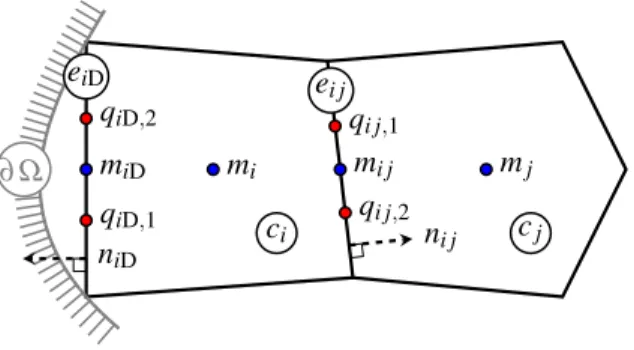
qiD,1 miD qiD,2 _q_{i j,1} mi j qi j,2 mi mj niD ci ni j cj eiD _e_{i j} ∂Ω

Figure 1: Mesh notation with edge and cell reference points (blue dots), Gauss points (red dots associated to a two-point quadrature rule), and unit normal vectors (dashed lines).

We enhance that Ω is not a polygonal domain. So, the physical domain Ω and its polygonal approximation Ω∆ do not coincide, and this usually leads to a significant accuracy degradation of

the numerical approximation.

3. Polynomial reconstruction

The polynomial reconstruction is a powerful tool to provide an accurate local representation of the underlying solution, see [1, 2] for unstructured grids and hyperbolic problems. In [8] a methodology was proposed in the context of convection-diffusion problems to achieve high accurate approximations of the gradient fluxes and take into account boundary conditions. The authors introduced different types of polynomial reconstructions namely the conservative reconstruction in cell and on boundary edge, and, the non-conservative reconstruction on inner edge, in order to compute approximations of the convective and the diffusive fluxes. In this work we mainly follows this methodology of reconstruction but apply in the specific but important case of curved boundary. 3.1. Stencil and data

A stencil is a collection of cells situated in the vicinity of a reference geometrical entity, for instance an edge or a cell, where the number of elements of the stencil shall depend on the degree d of the polynomial function we intend to construct. So, for each edge eij and cellci we associate

(6)

Remark 3.1. A polynomial reconstruction of degreed requires nd“ pd ` 1qpd ` 2q{2 coefficients in

2D. So, in practice, a stencil consists of theNd closest cells to each geometrical entity (edge or cell)

withNdě nd (we considerNd« 1.5nd for the sake of robustness).

To compute the polynomial reconstructions we need the data associated to each cell of the stencil. To this end, we assume that vector Φ “ pφiq_iPCM gathers the approximation of the mean-value of

φ over each cell, i.e.

φi« 1 |ci| ż ci φ dx. 3.2. Conservative reconstruction for cells

For each cell ci, the locald-th degree polynomial approximation of the underlying solution φ,

based on vector Φ, is defined as

φipxq “ φi`

ÿ

1ď|α|ďd

Rα

i rpx ´ miqα´ Miαs , (2)

whereα “ pα1, α2q with |α| “ α1` α2 and the conventionxα“ xα11x α2

2 . Vector Ri“ pRαiq1ď|α|ďd

gathers the polynomial coefficients, and Mα i “ |ci|1

ş

cipx ´ miq

α _{dx in order to guarantee the}

conservation property 1 |ci| ż ci φipxq dx “ φi. (3)

For a given stencilSi, we consider the quadratic functional

EipRiq “ ÿ qPSi « 1 |cq| ż cq φipxq dx ´ φq ff2 . (4)

We denote by pRi the unique vector which minimizes the quadratic functional (4) and we set pφipxq

the polynomial which corresponds to the best approximation in the least squares sense. 3.3. Non-conservative reconstruction for inner edges

For each inner edge eij, the local d-th degree polynomial approximation of the underlying

solutionφ, based on vector Φ, is defined as φijpxq “

ÿ

0ď|α|ďd

Rαijpx ´ mijqα,

where vector Rij “ pRαijq0ď|α|ďd gathers the polynomial coefficients (notice that in this case |α|

starts with 0). For a given stencil Sij with #Sij elements and vector ωij “ pωij,qqq“1,...,#Sij of

positive weights of the reconstruction, we consider the quadratic functional

EijpRijq “ ÿ qPSij ωij,q « 1 |cq| ż cq φijpxq dx ´ φq ff2 . (5)

We denote by rRij the unique vector which minimizes the quadratic functional (5) and we set rφijpxq

(7)

3.4. Conservative reconstruction for computational boundary edges

We treat the boundary edges in a particular way to take into account the prescribed Dirichlet condition. For each boundary edgeeiDon BΩ∆, the locald-th degree polynomial approximation of

the underlying solutionφ is defined as φiDpx; ψiDq “ ψiD`

ÿ

1ď|α|ďd

Rα

iDrpx ´ miDqα´ MiDαs ,

where vector RiD “ pRαiDq1ď|α|ďd gathers the polynomial coefficients, ψiD P R is a free parameter

which shall be set later, andMα

iD“ ppiD´ miDqα in order to guarantee the conservation property

ψiD“ φiDppiD;ψiDq, (6)

with piD a given collocation point. The crucial point is that piD will be a distinct point from

midpointmiD P eiD. For a given stencilSiDwith #SiDelements and vectorωiD“ pωiD,qqq“1,...,#SiD

of positive weights of the reconstruction, we consider the quadratic functional

EiDpRiDq “ ÿ qPSiD ωiD,q « 1 |cq| ż cq φiDpx; ψiDq dx ´ φq ff2 . (7)

We denote by pRiD the unique vector which minimizes the quadratic functional (7) and we set

p

φiDpx; ψiDq the polynomial which corresponds to the best approximation in the least squares sense

for the given parameterψiD and pointpiD.

Remark 3.2. The motivation for introducing the weights either for the case of a non-conservative polynomial reconstruction or for a conservative polynomial reconstruction for computational bound-ary edges is presented in [8] as well as the importance to set larger values for the adjacent cells. We refer the reader to [8] for more details.

4. Reconstructions for Off-site Data (ROD) 4.1. The Ollivier-Gooch and Van Altena method

An accurate approximation of boundary conditions on curved boundaries is of paramount im-portance when dealing with very high-order methods, since to approximate a curved boundary with a polygonal mesh generally leads to a second-order approximation [26]. The seminal paper of Ollivier-Gooch and Van Altena [24] introduces a technique for constraining the least-squares problem associated to the polynomial reconstructions on the boundary elements. Such approach requires that the reconstructed solution satisfies the boundary condition exactly at the flux inte-gration points (collocation points) [22]. In order to properly represent the boundary condition, the mesh has to fit with the physical boundary, that is, the edges of the mesh are curved for matching the real boundary (see Figure 2). As mentioned in the introduction, this approach brings several drawbacks: one has to carefully design Gauss quadrature procedures to take into account curved boundaries for preserving the accuracy [23], and, designing boundary-fitted mesh for non polygonal domain is still nowadays a difficult task [26]. In this work we avoid the difficult construction of boundary-fitted mesh, and, solely work on the easy to construct polygonal mesh.

(8)

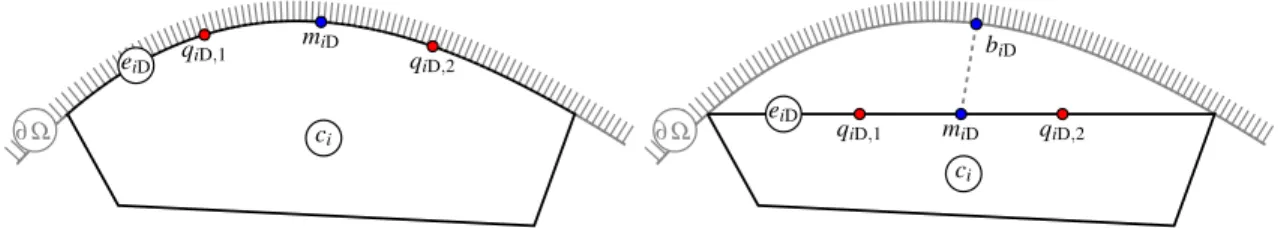
qiD,1 miD _q_iD,2 eiD ci ∂Ω qiD,1 miD qiD,2 biD eiD ci ∂Ω

Figure 2: The physical boundary BΩ and the curved boundary edge eiDwith reference points on the cell (blue dot),

Gauss points (red dots associated to a two-point quadrature rule) and the edge mid-point miD — Left: situation

when curved cells are considered — Right: situation considered in this work with straight-edge cell and an associated collocation point biDto miD.

4.2. The ROD method

We propose a different technique to prescribe Dirichlet conditions on curved boundaries.The main idea is to keep separated the computational domain from the physical one, and, perform all computations on the polygonal cells, but taking into account the information located on the physical boundary via the polynomial reconstructions. “Off-site Data” method is meant to remind that the scheme and the solutions are acting on the computational domain Ω∆, but including information

which is not associated to any geometrical entity of Ω∆(cell, edge, or point). The main advantages

are:

• numerical integration of flux or functions are only carried out on a polygonal domain and not on the complex physical domain;

• no curved elements are required, only the computational polygonal mesh is necessary; • no geometrical transformations are required involving possibly complex Jacobian functions

for the integrals;

• no Gaussian points on the physical boundary BΩ are required;

• the method design does not depend on the number of spacial dimensions.

The technique is intrinsically associated to the conservative polynomial reconstruction given in section 3.4 where, for a given edge eiD of the computational boundary BΩ∆, we define the

polynomial approximation pφiDpx; ψiDq depending on parameter ψiD and pointpiD which satisfies

the conservation property (6). We also mention thatbiDstands for a point on the physical boundary

BΩ, somewhere facing edge eiDas depicted in Figure 2-right whilemiDstands for the edge mid-point.

The Dirichlet condition will be enforced via a clever choice of the values of free parameter ψiD

and pointpiD. As a consequence one has to design a procedure to compute the free parameter such

that we simultaneously satisfy the conservation and provide a very-high order approximation of the boundary condition.

4.2.1. Second-order approximation

A simple approach consists in using piD “ miD and in setting the free parameter as ψiD “

φDpmiDq. Such a choice provides no more than a second-order convergence rate since miD does not

represent properly the physical boundary. Moreover, we need an extension of functionφD in the

(9)

4.2.2. Very high-order approximation: ROD1

In order to enforce the Dirichlet condition more accurately, we now set piD “ biD and the

free parameter ψiD “ φDpbiDq. Notice that the flux integration will nonetheless be computed on

the straight edge of the computational mesh as presented in section 5.2 and not on the physical boundary as in [24]. We expect a high-order accuracy since the reconstruction satisfies the Dirichlet condition on one point associated to the true physical boundary.

4.2.3. Very high-order approximation: ROD2

The major drawback of the method ROD1 is that the least-squares problem (7) is based on pointpiD that depends on the physical domain boundary and if the physical boundary evolves, for

instance for time dependent moving domains or interface tracking problems, one has to rebuild the whole reconstruction procedure for boundary cells/edges. We improve the previous technique by decoupling the Dirichlet condition from the interpolation problem still preserving the high-order of accuracy. We start again by setting the collocation pointpiD“ miDas in the second-order method.

Hence the least-squares procedure (7) no longer depends on the physical boundary position. Next the free parameterψiD is computed in a special way. To this end, let us introduce the functional

ψiDÑ BiDpbiD;ψiDq “ pφiDpbiD;ψiDq ´ φDpbiDq. (8)

Notice that BiD is affine with respect to ψiD. We now seek forψ˚iD as the unique solution which

satisfies the affine problem

BiDpbiD;ψiDq “ 0, (9)

the solution of which is obtained by taking two values ψ0

iD and ψ 0

iD ` 1. After some algebraic

simplifications one get ψ˚ iD“ ψ 0 iD´ BiDpbiD;ψiD0 qpψ0iD´ 1q BiDpbiD;ψ0iDq ´ BiDpbiD;ψiD0 ` 1q , (10) withψ0

iD is some real value. In other words, we adjust the free parameter on pointmiD to satisfy

the Dirichlet condition onbiD. In practice, we take ψ0iD “ φDpmiDq since ψiD˚ is supposed to be

close toφDpmiDq for regular solutions.

Remark 4.1. The methods ROD1 and ROD2 mainly differ in the structure of the matrix that compute the polynomial coefficients with respect to the data and the Dirichlet condition. In the first case, the matrix depends on the position of the point where the Dirichlet is evaluated but does not require the additional treatment given in relation (10). On the contrary, the ROD2 method provides a matrix that does not depend of the position of the Dirichlet condition but an extra-computational effort is necessary to fix the free parameter with (10). To sum-up, if one considers a fix curved domain, the ROD1 method is more efficient whereas the ROD2 technique is well-adapted to situations where the physical boundary changes with the time or during an iterative process. Remark 4.2. The coefficients pRiDof the polynomial function pφiDpx; ψiDq are obtained as the

matrix-vector product between the Moore-Penrose matrix associated to the least-square problem and the vector of cell values in the stencil [8]. The matrix structure does not depend on the physical boundary position by construction but only depends on the computational mesh. The Dirichlet condition is only prescribed via functional (8) and satisfies condition (9).

(10)

5. High-order finite volume scheme 5.1. Generic finite volume scheme

To obtain a finite volume scheme, equation (1) is integrated over each cellci and applying the

divergence theorem we get ż Bci puφ ´ κ∇φq ¨ nids “ ż ci f dx, (11)

where Bci is the cell boundary and ni is the associated outward unit vector. Considering the

Gaussian quadrature with_{R P N}˚ _{points for the line integrals, i.e. of order 2}_{R, we get the residual}

expression ÿ jPνpiq |eij| « _R ÿ r“1 ζr ` FCij,r` F D ij,r ˘ ff ´ fi|ci| “ Oph2Ri q, (12)

with the physical fluxes given by

FCij,r“ upqij,rq ¨ nijφpqij,rq and FDij,r“ ´κpqij,rq∇φpqij,rq ¨ nij,

and withhi “ maxjPνpiq|eij|, while fi stands for an approximation of order 2R of the mean value

off over cell ci. Notice that if cell ci is not triangular, we split it into sub-triangles which share

the cell centroid as a common vertex and apply the quadrature rule on each sub-triangle as in [13]. Using the different polynomial reconstructions see previous sections, we design the numerical scheme with two main ingredients: the flux computation and the solver. We use a similar technique proposed in [8, 3], particularly the matrix-free approach is adopted, based on the residual operator construction.

5.2. Numerical fluxes

Numerical fluxes are computed with respect to the edges:

• for the inner edges eij, the fluxes at the quadrature pointqij,r write

FC

ij,r “ rupqij,rq ¨ nijs`φp_ipq_ij,rq ` rupq_ij,rq ¨ n_ijs´φp_jpq_ij,rq, FD

ij,r “ ´κpqij,rq∇ rφijpqij,rq ¨ nij;

• for the boundary edges eiD, the fluxes at the quadrature pointqiD,r write

FC

iD,r“ rupqiD,rq ¨ niDs`φpipqiD,rq ` rupqiD,rq ¨ niDs´φpiDpqiD,rq,

FiD,rD “ ´κpqiD,rq∇ pφiDpqiD,rq ¨ niD.

Notice that all the fluxes are computed on the edges of the computational domain without any reference to the physical domain. The Dirichlet condition on BΩ is implicitly contained in the polynomial reconstructed function pφiD.

(11)

5.3. Residual operator and solver

For any vector Φ in RI_{, we define the residual operators for cells}_c

i,i “ 1, . . . , I, as GipΦq “ ÿ jPνpiq |eij| « _R ÿ r“1 ζr`Fij,rC ` F D ij,r ˘ ff ´ fi|ci|, (13)

which corresponds to the finite volume scheme (12) cast in residual form. Gathering all the com-ponents of the residuals provides a global affine operator GpΦq “ pGipΦqq_iPCM and we seek vector

Φ‹

P RI, solution of the problem GpΦq “ 0. The GMRES method, powered by a preconditioning matrix, is carried out to compute an approximation of Φ‹ _{as in [8, 3].}

6. Numerical results

In order to validate the implementation of the methods and assess the accuracy and the con-vergence rates, we manufacture several analytical solutions on specific domains which require the computation of an associated source term to satisfy equation (1). Vector Φ‹ _{“ pφ}‹

iqiPCM gathers

the numerical approximations of the mean values ofφ while vector Φ “ pφiqiPCM gathers the exact

mean valuesφi ofφ, that is φi“ p1{|ci|q

ş

ciφ dx.

The normalizedL1_{- and}_L8_{-norm errors, denoted by}_E

1 andE8, are computed respectively as

E1pMq “ ÿ iPCM |φ‹i ´ φi||ci| ÿ iPCM |φi||ci| and E8pMq “ max iPCM|φ ‹ i ´ φi| ÿ iPCM |φi||ci| .

The convergence rate for the normalizedL1_{- and}_L8_{-norm errors between two different meshes}

M1 and M2, with DOF1 and DOF2 degrees of freedom, respectively, where DOF1 ‰ DOF2, is

evaluated as

OαpM1, M2q “ 2

| logpEαpM1q{EαpM2qq|

| logpDOF1{DOF2q|

, α P t1, 8u.

In all the simulations, the weights in functionals (5) and (7) are set toωij,q “ 3, i P CM, j P νpiq,

q P Sij, ifeij is an edge ofcq andωij,q “ 1, otherwise.

For the sake of simplicity, we name the method given in section 4.2.1 as “second-order method”, the one given in section 4.2.2 as “ROD1 method”, and the proposed method, presented in section 4.2.3, as “ROD2 method”. The methodology of validation consists in observing the rates of con-vergence under mesh refinement when high-order polynomial reconstructions (Pk, k “ 1, 3, 5) are

employed for different strategies dealing with Dirichlet boundary conditions defined on the physical curved domains. Only smooth solutions of the steady-state two-dimensional convection-diffusion equation are considered. The different curved physical domains are

• An annulus domain in section 6.1. We simulate with triangular (possibly refined) grids low P´eclet number, high P´eclet number and pure convection problems.

• A rose-shaped domain in section 6.2. A deformation of the annulus permits to define branches on the interior and exterior boundaries. We simulation with triangular and quadrangular grids two cases, a rose with three-three branches and a five-three rose both.

(12)

6.1. Annulus domain

In this first set of numerical tests we consider an annulus domain with center at p0, 0q charac-terized by the interior and exterior circumferences ΓIand ΓE, respectively with radiusrI“ 0.5 and

rE “ 1. For the convection-diffusion problem (1), we prescribe a constant radial velocity u and

κ “ 1. We then seek for a manufactured solution, invariant by rotation, given be φpx1, x2q “ a`exppur1q ` expp´ur1q ` b˘ , r1” r1prq “

p2r ´ prE` rIqq

prE´ rIq

, withr2

“ x21` x22 such thatr1 P r´1, 1s. We also prescribe homogeneous Dirichlet conditions on

the two boundaries ΓI and ΓE and deduce that b “ ´ exppuq ´ expp´uq while a “ 1{pexppuq `

expp´uq ´ 2q guarantees the property φ P r´1, 0s in Ω. The associated source term f is obtained after substituting the solution into equation (1).

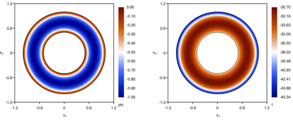
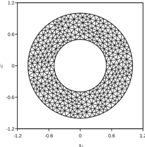
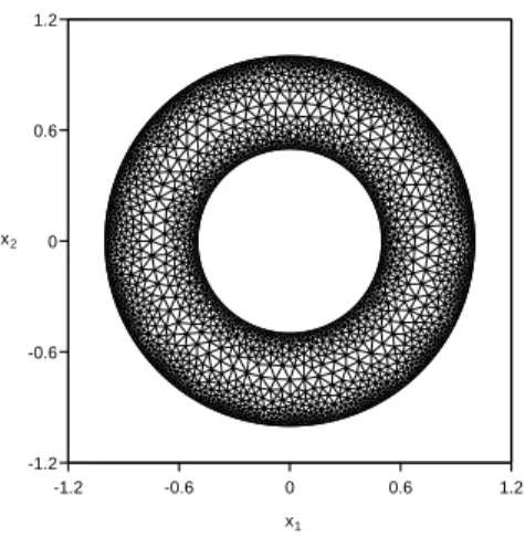
Low P´eclet number. We first address the low P´eclet number situation setting u “ 1. We plot in Figure 3 the manufactured solution and the source term. The simulations were carried out with successive refined uniform triangular Delaunay meshes (see Figure 4). Observe that boundary vertices belong to the true physical domain boundary.

(13)

-1.2 -0.6 0 0.6 1.2 -1.2 -0.6 0 0.6 1.2 1 x2 x

Figure 4: Coarse uniform triangular Delaunay mesh prescribed for the annulus domain.

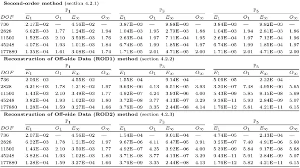
We report in Table 1 the errors and the convergence rates for the second-order, and the two ROD methods. The second-order approach provides at most a second-order convergence for both error norms, whatever the degree of the polynomial reconstruction. These results are expected since the Dirichlet condition is affected with a mismatch of order Oph2

q due to the erroneous location with respect to the physical boundary. The two other methods recover the optimal order and achieve an effective second-, fourth-, and sixth-order convergence rates for P1, P3, and P5 polynomial

reconstructions, respectively, while no oscillations are reported. The accuracy of both methods are quite comparable and clearly overcome the second-order limitation expected when dealing with the curved boundary with non-fitted cells.

(14)

Table 1: Annulus problem for low P´eclet number — Errors and convergence rates for the second-order, the ROD1 and ROD2 methods with uniform triangular Delaunay meshes.

Second-order method (section 4.2.1)

P1 P3 P5

DOF E1 O1 E8 O8 E1 O1 E8 O8 E1 O1 E8 O8

736 2.17E´02 — 4.56E´02 — 3.87E´03 — 9.88E´03 — 3.84E´03 — 9.82E´03 —

2828 6.62E´03 1.77 1.24E´02 1.94 1.04E´03 1.95 2.79E´03 1.88 1.04E´03 1.94 2.81E´03 1.86

11500 1.52E´03 2.10 3.59E´03 1.76 2.63E´04 1.97 7.11E´04 1.95 2.63E´04 1.97 7.12E´04 1.96

45248 4.07E´04 1.93 1.01E´03 1.84 6.74E´05 1.99 1.85E´04 1.97 6.74E´05 1.99 1.85E´04 1.97

177880 1.35E´04 1.61 3.08E´04 1.74 1.71E´05 2.01 4.71E´05 2.00 1.71E´05 2.01 4.71E´05 2.00

Reconstruction of Off-side Data (ROD1) method (section 4.2.2)

P1 P3 P5

736 2.06E´02 — 4.55E´02 — 1.55E´04 — 9.14E´04 — 5.06E´05 — 2.22E´04 —

2828 6.21E´03 1.78 1.21E´02 1.97 9.63E´06 4.13 6.51E´05 3.93 3.30E´07 7.48 4.95E´06 5.65

11500 1.43E´03 2.10 3.49E´03 1.77 4.92E´07 4.24 3.93E´06 4.00 5.43E´09 5.85 9.15E´08 5.69

45248 3.82E´04 1.93 1.02E´03 1.80 3.72E´08 3.77 4.13E´07 3.29 9.38E´11 5.93 2.84E´09 5.07

177880 1.28E´04 1.59 3.27E´04 1.66 3.76E´09 3.35 2.44E´08 4.14 1.76E´12 5.81 4.21E´11 6.15

P1 P3 P5

736 2.07E´02 — 4.56E´02 — 1.54E´04 — 9.01E´04 — 4.74E´05 — 2.13E´04 —

2828 6.22E´03 1.78 1.21E´02 1.97 9.67E´06 4.11 6.47E´05 3.91 3.25E´07 7.40 4.91E´06 5.60

11500 1.43E´03 2.10 3.50E´03 1.77 4.92E´07 4.25 3.92E´06 4.00 5.39E´09 5.84 9.17E´08 5.68

45248 3.82E´04 1.93 1.02E´03 1.80 3.71E´08 3.77 4.13E´07 3.29 9.43E´11 5.91 2.84E´09 5.07

177880 1.28E´04 1.59 3.27E´04 1.66 3.76E´09 3.35 2.44E´08 4.13 1.76E´12 5.82 4.21E´11 6.15

High P´eclet number. Large P´eclet number is prescribed taking u “ 10 and we plot in Figure 5 the manufactured solution and the source term. This test addresses the scheme robustness and accuracy to preserve the boundary condition when dealing with small boundary layers with respect to the dimension of the whole geometry. The simulations were carried out with successive refined Delaunay meshes plotted in Figure 6 where, again, the boundary vertices belong to the physical boundary.The meshes are refined close to the boundaries to better capture the boundary layers.

(15)

-1.2 -0.6 0 0.6 1.2 -1.2 -0.6 0 0.6 1.2 1 x2 x

Figure 6: Coarse non-uniform triangular Delaunay mesh prescribed for the annulus domain for the high P´eclet number test case.

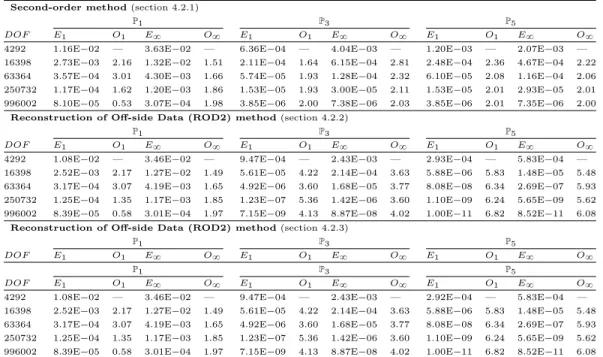
In Table 2, we report the errors and the convergence rates for the three methods. As for the low P´eclet problem the second-order method reaches at most a second-order convergence for both error norms while the two ROD methods achieve an effective second-, fourth-, and sixth-order convergence rates for P1, P3, and P5polynomial reconstructions, respectively. We conclude that the

high-order methods effectively handle large P´eclet number situations achieving optimal convergence rates without any oscillation.

(16)

Table 2: Annulus problem for high P´eclet number — Errors and convergence rates for the second-order and the two ROD methods with adapted triangular Delaunay meshes.

P1 P3 P5

4292 1.16E´02 — 3.63E´02 — 6.36E´04 — 4.04E´03 — 1.20E´03 — 2.07E´03 —

16398 2.73E´03 2.16 1.32E´02 1.51 2.11E´04 1.64 6.15E´04 2.81 2.48E´04 2.36 4.67E´04 2.22

63364 3.57E´04 3.01 4.30E´03 1.66 5.74E´05 1.93 1.28E´04 2.32 6.10E´05 2.08 1.16E´04 2.06

250732 1.17E´04 1.62 1.20E´03 1.86 1.53E´05 1.93 3.00E´05 2.11 1.53E´05 2.01 2.93E´05 2.01

996002 8.10E´05 0.53 3.07E´04 1.98 3.85E´06 2.00 7.38E´06 2.03 3.85E´06 2.01 7.35E´06 2.00

P1 P3 P5

4292 1.08E´02 — 3.46E´02 — 9.47E´04 — 2.43E´03 — 2.93E´04 — 5.83E´04 —

16398 2.52E´03 2.17 1.27E´02 1.49 5.61E´05 4.22 2.14E´04 3.63 5.88E´06 5.83 1.48E´05 5.48

63364 3.17E´04 3.07 4.19E´03 1.65 4.92E´06 3.60 1.68E´05 3.77 8.08E´08 6.34 2.69E´07 5.93

250732 1.25E´04 1.35 1.17E´03 1.85 1.23E´07 5.36 1.42E´06 3.60 1.10E´09 6.24 5.65E´09 5.62

996002 8.39E´05 0.58 3.01E´04 1.97 7.15E´09 4.13 8.87E´08 4.02 1.00E´11 6.82 8.52E´11 6.08

P1 P3 P5

4292 1.08E´02 — 3.46E´02 — 9.47E´04 — 2.43E´03 — 2.92E´04 — 5.83E´04 —

16398 2.52E´03 2.17 1.27E´02 1.49 5.61E´05 4.22 2.14E´04 3.63 5.88E´06 5.83 1.48E´05 5.48

63364 3.17E´04 3.07 4.19E´03 1.65 4.92E´06 3.60 1.68E´05 3.77 8.08E´08 6.34 2.69E´07 5.93

250732 1.25E´04 1.35 1.17E´03 1.85 1.23E´07 5.36 1.42E´06 3.60 1.10E´09 6.24 5.65E´09 5.62

996002 8.39E´05 0.58 3.01E´04 1.97 7.15E´09 4.13 8.87E´08 4.02 1.00E´11 6.82 8.52E´11 6.08

Pure convection. We address the pure convection situation setting κ “ 0 and u “ 1 and plot in Figure 7 the manufactured solution and the source term. The simulations were carried out with successive refined uniform triangular Delaunay meshes presented in Figure 4 and, as in the previous tests, the boundary vertices belong to the boundary curves.

Figure 7: Manufactured solution (left panel) and source term (right panel) for the pure convection test case.

We report in Table 3, the errors and the convergence rates for the three methods. As in the previous situations, the second-order boundary approach is doomed to a second-order of accuracy

(17)

while the two other methods efficiently handle the convection problem with curved boundaries with no oscillations and no artificial diffusion.

Table 3: Annulus problem for pure convection — Errors and convergence rates for the second-order and the ROD methods with uniform triangular Delaunay meshes.

P1 P3 P5

736 1.01E´02 — 4.43E´02 — 6.78E´03 — 1.07E´02 — 6.88E´03 — 1.01E´02 —

2828 3.62E´03 1.52 2.35E´02 0.94 1.92E´03 1.88 2.92E´03 1.93 1.93E´03 1.89 2.85E´03 1.88

11500 8.67E´04 2.04 1.07E´02 1.12 4.81E´04 1.97 7.19E´04 2.00 4.82E´04 1.98 7.18E´04 1.97

45248 2.23E´04 1.98 1.91E´03 2.51 1.24E´04 1.98 1.86E´04 1.98 1.24E´04 1.98 1.86E´04 1.98

177880 6.85E´05 1.72 4.07E´03 1.11 3.15E´05 2.00 4.72E´05 2.00 3.15E´05 2.00 4.72E´05 2.00

P1 P3 P5

736 8.75E´03 — 3.87E´02 — 2.35E´04 — 1.26E´03 — 3.48E´05 — 1.32E´04 —

2828 3.45E´03 1.38 2.15E´02 0.87 2.47E´05 3.35 1.09E´04 3.63 1.25E´06 4.95 5.26E´06 4.79

11500 8.07E´04 2.07 1.03E´02 1.05 1.58E´06 3.91 9.50E´06 3.48 2.34E´08 5.67 1.14E´07 5.46

45248 2.06E´04 2.00 1.81E´03 2.54 1.21E´07 3.76 8.04E´07 3.61 5.04E´10 5.60 3.11E´09 5.26

177880 6.49E´05 1.69 4.05E´03 1.17 8.45E´09 3.89 9.60E´08 3.10 8.65E´12 5.94 5.76E´11 5.83

P1 P3 P5

736 8.75E´03 — 3.87E´02 — 2.36E´04 — 1.26E´03 — 3.57E´05 — 1.33E´04 —

2828 3.45E´03 1.38 2.15E´02 0.87 2.47E´05 3.35 1.10E´04 3.63 1.25E´06 4.98 5.27E´06 4.80

11500 8.07E´04 2.07 1.03E´02 1.05 1.59E´06 3.91 9.50E´06 3.49 2.34E´08 5.68 1.14E´07 5.47

45248 2.06E´04 2.00 1.81E´03 2.54 1.21E´07 3.76 8.04E´07 3.61 5.04E´10 5.60 3.11E´09 5.26

177880 6.49E´05 1.69 4.05E´03 1.17 8.45E´09 3.89 9.61E´08 3.10 8.64E´12 5.94 5.76E´11 5.83

6.2. Rose-shaped domain

We now consider a more complex geometry where the annulus is transformed by a diffeomor-phism mapping which consists in a periodic transformation of the boundaries in the following way:

ΓI :„x1 x2  “ RIpθ; αIq„cospθq sinpθq  and ΓE:„x1 x2  “ REpθ; αEq„cospθq sinpθq  , where pr, θq are the polar coordinates and RIpθ; αIq and REpθ; αEq, αI, αEP R, are given by

RIpθ; αIq “ rI ˆ 1 ` 1 10sinpαIθq ˙ and REpθ; αEq “ rE ˆ 1 ` 1 10sinpαEθq ˙ . The global mapping from the Rose-shaped domain onto the annulus then reads

„y1 y2  Ñ„x1 x2  “ T py1, y2q “ ˆ RE´ r RE´ RI RIpθ; αIq ` r ´ RI RE´ RI REpθ; αEq˙ „cospθq sinpθq  . The manufactured solution on the Rose-shaped domain is then given by

ψpx1, x2q “ φpT´1px1, x2qq.

Notice that we recover the annulus geometry withαI “ αE “ 0. The associated source term f is

obtained from equation (1) while homogeneous Dirichlet boundary condition still holds on the new boundaries ΓI and ΓE. All the simulations have been carried out withκ “ 1 and u “ 1

(18)

First test. The transformation is parametrized withαI “ 3 and αE “ 3 and we plot in Figure 8

the manufactured solution and the source term in the new domain.

Figure 8: Manufactured solution (left panel) and source term (right panel).

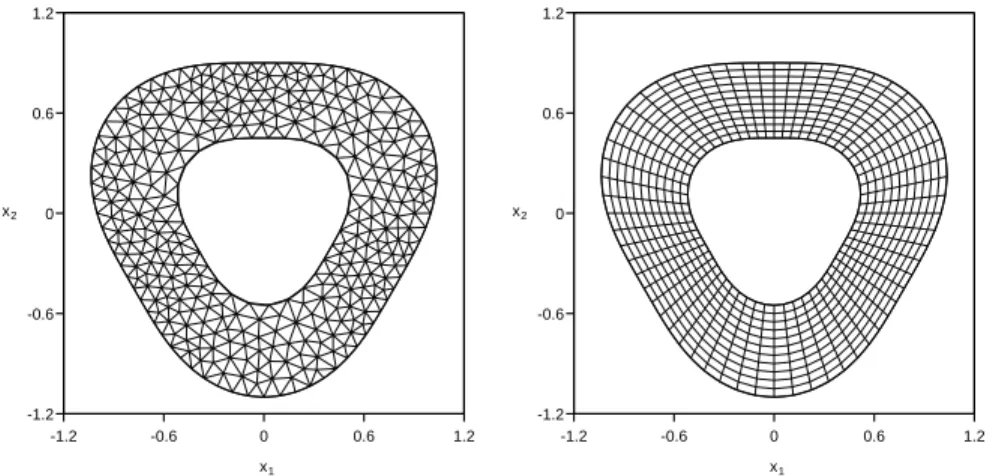
We carried out the simulations with successive refined regular triangular Delaunay meshes and also with quadrilateral meshes, see Figure 9, to show the ability of the method to handle different cell shapes. -1.2 -0.6 0 0.6 1.2 -1.2 -0.6 0 0.6 1.2 x 2 x 1 -1.2 -0.6 0 0.6 1.2 -1.2 -0.6 0 0.6 1.2 2 1 x x

Figure 9: Coarse uniform triangular Delaunay mesh (left panel) and uniform quadrilateral mesh (right panel) pre-scribed for the rose-shaped domain.

We report in Table 4 the errors and the convergence rates obtained with the ROD2 method (Delaunay meshes) while Table 5 reports the same informations for the quadrangular meshes. We obtain the optimal convergence orders and no oscillation is reported. Computations have also been carried out with the second-order boundary approximation (not presented here) and we observe a second-order of convergence due to an inadequate treatment of the boundary condition.

(19)

Table 4: Rose-shaped problem — Test 1 — Errors and convergence rates for the ROD method with uniform triangular Delaunay meshes.

P1 P3 P5

667 2.21E´02 — 4.91E´02 — 3.59E´04 — 3.56E´03 — 2.20E´04 — 1.52E´03 —

2590 6.23E´03 1.86 1.40E´02 1.85 1.85E´05 4.38 2.30E´04 4.04 2.77E´06 6.45 3.04E´05 5.77

10274 1.48E´03 2.09 4.49E´03 1.65 1.17E´06 4.00 2.02E´05 3.53 5.58E´08 5.67 1.12E´06 4.79

41367 3.29E´04 2.16 1.21E´03 1.88 9.17E´08 3.66 1.53E´06 3.71 7.02E´10 6.28 2.07E´08 5.73

165599 6.96E´05 2.24 3.45E´04 1.81 6.58E´09 3.80 1.07E´07 3.83 1.37E´11 5.68 3.85E´10 5.74

Table 5: Rose-shaped problem — Test 1 — Errors and convergence rates for the ROD2 method with uniform quadrilateral meshes.

P1 P3 P5

660 6.42E´02 — 8.73E´02 — 1.41E´03 — 7.86E´03 — 9.75E´04 — 4.73E´03 —

2760 1.61E´02 1.93 2.23E´02 1.91 2.56E´04 2.39 8.45E´04 3.12 1.20E´05 6.15 8.33E´05 5.65

11280 4.02E´03 1.97 5.60E´03 1.96 2.00E´05 3.62 8.48E´05 3.27 1.66E´07 6.08 1.08E´06 6.17

46080 9.87E´04 2.00 1.38E´03 1.99 1.14E´06 4.07 5.93E´06 3.78 2.76E´09 5.83 2.00E´08 5.68

185280 2.47E´04 1.99 3.45E´04 1.99 7.50E´08 3.91 3.84E´07 3.93 7.72E´11 5.14 3.42E´10 5.85

Second test. The second test deals with a more wavy boundary settingαI “ 3 and αE “ 5. We

plot in Figure 10 the manufactured solution and the source term.

Figure 10: Manufactured solution (left panel) and source term (right panel).

As in the previous case, simulations with successive refined regular Delaunay meshes or quadri-lateral meshes have been carried out, see Figure 11.

(20)

-0.6 0 0.6 0 0.6 1.2 1.2 -1.2 -1.2 -0.6 x x1 2 -1.2 -0.6 0 0.6 1.2 -1.2 -0.6 0 0.6 1.2 2 1 x x

Figure 11: Coarse uniform triangular Delaunay mesh (left panel) and uniform quadrilateral mesh (right panel) prescribed for the rose-shaped domain.

We report in Tables 6 and 7 the errors and the convergence rates obtained with the ROD2 method and confirm the ability of the scheme to preserve the optimal order in function of the polynomial degree used for the reconstruction procedure.

Table 6: Rose-shaped problem — Test 2 — Errors and convergence rates for the ROD method with uniform triangular Delaunay meshes.

P1 P3 P5

645 2.71E´02 — 6.97E´02 — 6.80E´04 — 8.76E´03 — 5.12E´04 — 5.86E´03 —

2550 7.56E´03 1.86 2.30E´02 1.61 4.49E´05 3.95 7.62E´04 3.55 1.29E´05 5.36 2.45E´04 4.62

10244 1.89E´03 2.00 7.30E´03 1.65 3.71E´06 3.59 1.28E´04 2.57 2.98E´07 5.42 1.39E´05 4.12

40789 4.10E´04 2.21 1.97E´03 1.89 2.53E´07 3.89 6.70E´06 4.27 9.53E´09 4.98 4.91E´07 4.84

162011 9.63E´05 2.10 5.92E´04 1.75 1.89E´08 3.76 9.37E´07 2.85 1.20E´10 6.34 1.07E´08 5.55

Table 7: Rose-shaped problem — Test 2 — Errors and convergence rates for the ROD2 method with uniform quadrilateral meshes.

P1 P3 P5

660 6.91E´02 — 1.11E´01 — 5.06E´03 — 3.27E´02 — 5.37E´03 — 3.60E´02 —

2760 1.74E´02 1.93 2.85E´02 1.90 3.94E´04 3.57 3.57E´03 3.10 1.33E´04 5.17 1.61E´03 4.35

11280 4.37E´03 1.96 7.13E´03 1.97 4.70E´05 3.02 3.83E´04 3.17 2.27E´06 5.78 5.07E´05 4.91

46080 1.08E´03 1.99 1.77E´03 1.98 3.36E´06 3.75 2.50E´05 3.88 4.85E´08 5.47 1.07E´06 5.48

185280 2.71E´04 1.99 4.42E´04 1.99 2.05E´07 4.02 1.57E´06 3.98 1.11E´09 5.42 1.41E´08 6.22

7. Conclusions

We have presented a high-order finite volume scheme to solve the steady-state bi-dimensional convection-diffusion problem based on a new class of polynomial reconstructions. Two approaches were proposed to overcome the second-order accuracy limitation when dealing with non polyg-onal domain and Dirichlet boundary conditions. The first one consists in analytically constrain

(21)

the boundary element reconstructions in order to satisfy the boundary condition at a point on the physical domain boundary. Such approach differs from the Olliver-Gooch and Van Altena approach in the sense that the flux calculation is performed on the straight edge and no curved element is necessary. The proposed ROD method consists in constraining the boundary reconstructions by a posteriori computing the associated free parameter such that the reconstructions satisfy appro-priately the boundary condition. This procedure relies on the fact that the least-squares matrix associated to the reconstruction is decoupled from the boundary parameterization and, therefore, is less sensitive to the boundary location.

Several numerical tests considering simple and complex curved domains were simulated to ob-serve that we achieve effective optimal order of accuracy both for structured and unstructured meshes for the two-dimensional linear steady-state convection-diffusion problem. A pure convec-tion problem (hyperbolic scalar equaconvec-tion) was also tested and optimal order accuracy rates were achieved without any reported oscillation.

This work represents a proof of concept showing that very high-order of accuracy Finite Volume scheme on unstructured can handle curved boundary conditions at the optimal order of accuracy without the need for a boundary fitted mesh or complex transformations. For future works we plan to extend this approach to other boundary conditions (Neumann, Robin), to unsteady systems (Euler, Navier-Stokes) with time evolving domain (piston, pulsating interfaces, etc.). We also plan to investigate the extension of ROD to unstructured 3D mesh. Even if, conceptually speaking, the ROD method does not depend on the space dimension, the machinery needed in three-dimensional will demand delicate validation and verification.

Acknowledgements

This research was financed by FEDER Funds through Programa Operational Fatores de Compet-itividade — COMPETE and by Portuguese Funds FCT — Funda¸c˜ao para a Ciˆencia e a Tecnologia, within the Strategic Project UID/MAT/00013/2013.

R. L. and R. C. thank the financial support of the “International Centre for Mathematics and Computer Science in Toulouse” (CIMI) partially supported by ANR-11-LABX-0040-CIMI within the program ANR-11-IDEX-0002-02.

References References

[1] T.J. Barth, P.O. Frederickson, Higher order solution of the Euler equations on unstructured grids using quadratic reconstruction, AIAA Paper 90-0013, 1990.

[2] T.J. Barth, Recent developments in high order k-exact reconstruction on unstructured meshes, AIAA Paper 93-0668, 1993.

[3] A. Boularas, S. Clain, F. Baudoin, A sixth-order finite volume method for dif-fusion problem with curved boundaries, Applied Mathematical Modelling, 41 (2017) http://dx.doi.org/10.1016/j.apm.2016.10.004

[4] N. Balakrishnan and G. Fernandez, Wall boundary conditions for inviscid compressible flows on unstructured meshes, Int. J. Numer. Meth. Fluids 28 (1998) 1481–1501.

(22)

[5] F. Bassi, S. Rebay, High-order accurate discontinuous solution of the 2D Euler equations, Jour-nal of ComputatioJour-nal Physics, 138 (2) (1997), pp. 251–285.

[6] B. Baghapour, V. Esfahanian, A. Nejat, A Framework for Curved Boundary Representation in 2D Discontinuous Galerkin Euler Solvers, Journal of Applied Fluid Mechanics, 7(4) (2014) 693–702.

[7] F. Bassi, S. Rebay, High-order accurate discontinuous finite element solution of the 2D Euler equations, J. Comput. Phys. 138 (2) (1997) 251285,

[8] S. Clain, G. J. Machado, J. M. N´obrega, R. M. S. Pereira, A sixth-order finite volume method for the convection-diffusion problem with discontinuous coefficients, Computer Methods in Applied Mechanics and Engineering 267 (2013) 43–64.

[9] B. Cockburn, M. Solano, Solving Dirichlet boundary-value problems on curved domains by extensions from subdomains, SIAM J. Sci. Comput. 34 (2012) 497–519.

[10] B. Cockburn, M. Solano, Solving Convection-Diffusion Problems on Curved Domains by Ex-tensions from Subdomains J Sci Comput 59 (2014) 512–543.

[11] P. G. Ciarlet and P.A. Raviart, Interpolation over curved elements, with applications to finite element methods, Corn- put. Methods Appl. Mech. Engrg. 1 (1972), 217-249.

[12] B. Cockburn, G. E. Karniadakis, C.-W. Shu, Discontinuous Galerkin Methods, Lecture Notes in Computational Science and Engineering, Springer, 2000.

[13] A. Ern, J.-L. Guermond, Theory and Practice of Finite Elements, vol. 159, Springer Verlag, New-York, 2004.

[14] I. Ergatoudis, B. M. Irons, O. C. Zienkiewicz, Curved, isoparametric, ”quadrilateral” elements for finite element analysis, Int. J. Solids Structures, 4 (1968) 31–42.

[15] W.J. Gordon, C.A. Hall, Construction of curvilinear co-ordinate systems and applications to mesh generation, International Journal for Numerical Methods in Engineering 7(4) (1973) 461– 477.

[16] W.J. Gordon, C.A. Hall, Transfinite element methods: Blending-function interpolation over arbitrary curved element domains, Numerische Mathematik 21(2) (1973) 109–129.

[17] Geuzaine and J.-F. Remacle, Gmsh: a three-dimensional Finite Element mesh generator with built-in pre- and post-processing facilities, International Journal for Numerical Methods in En-gineering, 79 (2009) 1309–1331.

[18] L. Krivodonova, M. Berger High-order accurate implementation of solid wall boundary condi-tions in curved geometries J. Comput. Phys. 211 (2006) 492512

[19] D. J. Mavriplis, Results from the 3rd drag prediction workshop using the NSU3D unstructured mesh solver, AIAA Paper 2007-256, 2007.

[20] D. Mavriplis, N. C., K. Shahbazi, L. Wang, and N. Burgess, Progress high-order discontinuous Galerkin methods for aerospace applications, AIAA Aerospace SciencesMeeting Including The New Horizons Forum and Aerospace Exposition, 601, 2009.

(23)

[21] C. Michalak, C. Ollivier-Gooch, Unstructured high-order accurate finite volume solutions of the Navier-Stokes equations 47th AIAA Aerospace Sciences Meeting, AIAA 2009-954, 5-8 January 2009, Orlando, Florida

[22] C. Ollivier-Gooch, A. Nejat, and C. Michalak, On Obtaining High-Order Finite-Volume So-lutions to the Euler Equations on Unstructured Meshes, 18th AIAA Computational Fluid Dy-namics Conference, AIAA 2007-4464, 25-28 june 2007, Miami FL

[23] C. Ollivier-Gooch, A. Nejat, and C. Michalak, On Obtaining and Verifying High-Order Un-structured Finite Volume Solutions to the Euler Equations, AIAA Journal, 47(9) (2009), 2105– 2120.

[24] C. Ollivier-Gooch, M. Van Altena, A high-order-accurate unstructured mesh finite-volume scheme for the advection-diffusion equation, J. Comput. Phys. 181(2) (2002) 729–752.

[25] W. Qiu, M. Solano, P. Vega, A High Order HDG Method for Curved-Interface Problems Via Approximations from Straight Triangulations, J. Sci. Comput. 69 (2016) 1384–1407.

[26] Z. J. Wang, High-order computational fluid dynamics tools for aircraft design, Phil. Trans. R. Soc. A (2014) 372, 20130318.

[27] Z.J. Wang, Yen Liu, Extension of the spectral volume method to high-order boundary repre-sentation J. Comput. Phys. 211 (2006) 154–178.

[28] Z. Wang. High-order methods for the Euler and Navier-Stokes equations on unstructured grids. Progress in Aerospace Sciences, 43(13):1–41, 2007.

[29] M. Zl´amal, Curved elements in the finite element method. I, SIAM J. Numer. Anal. 10 (1973), 229-240.

[30] M. Zl´amal, Curved elements in the finite element method. II, SIAM J. Numer. Anal. 11 (1974), 347–368.