Composable inference metaprogramming using subproblems

Composable Inference Metaprogramming using

MASSACHUSETS INSTITUTE

Subproblems

OFTE _yN TUTE

by

ARCHIV

_{JUN 13}

₂₀₁₉

Shivam Handa

LIBRARIES

Submitted to the Department of Electrical Engineering and Computer

Science

in partial fulfillment of the requirements for the degree of

Master of Science in Computer Science and Engineering

at the

MASSACHUSETTS INSTITUTE OF TECHNOLOGY

June 2019

@

Massachusetts Institute of Technology 2019. All rights reserved.

Signature redacted

A uth or ...

...

Department of Electrical Engineering and Computer Science

May 23, 2019

Signature redacted

C ertified by ...

...

Martin Rinard

Professor of Electrical Engineering and Computer Science

Thesis Supervisor

Signature redacted

A ccepted by ...

...

I

U U

Leslie A. Kolodziejski

Professor of Electrical Engineering and Computer Science

Chair, Department Committee on Graduate Students

Composable Inference Metaprogramming using Subproblems

by

Shivam Handa

Submitted to the Department of Electrical Engineering and Computer Science on May 23, 2019, in partial fulfillment of the

requirements for the degree of

Master of Science in Computer Science and Engineering

Abstract

Inference metaprogramming enables effective probabilistic programming by support-ing the decomposition of executions of probabilistic programs into subproblems and the deployment of hybrid probabilistic inference algorithms that apply different base probabilistic inference algorithms to different subproblems. I present the first sound and complete technique for extracting and stitching otherwise entangled subproblems for independent inference. I also prove asymptotic convergence results for hybrid inference algorithms for subproblem inference in probabilistic programs.

Thesis Supervisor: Martin Rinard

Contents

1 Introduction 9

1.1 Subproblems and Traces . . . . 9

1.2 Asymptotic Convergence . . . . 11

1.3 C ontributions . . . . 12

2 Language and Execution Model 15 3 Independent Subproblem Inference 25 3.1 Soundness ... ... 29

3.2 Com pleteness . . . . 68

4 Convergence of Stochastic Alternating Class Kernels 99 4.1 Prelim inaries . . . . 99

4.2 Class functions and Class Kernels . . . . 105

4.3 Properties of Class kernels . . . . 108

4.4 Stochastic Alternating Class Kernels . . . 111

5 Inference Metaprograms 117 5.1 Prelim inaries . . . . 117

5.1.1 Probability of a Trace . . . . 117

5.1.2 Reversible Subproblem Selection Strategy . . . . 118

5.1.3 Class functions given a subproblem selection strategy . . . . . 120

5.1.4 Probability of the subtraces . . . . 121

5.2 Inference Metaprogramming . . . 133

List of Figures

Probabilistic Lambda Calculus . . . . Execution Strategy for Probabilistic Programs . Traces ... ... .... . . . . Valid Traces . . . . Rolling back Traces to Probabilistic Program . . Dependency Graph for a Trace t . . . . Equivalence Check for correct Inference . . . . . Extraction Relation . . . . Stitching Transition Relation . . . . Entangled vs Independent Subproblem Inference 5-1 Probabilistic measure over traces . . . . 5-2 Inference Metaprogramming language . . . . 5-3 Execution Semantics for Inference Metaprograms 2-1 2-2 2-3 2-4 2-5 2-6 2-7 3-1 3-2 3-3 . . . . 15 . . . . 16 . . . . 16 . . . . 18 . . . . 19 . . . . 20 . . . . 23 26 27 29 118 134 134

Chapter 1

Introduction

Probabilistic modeling and inference are now mainstream approaches deployed in many areas of computing and data analysis [33, 36, 22, 28, 12, 9]. To better support these computations, researchers have developed probabilistic programming languages, which include constructs that directly support probabilistic modeling and inference within the language itself [26, 14, 15, 23, 16, 40, 17, 38, 5, 20]. Probabilistic inference strategies provide the probabilistic reasoning required to implement these constructs. It is well known that no one probabilistic inference strategy is appropriate for all probabilistic inference and modeling tasks

[241.

Indeed, effective inference often involves breaking an inference problem down into subproblems, then applying differ-ent inference strategies to differdiffer-ent subproblems as appropriate [241. Applying this approach to probabilistic programs, specifically by specifying subtask decompositions and inference strategies to apply to each subtask, is called inference metaprogramming. Inference metaprogramming has been shown to dramatically improve the execution time and accuracy of probabilistic programs (in comparison with monolithic inference strategies that apply a single inference strategy to the entire program)

[24].

1.1

Subproblems and Traces

When a probabilistic program executes, it produces a sample in the form of a

changing stochastic choices in these traces to produce new traces. In this context, subproblems are subtraces and subproblem inference algorithms operate on these sub-traces. The current state of the art defines subproblem inference as operating over the full program trace even though the inference algorithm should change only the subproblem

[24].

This definition entangles the subproblem with the full program trace and complicates the implementation of the inference algorithms.

Independent Subproblems: I present a new technique that extracts each sub-problem from the original program trace into its own independent trace. Inference is then performed over the full extracted trace, with the newly generated trace then stitched injected back into the original trace to complete the subproblem inference. By detangling the subproblem from the full trace, this approach simplifies the im-plementation of the inference algorithm and enforces the isolation of the inference algorithm within the target subproblem. It also enables the recursive application of inference metaprogramming to the extracted subtraces.

Successfully detangling the subproblem requires extracting a legal subtrace that an inference algorithm can successfully process. The first challenge is that the sub-trace must be a valid sub-trace of some probabilistic program, i.e., the subsub-trace must include all dependences required for the computation to be well defined and all de-terministic computations must be correct within the trace. The second challenge is that the subtrace must not contain any stochastic choice outside the subproblem. To overcome these challenges, I present a new technique that appropriately converts outside stochastic choices into observe statements , then appropriately updates the extracted subtrace to reflect these changes. The dual stitching operation, which must reincorporate the newly inferred subtrace back into the original trace, then reverses the extraction while preserving the changes from the inference algorithm.

I present the technique in the context of a core probabilistic programming lan-guage based on the lambda calculus. I define an extraction operation that, given a subproblem defined over a current execution trace, extracts a corresponding subtrace. I also define a stitching algorithm that, given an inference result from the execution of the extracted subprogram, updates the execution trace to reflect the subproblem

inference.

Soundness and Completeness: I present new soundness and completeness results for the extraction and stitching operations. The soundness result states that if the sequence subproblem extraction, inference over the extract subproblem trace, then stitching produces a new trace t, the direct subproblem inference applied to the sub-problem entangled with the original trace can also produce the new trace t. The completeness result states that if direct subproblem inference applied to the subprob-lem entangled with the original trace can produce a new trace t, the the sequence subproblem extraction, inference over the extract subproblem trace, then stitching can also produce the new trace t.

1.2

Asymptotic Convergence

Probabilistic programs produce traces as samples from a distribution. Many proba-bilistic inference algorithms (such as Metropolis-Hastings

[6]

and Gibbs sampling

[251)

take a sample as input and produce a new sample as output, with the new sample serving as input to the next iteration of the algorithm. A standard correctness prop-erty of such algorithms is asymptotic convergence - a guarantee that, in the limit as the number of iterations increases, the resulting sample will be drawn from the de-fined posterior distribution. Markov-Chain Monte-Carlo (MCMC) algorithms (which include both Metropolis-Hastings and Gibbs sampling) comprise a widely-used class of probabilistic inference algorithms that often come with asymptotic convergence guarantees.

Using inference metaprogramming to decompose and solve inference problems into subprograms produces new hybrid probabilistic inference algorithms. Whether or not these new hybrid inference algorithms (as implemented in the inference metaprogram-ming language) also asymptotically converge is often a question of interest (because it directly relates to the compositional soundness of the inference metaprogram).

I present a new asymptotic convergence result for inference metaprograms that apply asymptotically converging MCMC algorithms to appropriately defined

subprob-lems. This result identifies a key restriction on the subproblem selection strategies that the inference metaprogram uses to identify subproblems. This restriction guar-antees asymptotic convergence for inference metaprograms that apply a large class of asymptotically converging MCMC algorithms to the specified subproblems. This restriction requires:

" Reversibility: The subproblem selection strategy must be reversible, i.e., given a trace t that can be transformed into a new trace t' by applying the subproblem selection strategy to t, then applying the specified inference algorithm to the resulting subprogram to obtain the new trace t', it must also be possible to apply the subproblem selection strategy to t', then apply the inference algorithm to obtain the original trace t.

" Connectivity: The combination of all of the subproblem selection strategies in the inference metaprogram must connect the entire sample space, i.e., given any trace t, it must be possible to reach any other trace t' in the sample space by repeatedly applying subproblem selection selection strategies and specified inference algorithms.

1.3

Contributions

I claim the following contributions:

" Independent Subproblems: I present the first formulation of subproblem ex-traction for probabilistic programs. This formulation involves dual subproblem extraction and stitching operations. I state the first soundness and complete-ness properties that the combination of the extraction and stitching operations must satisfy and prove that my formulation satisfies these properties (Theorems 1 and 2 ).

" Asymptotic Convergence: I present the first asymptotic convergence result for hybrid probabilistic inference algorithms applied to subproblems in

proba-bilistic programming languages (Theorem 11). This result characterizes sub-problem selection strategies that guarantee asymptotic convergence for infer-ence metaprograms that apply asymptotically converging MCMC algorithms to suproblems.

Effective probabilistic programming requires subproblem identification and hybrid probabilistic inference algorithms applied to the identified subproblems. The results in this paper enable the sound and complete decomposition of otherwise intractable probabilistic inference problems into tractable hybrid inference algorithms applied to subprograms. It also characterizes properties that entail asymptotic convergence of these resulting hybrid probabilistic inference algorithms.

Chapter 2

Language and Execution Model

I work with a core probabilistic programming language (Figure 2-1) based on the lambda calculus. A program in this language is a sequence of assume and observe statements. Expressions are derived from the untyped lambda calculus augmented with the Dist(e) expression, which allows the program to sample from a distribution Dist given parameter e.

en E,:= x | A.xev I (eve',)

e, el, e2 CE x | A.x e | Dist(e) | (eI e2)

s c S := assume x = e I observe(Dist(e) = ev)

pCP 0 | s; p

Figure 2-1: Probabilistic Lambda Calculus

Dist(e) can be seen as a set of probabilistic lambda calculus expressions {edled E

Dist(e) C Ev}. Based on the parameter expression e, Dist(e) makes a stochastic choice and returns an expression ev E Dist(e). I define:

Dist(e)[x/y] = Dist'(e[x/y]) = {ed[x/yIed E Dist(e[x/y])}

FreeVariables(Dist(e)) =

U

FreeVariables(ed)

edEDist(e)U{e}

Because of the nondeterminism associated with stochastic choices, the execution strategy matters for the semantics of the language. I use call by value as the execution

x -+x A.x e - A.x e

e - e' e e'f el -* A.x e

e, c Dist(e') e2 - e2 e₂ -+ e2

ev - e' e1 = A.x e e[e' / e'

Dist(e) -+ e'V (ei e2) -4 (e' e'2) (ei e2) -* e'

e -+ e' e-+e' -+p'

________p[e'/x] -+ p'

0

s

e x] + ep, observe(Dist(e) = ev);p -+

0 -+ 0 _{assume x = e;p - p obev(DsW)=v;P}

observe(Dist(e') = ev);p'

Figure 2-2: Execution Strategy for Probabilistic Programs

strategy and forbid the reduction of expressions within a lambda. Figure 2-2 presents the execution strategy.

Traces: When my framework execute a program, it produce a trace of its execu-tion (Figure 2-3). This trace records the executed sequence of assume and observe commands, including the value of each evaluated (sub)expression. It also assigns a unique identifier to each evaluated (sub)expression and stochastic choice. These iden-tifiers will be later used to construct a dependence graph which helps in defining valid subproblems.

V E V := X (A.x e, Uv, Uid) I (v1 v2)

aa E aA := _ = ae

ae E aE := (x : x)#id I ((id') : v)#id

(A.x e : v)#id ((aei ae2)aa : v)#id

(Dist(ae#id') = ae' : v)#id

as E aS := assume x = ae observe(Dist(ae#id) = ev) t G T := 0 as; t

Figure 2-3: Traces

Two traces are equal if and only if they differ in the choice of unique identifiers selected for each augmented expression and stochastic choice.

I define the execution, including the generation of valid traces t, with the transition relation ->sE x Eid x P - T (Figure 2-4). Conceptually, the transition relation

executes program p (in accordance to my execution strategy defined in Figure

2-2) under the environment o-, Oid to obtain a trace t, where o, : Vars - V and

Oid : Vars - ID. o-, is a map from variable name to its corresponding assigned

value, whereas cid gives the id of the expression which assigned this value to that variable.

Given a program p, I define the set of all valid traces which can be obtained by

executing p as Tp = Traces(p).

t C Traces(p) = 0, 0 - p s t

A trace contains all the information about the underlying program from which the trace was generated. Given a trace, we can drop the computed values and assigned

ids and reroll the augmented expressions to recover the underlying program. The

transition relation ==>,C T - P (Figure 2-5) formalizes this procedure. Given a trace

t, I define

p = Program(t) -o t -, p

Note that V t, p. t E Traces(p) == p = Program(t). The reverse may not be true as there are additional constraints that valid traces must satisfy.

Dependence Graphs: Given a trace t, I define the dependence graph (K, D, E) =

Graph(t) as a 3-tuple (, D, F) where A : ID -+ {I, Sample} is a map from ID to either I (when the corresponding augmented expression for an id E ID is a deterministic computation) or Sample (when the augmented expression for an id

E

ID makes a stochastic choice).

D C ID x ID are data dependence edges. There is a data dependence edge (idi, id2) E D if the value of the augmented expression id2 directly depends on the

augmented expression idi.

8 C ID x ID are existential edges. There is a existential edge (idi, id2) E 8 if

the value of the augmented expression id, controls whether or not an augmented expression id2 executed. For example, in a lambda application (aei ae2)x = ae3,

id <- Fresh ID y dom av

Uv, Uid H y => y, id, (y : y)#id

id <- Fresh ID x E dom av

av, aid H x ->s ov(x), id, (x(oid(x)) : av(x))#id id <- Fresh ID

a' = RestrictKeys(UV, FreeVariables(A.x e))

a = RestrictKeys(id , FreeVariables(A.x e)) v = (A.x e, o,' I ad)

9-v, Ocxj H A.x e >s v, id, (A.x e : v)#id

id <- Fresh ID id' <- Fresh ID

av, aid H e >S V, ide, ae

e' c Dist(v) 0v, iTd H eI =>s v, ide, aev

0-,, O-id H Dist(e) =>s v, id, (Dist(ae#id') = ae, : v)#id id <- Fresh ID x <- Fresh variable name

av, aid Hel =t> (A.y e, av, d)Iidl, ae

or, Orid H e₂ s v', d₂, ae₂

Or',[x -+ v'], O[x -+ id₂] H e[x/y] :s vid, ae 0-, -id H (ei e₂) =>s v, id, ((aei ae2)x = aee : v)#id

id <- Fresh ID

av, -id HeI =*s v₁, id1, ael

v, z (A.x e, o-', or'

0%, aid H e2 =s v2, id2, ae2

) v = (v1 v2)

O-, ad H (ei e2) -->, v, id, ((aei ae2) I: v)#id

(a) Executing expressions, -:C E, x Eid x E -+ V x ID x aE

CV, -id H 0 s 0

-v, aid H e => v,id,ae av[x -4 V], aid[X - id] H p ->, t

o-, -id I- assume y e; p =>, assume x = ae; t

id +- Fresh ID

O-v, O-id H e => ev, ide, ae 0v, aid H p ~ ks t

o-v, a-d H observe(Dist(e) = ev);p =>s observe(Dist(ae#id) = er); t

(b) Executing Programs, Csg Ev x Ei X P -+ T Figure 2-4: Valid Traces

(x : x)#id r (x(id') : v)#id 4, x

ae1 =r, eI ae2 4r e2

(A.x e : v)#id A.x e ((aei ae₂)aa : v)#id or (ei C₂)

ae r, e

(Dist(ae#id') = ae' : v)#id =: , Dist(e)

(a) Rolling back Augmented Expressions, >,C aE -+ E

ae =:re t 4P P

0 => 0 assume x = ae; t ,r assume x = e; p

ae =r e t ?r P

observe(Dist(ae#id) = ev); t :, observe(Dist(e) = ev); p

(b) Rolling back Traces, = 'rC T -+ P

Figure 2-5: Rolling back Traces to Probabilistic Program

Changing the value of aei would require dropping the augmented expression ae3 and

recomputing another expression based on the new value of ae1.

I formalize the dependence graph generation procedure as a transition relation

,gC T -+ (.A,D,S) (Figure 2-6) . I use the shorthand (N,D,E) = Graph(t) if

(K,

D, 8) is the dependence graph for trace t i.e. t =>

(K,

D, S).

Valid Subproblems: Subproblem inference must 1) change only the identified sub-problem and not the enclosing trace while 2) producing a valid trace for the full prob-abilistic program. Valid subproblems must therefore include all parts of the trace that may change if any part of the subproblem changes. I formalize this requirement as follows.

Given a trace t with dependence graph

(K,

D, 8) = Graph(t), a valid subproblem S C dom

K

must satisfy two properties: 1) there are no outgoing existential edges and 2) all outgoing data dependence edges must terminate at a stochastic choice (Sample node).

The first property ensures that parts of the trace which were executed due to values of expressions in the subproblem are also part of the subproblem. An example of this is lambda evaluation (aei ae2)X = ae3. If the value of aei can be changed by

(x : x)#id =*g id, ({id -+1}, 0, 0)

(A.x e : (A.x e, -, ,0))#id zg id,

aei ==>g idi,

(K1,

D,) (A, DIE) = ae2 =>g id2, (K2, D2, 82) (K1 uK 2 UeDi U D2 UDe,8 i ae >g ide, U S2 U Se)

(Ke, De, Ee)

id, (K[id -+L], D U

((aei ae2)x = ae: v)#id ,g

{(idi, id), (ide, id)}, E U {(idi, idn) idn E dom Ke}) ae2 r g id2, (N', DI', ')

((ae1 ae2) 1: v)#id =*

id, (K

u

K'[id

-+L],

D U D'{(idi, id), (id2, id)}, 8 u 8)

ae g 'ide, (K, D, E) ae' ==> id', (K', 2', 8') (JNr, Dr, 9r) =

(K U K'[id' -+ Sample], D U D' U {(ide, id')}, 9 U E' U {(id', idE)idnE dom

K'})

(Dist(ae#id') _{= ae' v)#id ==g}

id, (,r[jd -41], Dr U {(id', id), (id', id)}, Er)

(a) Dependence Graph generation for augmented Expressions =gg aE -+ ID x (K, D, 8) ae =: - id, (M, D, S)

assume x = ae =>g

(K,

D, 8) ae == id', (M, D, S)

observe(Dist(ae#id) = e,) ==>g (K[id -÷ Sample], D U {(id', id)}, 8)

(b) Dependence Graph generation for augmented Statements, =-g C aS (A, D,E)

as;t =>g (KUKS, D uD , E U S)

(c) Dependence Graph generation for Traces, ->gg T - (D,9,8)

Figure 2-6: Dependency Graph for a Trace t

0

>g (0,0,0)

as =g (Ks, DEs,8s) t %* (K, D, S)

(x(id') : v)#id =: g id, ({id - L}, {(id',7 id)}, 0)

the subproblem inference, ae3 may or may not exist. Hence ae3 should be within the

subproblem to ensure that the inference algorithm can change it if necessary.

The second property ensures that any change made by the subproblem inference can be absorbed by a stochastic choice. For example, when the internal parameter of a Dist changes, one can absorb the change by changing the probability of the trace to account for the change in the probability of the value generated by the execution of the absorbing Dist node. The changes are absorbed by the stochastic choice and do not propagate further into the remaining parts of the trace outside the subproblem.

I formalize the two properties as follows: " Vid c S. (id,id) E S ==> id, e S

" Vid e S. (id,id,) E D A id,

c

dom A/-S = A((id,)= Sample

The absorbing set A C dom K-S of a subproblem S is the set of stochastic choices

whose value directly depends on the nodes in the subproblem i.e. A = {Edalida E

dom AV - S A E idi

e

S. (id, id,) E D}.

The input boundary B C dom

K

- S of a subproblem S is the set of nodes on

which the subproblem directly depends on i.e. B = {idblidb E dom

K

- S A V idi c

S. (idb, idi) c D}.

Entangled Subproblem Inference: Following [24], I define entangled subproblem

inference using the infer procedure [24], which takes as parameters a subproblem

selection strategy SS, an inference tactic IT, and an input trace t. The subproblem inference mutates t to produce a new trace t'.

SS(t) = S t' = IT(t, S) t' c Traces(Program(t)) S F- t = t'

infer(SS, IT, t) -=>j t'

This formulation works with arbitrary subproblem selection strategies SS. The requirement is that, given a trace t, SS must produce a valid subproblem S over t. I also work with inference algorithms IT that take as input a full program trace t and a valid subproblem S and return a mutated full program trace t'. I require that

the output trace t' 1) is from the same program as the trace t and 2) t' differs from t only in a) the stochastic choices from the subproblem S and b) the deterministic computations that depend on these stochastic choices. I formalize these constraints as

t' E Traces(Program(t)) * S \- t

2t

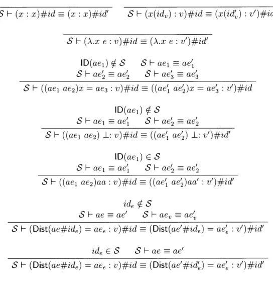
Figure 2-7 presents the definition of =. Note that operating with entangled subprob-lems forces the inference tactic IT to take the full program trace t as a parameter even though it must modify at most only the subproblem.

S - (x(id,) : v)#id = (x(id') : v')#id'

S F- (A.x e : v)#id - (A.x e : v')#id'

ID(ae1) ( S

S - ae' ae'

S F- aei - ae' S F- ae' ae'

S - ((aei ae2)x = ae3 : v)#id - ((ae' ae')x = ae' : v')#id

ID(ae1) S

S F- aei1 ae' S Fae' ae'

S - ((aei ae2) I: v)#id = ((ae' ae') I: v')#id'

ID(ael) E S

SF- aei =ae' S F-ae' - ae'

S - ((aeI ae2)aa : v)#id = ((ae' ae')aa' : v')#id'

ide S

S - ae = ae' S - ae, = ae'

S F (Dist(ae#ide) = ae, : v)#id - (Dist(ae'#ide) = ae' v')#id' ide E S S F ae = ae'

S - (Dist(ae#ide) = aee : v)#id - (Dist(ae'#id') = ae' v')#id'

(a) Equivalence Check over augmented expressions, =- P(ID) x P(ID) x aE x aE

S - ae = ae'

S - 0 - 0

S F- t t'

S F assume x = ae; t = assume x = ae'; t'

S F- ae = ae' S F- t t'

S F- observe(Dist(ae#id) = ev); t - observe(Dist(ae'#id) = e,); t'

(b) Equivalence check over traces, C= P(ID) x P(ID) x T x T Figure 2-7: Equivalence Check for correct Inference S -(x : x)#i~d =- (x : x)#id'

Chapter 3

Independent Subproblem Inference

The basic idea of independent subproblem inference is to extract an independent sub-trace t, from the original sub-trace t given a subproblem S, perform inference over the extracted subtrace t, to obtain a new trace t', then stitch t' back into t. Here, consis-tent with standard inference techniques for probabilistic programs [24j, ts and t's are valid traces of the same program Ps (the subprogram for the subtraces t, and t'). The key challenge is converting the entangled subproblem (which is typically incomplete and therefore not a valid trace of any program) into a valid trace by transforming the subproblem to include external dependences and correctly scope both internal and external dependences in the extracted trace without given the inference algorithm ac-cess to any external stochastic choices (including latent choices nested inside certain lambda expressions which would otherwise override choices outside the subproblem) which it must not change.

Extract Trace: I define the extraction procedure ts = ExtractTrace(t, S) using the

transition relation -+ex P(ID) x P(ID) x T -+ T (Figure 3-1).

The extraction procedure removes Dist(ae#id) = ae, augmented expressions which are not within the subproblem and converts them into observe statements. This transformation constrains the value of these stochastic choices to the values present in the original trace. It leaves the stochastic choices in the subproblem in place and therefore accessible to the inference algorithm.

S F (x(id') v)#id -ex (x(id') : v)#id, 0

S I- (x: x)#id =ex (x : x)#id, 0

S F (A.x e v)#id =ex (A.x e : v)#id, 0

ID(aej) E S S F- aei sex ae'1, ts S - ae2 ex ae', t'

S - ((aei ae2)aa: v)#id ==>ex ((ae' ae')aa: v)#id, t,; t'

ID(aej) S S F- aei =e2x ae', ts S F- ae2 >ex ae', t'

S F- ((aei ae2) I: v)#id, tP >ex ((ae' ae') I: v)#id, ts; t'

ID(aej) S

S - ae2 *ex ae', t'

S F- ae1 *ex ae'i, t

S F- ae3 =e> aex',t''

x <- Fresh variable name

t'"= ts; assume x = ae'; t'; assume y = ae'2 ; t''

S F ((aei ae2)y = ae3 : v)

#id,

tP ex ae' , t'"

id' ( S S F ae e,ae',t, aev =tr ev S F- aev ='>ex aet, t'

S - (Dist(ae#id') = ae: v)#id we, ae', t,; observe(Dist(ae'#id') = ev); t'

id' E S S F ae =ex ae', ts

S F- (Dist(ae#id') = aev : v)#id 4,e (Dist(ae'#id') = aev : v)#id, ts

(a) Extracting subtrace from an Augmented Expression, e>xg P(ID) x P(ID) aE x T

id = ID(ae)

S F ae >ex ae',ts S F- t ex t'

S F- 0 weX 0 S F- assume x = ae; t wex t8; assume x = ae'; t'

S F- ae wex ae' t S F- t -=ex t'

S F- observe(Dist(ae#id) = e,); t -=ex t,; observe(Dist(ae'#id) = e,); t'

(b) Extracting subtrace from a given trace, wexg P(ID) x P(ID) x T -+ T

Figure 3-1: Extraction Relation

S F- (x : v)#id,(x : v')#id', tp _{=-t (x : v')#id', t,}

S - (x(id,) : v)#id, (x(id') v')#id', t =p t (x(id') : v')#id', tp

S F- (A.x e : v)#id', (A.x e v')#id, tp est (A.x e : v')#id, t,

ID(ae') E S S F- ae', ae2, t,

ast

ae', t' S - ae', aei, t' =,t ae", t''

S - ((ae' ae'2)aa' : v')#id', ((aei ae2)aa : v)#id, t -ist ((ae" ae')aa : v)#id, t"

ID(S'F', ae' V S ae', a 3, t =t

S & ae' ae2, t' ==>t ae'2' t"; assume x = aei

ae', t'; assume y = ae2

S - ae', aei, t" >st ae", t'"

S F- ((ae' ae')y = ae' : v') #id, aC3, t, e ((ae" ae')y = aez : V(ae'))1#idt

ID(ae') S S -ae' ae2, t, ,t ae'2 t' S F- ae', ael, t' .st ae"l, t" S F- ((ae' ae') I: v')#id', ((ae1 ae2) I: v)#id, t, eSt ((ae' ae') I: v)#id, t"

id' cS S - ae', ae,t, =>Mt ae", t'

S - (Dist(ae'#id') = ae' : v')#id', (Dist(ae#idv) = aev : v)#id, t, st (Dist(ae#idv) = aev : v)#id, t'

id', V S S F- ae', ae, t ==>st ae', t'; observe( Dist(ae#id',) = ev)

S F- ae', ae, t' *st ae", t"

S F (Dist(ae'#idv) = ae' : v')#id', aen, - st (Dist(ae#idv) = ae' : V(ae'))#id, t' (a) Stitching augmented expressions, =:stg P(ID) x P(ID) x aE x aE x T -+ aE x T

S F- ae, ae' t, ==st ae", t' S - t, t' e'st t'

S F- 0, 0 est 0 S - t; assume x = ae, tp; assume x = ae' -i>st assume x = ae"; tS

S F- ae, ae', t, =' st ae",t' S - t,t, -=st t'

S F- t; observe(Dist(ae#id) = ev), tp; observe(Dist(ae'#id') = ev) ->st observe(Dist(ae"#id) = ev); t'

(b) Stitching trace and subtrace, wtC P(ID) x P(ID) x T x T -+ T

subproblem, its value can change and hence existential edges place the augmented expressions in ae3 within the subproblem. When ae1 is not within the subproblem, then some stochastic choices may or not be within the subproblem. If I keep the augmented expression as is, the inference algorithm may unroll ae3 and execute it again, changing some stochastic choices in ae3 but not in the subproblem. If I modify

ae, the constraint of ae3 being a valid lambda application breaks. I solve this problem by introducing assume statements and correctly scoping the resulting dependences. Stitch Trace: Given a trace t, a valid subproblem S over the trace and a subtrace

ts, the stitching procedure stitches back the trace ts into t to get a new trace t'.

I define the stitching procedure t' = StitchTrace(t, to, S) using a transition relation

>sSt P(ID) x P(ID) x T x T - T (Figure 3-2). Stitching is the dual of extraction.

It uses the original trace to figure out the structure of the resultant trace and stitches back the expressions to get a new trace t'.

Independent Inference: I define independent subproblem inference using the infer procedure. infer takes as input a subproblem selection strategy SS, a trace t and an inference tactic IT. This differs from tangled inference in that inference tactic IT takes only the extracted subtrace as input and not the entire program trace. This approach enables the use of standard inference algorithms which are designed to operate on complete traces (and not entangled subproblems).

The new inference procedure works as described below:

SS(t) = S ts = ExtractTrace(t, S) t' = IT(ts)

t' E Traces(Program(ts)) t' = StitchTrace(t, t', S)

infer(SS, IT), t = t' (3.1)

Soundness and Completeness: Given a trace t, a valid subproblem S, an infered trace t' and ts = ExtractTrace(t, S), I prove that my subprogam inference method of extraction and stitching is sound and complete. Soundness in this context means that for all possible mutated subtrace t' E Traces(Program(ts)), the stitched trace

t'

c Traces(Program(t))

S - t ' t t' rn r) t, ts t,ts t' E Traces(Program(t,))

Figure 3-3: Entangled vs Independent Subproblem Inference

that for all possible infered traces t', there exists a mutated subtrace t' such that

t' E Traces(Program(ts)) and t' = StitchTrace(t, t', S).

I summarize the comparison between the entangled subproblem inference and independent subproblem inference approaches in Figure 3-3

I present the theorems, lemmas and their respective proofs to prove the soundness and completeness of my interface below.

3.1

Soundness

Observation 1. Note that whenever a rule in wex introduces an assume statement

in the subtrace, it creates a new variable name. Therefore variable names in the new subtrace do not conflict with any variable names previously introduced in another part of the trace. This fact will be used at various points within this paper.

Observation 2. Note that whenever S I- ae wex aes, t, V(ae) = V(ae,) and

when-ever S I- ae, aes, ts =st ae', V(ae') = V(ae,).

To prove soundness of our interface we start by proving that for a given trace t and a valid subproblem S on trace t, if for any subtrace ts the stitching process succeeds, the output trace t' differs from trace t only in parts which are within the subproblem

(i.e. S n

t tc t').

Formally, for any trace t and subproblem S,

= StitchTrace(t, t,, S) - S t- t'

Using the definition of StitchTrace, the above lemma can be rewritten as

S _ t, _ = St t' =-> S - t =_ t'

One will note that the stucture of ts does not play a significant role in proving the above condition.

To prove the above statement we require a similar condition over augmented ex-pressions embedded within traces. The lemma over augmented exex-pressions is given below:

Lemma 1. For all augmented expressions ae, ae',

S H ae, _, _ ts ae', -=> S F- ae = ae'

Proof. Proof using induction.

Base Case:

Case 1: ae = (x : x)#id,

By assumption

S I- ae, -, - =st ae', _

By definition of >st

S

F-

(x : x)#id' _, _ _{est (x : x)#id', _}

By definition of =

S H (x: x)#id = (x : x)#id' Therefore

S H ae = ae'

Therefore when ae = (x: x)#id,

S H ae, _, _ est ae', _ = S H ae = ae'

Case 2: ac = (x(id,) v)#id

By assumption

S & ae, _,_ st ae',

By definition of e4

st

S

H

(x(id,) : v)#id, _, _ >st (x(id') : v')# -d'

Then ae' = (x(id',) : v')#id'. By definition of

-S H (x(idv) : v)#id = (x(id',) : v')#id'

Therefore

S H ae - ae'

Therefore when ae = (x(id,) : v)#id,

S k ae, _ _ ae

Case 3: ae = (A.x e : v)#id

By assumption

== S H ae = ae'

By definition of >st

S

H

(A.x e : v)#id, _ _ =st (A.x e : v')#id',

Then ae' = (A.x e : v')#id'. By definition of

S H (A.x e : v)#id (A.x e : v')#id'

Therefore

S H ae ae'

Therefore when ae = (A.x e : v)#id,

==> S H ae = ae'

Induction Cases:

Case 1: ae = ((aei ae2) I: v)#id and ID(ael) ( S

By assumption

S - ae, _, _ st ae'1

By definition of est

S H ((aei ae₂) I: v)#id, __ _ =st ((ae1 ae) I: v')#id', _{_}

Then ae' = ((aei ae2) I: v')#id', S H aei, _, _

ae2,

_-By induction hypothesis

S & ael, _,_ st ae',_

Because S H ael, _, _ *st ae',

-S H ae1 - ae'

ae', _, and S H ae2,

-==- S H ae1 - ae'

By induction hypothesis

S H- ae2, , _ st ae', _ S H ae2 ae'2

Because S H ae2, _, _ -st ae'2,

S H ae2 = ae'2

Because S H aei ae' and S H ae2 ae', by definition of

S H ((aei ae2) I: v)#id ((ae' ae') I: v')#id'

Therefore

S H ae ac'

Therefore when ae = ((aei ae2) I: v)#id,

S & ae, _, _ -st ae' => S H ae ate

Case 2: ae = ((ae ae2)aa : v)#id and ID(ae1) E S

By assumption

S E ae, _, >st ac'

By definition of ast

S

H

((ae ae2)aa : v)#id, _, ->st ((ae' ae')aa' v')#id', _

Then ae' = ((aei ae2)aa' : v')#id', S H ael, _, _ -st ae', _, and S H ae2, _, _ ae2, .

By induction hypothesis

S

H

aei, _, _ =>st ae', _ ==> S H aei = ae'

Because S F ael, _, _ zst ae', -S F ae1 = ae' By induction hypothesis S ae2, _, _ -st ae'2, _ --

>

S ae2 = ae' Because S F ae2, _, - st ae', -S F ae2 - ae'

Because S F ae1 = ae' and S F ae2 - ae', by definition of

S F ((aei ae2)aa : v)#id = ((ae' ae')aa': v')#id'

Therefore

S F ae = ae' Therefore when ae = ((aei ae2)aa: v)#id,

S & ae, -, - ->st ae', _ =- S F ae = ae'

Case 3: ae = ((aei ae2)X = ae3 : v)#id and ID(aei) S

By assumption

S E ae,, _>st ae' _

By definition of -t>,

S - ((aei ae2)X = ae3 : v)#id _, _ -st ((ae' ae2)y = ae' :

Then ae' = ((ae1 ae2)y = ae'

ae2, _, _ ->st ae',

By induction hypothesis

S H aei, _, _ st ae', _

Because S H aei, _, - est ae',

-S F- aei = ae' By induction hypothesis S H ae2, -, _ est ae2, _ Because S H ae2, _, _ =st ae'2, S H ae2 = ae'2 By induction hypothesis

S H ae₃, _ - =st ae',_ -- > S & ae₃ ae'

Because S H aC3, , _ e't ae',

S H ae3 = ae3

Because S aei = ae', S & ae2 ae' and S & ae3 ae', by definition of

S H ((aei ae2)x = ae3 : v)#id - ((ae' ae')y = ae' : v')#id'

Therefore

S H ae = ae'

= S H ae1 = ae'

Therefore when ae = ((aei ae2)x = ae3 : v)#id,

S E ae, _, _ =:s ae', _ ==- S H- ae = ae'

Case 4: ae = (Dist(aei#ide) = ae2) : v)#id and ide S.

By assumption

S & ae,, = st ae',

By definition of -st

S H (Dist(aei#ide) = ae2) : v)#id, _->st (Dist(ae'#ide) = ae') : v')#id',

Then ae' = (Dist(ae'#ide) = ae') : v')#id', S H aei, _, _

ae2, _, _ -st ae',

_-By induction hypothesis

S & ael, _, _ ->st ae',

-Because S H aei, _, - =>st ae',

--->st ae', _, and S H

-- > S H aei = ae'

S H ae1 = ae'

By induction hypothesis

S H ae₂, _ _ stae₂, --- S H ae2 - ae'

Because S H ae2, _, - ast ae',

-S H ae₂ - ae'

Because S H aei 1 ae' and S H ae2 - ae', by definition of

Therefore

S F- ae ae'

Therefore when ae = (Dist(aei#ide) = ae2) v)#id and ide S,

S F ae, _, _ *st ae _ ==- S F- ae = ae'

Case 5: ae = (Dist(aei#ide) = ae2) : v)#id and ide E S.

By assumption

S F ae, __ _ae

By definition of >st

S F- (Dist(aei#ide) = ae2) : v)#id,-, - Mst (Dist(ae'#ide) ae') v')#id',

Then ae' = (Dist(ae'#id,) = ae') : v')#id' and S I- aei, _, _ -st ae',

By induction hypothesis

S F- ael, _, _ >st ae', _ = S F- aei = ae' Because S I- aei, _, _>,t ae', _

S F- aei ae'

Because S F ae = ae', by definition of

S F (Dist(aei#ide) = ae2) : v)#id (Dist(ae'Z#ide) = ae') : v')#id'

Therefore

Therefore when ae = (Dist(aei#ide) = ae2) : v)#id and ide E S,

S F- ae, -, - ->st ae', - ==- S F- ae - ae'

Because all cases are covered, using induction, the following statement is true for all augmented expressions ae, ae' and subproblems S.

S F ae, _, _ -t ae', == S ae = ae'

Next we use Lemma 1 to prove the lemma below::

Lemma 2. Given traces t and t' and a subproblem S, S - t, _ ->,t t' - S - t =- t'

Proof. Proof by Induction

Base Case: t 0 By assumption S -t _ -- st t' By definition of ->st S F 0, _ ->st 0 Then t' = 0. By definition of SF-0 0 Therefore S F- t t' Therefore when t = 0 S

-t

_ -> = tt' == S F- t = t'

Induction Case:

Case 1: t = t,; assume x = ae

By assumption

S

F-

t, _ z>t'

By definition of zst

S F- t,; assume x = ae, _ = st t's; assume x = ae'

Then t' = t'; assume x = ae', S F ae, _ _ >st ae' _, and S F-ta, _ st t* By induction hypothesis

S -ts, _ et t', -o S

-

t,

=

t'

Because S - ts, _ stt s

S F- ts = t'

From Lemma 1

S F ae, _, _ >st ae' I =w S F- ae ae'

Because S F- ae, -, - >st ae', _

S F- ae = ae'

Because S F t' to, and S F- ae = ae', by definition of

S F- ts; assume x = ae t's; assume x = ae'

Therefore

S F- t t'

Therefore when t = ts; assume x = ae

Case 2: t = t,; observe(Dist(ae) = e,)

By assumption

S -t _ -st t,

By definition of -st

S H t ; observe(Dist(ae) = e,), _-st t'; observe(Dist(ae') = e,)

Then t' = t'; observe(Dist(ae') = e,), S H ae, -_>st ae', _, and S H ts, _ ->st t'. By induction hypothesis

Because S F t, _ ->t ts

S H to t'

From Lemma 1

S & ae, _, _ ->st ae', _ => S H ae = ae'

Because S & ae, _, - ->st ae', _

S H ae - ae'

Because S H t' ts and S H ae = ae', by definition of

S H t,; observe(Dist(ae) = e,) t'; observe(Dist(ae') = eV)

Therefore

S H t '

Therefore when t = ts; observe(Dist(ae') = ev)

S t, _ -t t' ->4 S

0 t -t'

Because all cases have been covered, using induction, for all traces t, t', subproblems S and subtrace to,

S _ tits = -t t' -e S - t -= t'

Corollary 1. Given a valid trace t, a valid subproblem S, a valid subtrace ts, for all

traces t' :

t' = StitchTrace(t, t,, S) ==- S - t - t'

Therefore, given a trace t and a valid subproblem S on t, if the stitching process succeeds, then the output trace t' will only differ from trace t with parts which are within the subproblem S.

Next, we prove that given a valid trace t, a valid subproblem S on trace t, and a subtrace ts = ExtractTrace(t, S), for any subtrace t' E Traces(Program(t,)), the stitched trace t' = StitchTrace(t, t', S) is a valid trace from the program of trace t (i.e.

t'

c

Traces(Program(t))).

Formally, given a valid trace t, a valid subproblem S on t, and a subtrace ts =

ExtractTrace(t, _S),

V t'

c Traces(Program(t,)).

t' = StitchTrace(t, t', S) A t'

E

Traces(Program(t))

To prove the above statement, we require a few lemmas first which prove a similar condition for augmented expressions and traces under non-empty environment Lemma 3. Given environements O-,, Uid,oj and o dv such that dim = dom

ai-dom or' = ai-dom o0-s an augmented expression ae within a trace t, and a valid subproblem

S over trace t

3 e, ps.c-O, ci He =_ - , _, ae A S H- ae >, aes, ts

Ats; assume z = aes =' r ps A o-, /id H Ps =>s ts; assume z = ae'I

Proof. Proof by induction Base Case: Case 1: ae = (x : x)#id By assumption Uv, id e = s _, _ , ae By definition of *s

aO'v, Oid F- X = _, -, (x : x)#id

Then e = x and x dom o-. By assumption

S F- ae ='>e, aes, ts

By definition of wex

S F- (x : x)#id =ex (x : x)#id, 0 Then aes = (x : x)#id and ts = 0.

By assumption

t,; assume z = ae, 4 _{, ps}

By definition of 4r

assume z = (x : x)#id r, assume z = x

Then ps = assume z = x. By assumption

oU, ,Oid FPS =psS t's; _{assume z} = aes By definition of >s, dom o- = dom

a-Of, a/ F- assume z = x => assume z = (x : )#id'

Consider ae' =

(x

: x)#id'.

By definition of =st

S H (x : x)#id, (x : x)#id', 0 zst (x : x)#id'

Therefore

S H ae, ae', t' >st ae'

By definition of => and x c dom a'

ofI orI u id x x= x _,, (x : xiz I)#zd'

Therefore

OU ,Jodl e =s _ , _ , ae'

Therefore when ae =

(x

: x)#id

3 e, ps.-Ui d o- e 8, _, ae A S & ae we, aes, ts

At,; assume z = ae, >, p, A o, oiYd H Ps =S ts; assume z _{= aes}

- ae'.S ae, ae', t' =st ae' _ A o, or H e = _, _, ae'

Case 2: ae = (x(idv) : v)#id

By assumption

-,

cd

H

e = _, _, ae

By definition of >s

O'v Uid H- Xv = -i -, (cv(idv) : v)#i'd

Then e = x, v = u(x), and idv = gd(X). By assumption

By definition of ex

S H (x(idv) : v)#id #,ex (x(idv) : v)#id, 0

Then ae, = (x(idv) : v)#id and t, = 0.

By assumption

t,; assume z = ae, ==>, ps

By definition of 4r

assume z = (x(idv) : v)#id =i, assume z = x

Then p, = assume z = x.

By assumption

O-', od F Ps >s t',; assume z = ae'

By definition of , dom o' = dom

a-a I, or/ F- assume z = x =a assume z = (x(id') v')#id'

Then t' 0, ae' = (x(id',) : v')#id', v' = o'(x), and id', = c d x. Consider ae' = (x(id',) : v')#id'.

By definition of est

S - (x(idv) : v)#id, (x(id',) : v')#id', 0 >st (x(id',) : v')#id'

Therefore

S - ae, ae', t' =>st ae'

By definition of =8 ,v' = o'(x), and id', = Od(

Therefore

-', a e as _, _, ae'

Therefore when ae = (x(id) : v)#id

E e, s 0v, o-d F- e =- _, _, ae A S I- ae =>,x aes, ts

Ats; assume z = aes =, ps A ou/, 1 H- pS =s>S t's; assume z = ae' -1 ae'.S -ae, ae', t' =st ae' _ A o-', i F- e => ,,ae'

Case 3: ae = (A.x e' : v)#id

By assumption

ov, id H e =s _, _, ae

By definition of as

U-v, Uij - A.x e' =>s , , (A.x e' : v)#id

Then e = A.x e'.

By assumption

S F- ae >ex aes, ts By definition of zex

S F- (A.x e' : v)#id =>ex (A.x e' : v)#id, 0

Then aes = (A.x e' : v)#id and t, = 0.

By assumption

t,; assume z = aes >r ps

By definition of >r

Then p, = assume z = A.x e'.

By assumption

i, H

F Ps as ts; assume z = ae'

By definition of >s, dom a-' = dom o-,

o-' I-a - assume z = A.x e' =a assume z = (A.x e' v')#id'

Then t' = 0 and ae' = (A.x e' : v')#id'.

Consider ae' = (A.x e' : v')#id'. By definition of #=st

S H (A.x e': v)#id, (A.x e': v')#id', 0 *st (A.x e': v')#id'

Therefore

S ae, ae', t' zst ae'

By definition of =s and o-', or' H A.x e' a _, _, (A.x e' : v')#id'

or',, or a F A.x e' =#s __,(A.x e' : v')#Zd'

Therefore

ao 1, / a F e ==s __,ae', id

Therefore when ae = (A.x e' : v)#id

E e, ps.av, aide s -, -, ae A S H ae ex aes, ts

Ats; assume z = ae, = , ps A av d H Ps =s t'; assume z = aeS

-= ae'.S ae ae', t'8 5 t ae', _ Aol, a - e S, ,ae

Induction Cases:

By assumption

0_{v , aid F e}

~>s _ _, ae

By definition of

-O-v, ad F- Dist(ei) = -, _, (Dist(aei#ide) = aev : v)#id

Then e = Dist(ei), o-v, ad F- e1 = _, , ae₁.

By assumption

S - ae ->ex aes, t₈

By definition of --ex

S F- (Dist(aei#ide) = aev : v)#id ->ex (Dist(ael#ide) =

Then aes = (Dist(aei#ide) = aev : v)#id, ts = t', and S aei e, ae, tI.

By assumption

t,; assume z = aes ->, ps

By definition of =>,

assume z = (Dist(ae'#ide)= _{aev : v)#id >, assume z = Dist(el)}

Then ps = pl; assume z = Dist(e') and ael ->, e'.

By assumption

P , -=4>S t's; assume z = ae'

vI aidr _S

By definition of =>,

o-', - F p; assume z = Dist(ei) - ; assume z = (Dist(ae2#id') Sae : v')#id'

Then t' = ts, ae' = (Dist(ae #ide) = ae' : v')#id', and a', F- ps; assume z =

ei - t ; assume z = ae2.