Computation of the one-dimensional unwrapped phase

Computation of the One-Dimensional

Unwrapped Phase

by

Zahi Nadim Karam

Submitted to the Department of Electrical Engineering and Computer

Science

in partial fulfillment of the requirements for the degree of

Master of Science in Electrical Engineering

at the

MASSACHUSETTS INSTITUTE OF TECHNOLOGY

) Massachusetts

January 2006

Institute of Technology 2006.

All rights reserved.

Author

...

Department of Electrical Engineering and Computer Science

January 24, 2006

Certified

by

...

_{Alan V. Oppenheim}

.a.

.

.

i

Ford rofessor of Engineering

Department of

Electrical Engineering and Computer Science

)

Thesis Supervisor

.. , / A

~~-,,

Accepted by ...

'.

--ArthU4 C. Smith

Chairman, Department Committee on Graduate Students

Department of Electrical Engineering and Computer Science

ARCHIVES MASSACHUSE'n OF TECHN

JUL 10

Computation of the One-Dimensional

Unwrapped Phase

by

Zahi Nadim Karam

Submitted to the Department of Electrical Engineering and Computer Science

on January 24, 2006, in partial fulfillment of the requirements for the degree of

Master of Science in Electrical Engineering

Abstract

In this thesis, the computation of the unwrapped phase of the discrete-time Fourier

transform (DTFT) of a one-dimensional finite-length signal is explored. The phase of

the DTFT is not unique, and may contain integer multiple of 27r discontinuities. The

unwrapped phase is the instance of the phase function chosen to ensure continuity.

This thesis presents existing algorithms for computing the unwrapped phase,

dis-cussing their weaknesses and strengths. Then two composite algorithms are proposed that use the existing ones, combining their strengths while avoiding their weaknesses. The core of the proposed methods is based on recent advances in polynomial factoring.

The proposed methods are implemented and compared to the existing ones.

Thesis Supervisor: Alan V. Oppenheim

Title: Ford Professor of Engineering

Acknowledgments

I would like to thank my family for all their love, commitment and support. Pop,

you've always been my role model. Mom, your tenderness and unconditional love

al-ways made me feel warm and safe. Amme, for your wisdom, moral guidance and

youthfulness. Hanan, your compassion and selflessness have always inspired me.

Samer, for your determination, sense of adventure and passion for life. Amme Najwa

and Amme Salwa for always being there and more. Teta and Jiddo, for your love and

confidence.

To my advisor Al Oppenheim. You've been there from day one, making sure that

my transition into MIT was smooth, comfortable and successful. Thank you for your

wisdom, care and guidance. Your passion for teaching, your out of the box thinking

and your sense of adventure have inspired me.

Alaa Kharbouch (3alaa2). We've watched each other's back since freshman year.

We are complete opposites, and yet best of friends. Thank you for sharing the pain

and the experience.

Amer Abufadel, you're like a big brother to me. You got me started, and have always watched out for me.

I would like to thank the DSPG: Joonsung for tolerating me and for being a great

office mate. Petros for always having the answer. Sourav for the playful atmosphere

and the long discussions. Tom for your musical ear. Maya for your help. Eric for

your willingness to always help. Ross and Matt, Alecia, Charlie, Melanie, Dennis,

Archana, Joe and Andrew, for making the office a pleasant place to hang out.

Prof. Vivek Goyal, thank you for a wonderful and stimulating experience working on the class with you. Prof. George Verghese thank you for looking out for me.

To all my friends, thank you for adding flavors and purpose to my life. Alieh,

thanks for your love, care and advice. The Atrashes, thanks for being there for me.

Victor, we've shared a lot of experiences together, thank you for being a great friend.

Akram, thank you for the encouragement and support. Yousef, Woody, Pierre, Loucy,

and George thanks for all the crazy times we've had, my breaks in Lebanon would not

have been the same without you. Wafaa2, Cathy, Pranav, Demba, Tamer, Viktorija,

Lololna, Chrisann, Sandra, Lara, Zaid, Lolita and Mauri thanks for your friendship

and for making my life in the US not just about study and work.

Contents

1 Introduction and Background

15

1.1 Problem Statement ...

16

1.2 Instances of the Phase and the Derivative of the Unwrapped Phase .

17

1.2.2 Derivative of the Unwrapped Phase . . . 19

1.2.3 Unwrapped Phase . . . ... 19

1.3 Example Phase Functions ...

21

2 Existing Algorithms to Compute the Unwrapped Phase

23

2.1 Phase Unwrapping by Detecting Discontinuities .

...

23

2.2 Phase Unwrapping Using Adaptive Numerical Integration ...

26

2.3 Computation of the Unwrapped Phase Using Polynomial Factoring .

28

2.4 Phase Unwrapping from the Time Series

.

...

29

2.5 Iterative Method to Compute the Unwrapped Phase ...

30

2.6 Phase Unwrapping by Isolating Sharp Zeros . ... 31

2.7 Summary ... 32

3 Method for Factoring High Degree Polynomials

33

3.1 Outline of the Algorithm ...

33

3.2 Deflation Failure ... 34

3.3 Discussion ... 35

4.1 Motivation ...

4.2 Overview ...

4.3 Polynomial Factoring and Deflation ...

4.3.1 Steps to Find Zeros Close to the Unit

4.3.2 Search Grid ...

4.3.3 Deflation ...

4.4 Modified DD and ANI Algorithms ... 4.4.1 Modified DD Algorithm ...

4.4.2 Modified ANI Algorithm ...

4.5 Robustness To Errors In Factored Zeros . .

4.6 Summary ...

5 Algorithm Evaluation

5.1 Algorithm Evaluation Using Synthetic Signals ...

5.1.1 Synthetic Signal with Zeros Close to the Unit Circle ...

5.1.2 Synthetic Signal with Zeros Far from the Unit Circle ...

5.1.3 Synthetic Signal with Zeros Close to and Far from the Unit Circle

5.1.4 Large Number of Synthetic Signals with Randomly Chosen Zeros 5.1.5 Discussion ...

5.2 Algorithm Evaluation Using Speech Data ...

5.2.1 Speech Data ...

5.2.2 Filtered Speech Data ...

5.3 Algorithm Evaluation Using EEG Data ...

5.3.1 EEG Data ...

5.3.2 Filtered EEG Data ...

5.4 Summary ...

A Zeros of Random Polynomials

A.1 Zeros of I.I.D. Random Polynomials ...

A.2 Zeros of Bounded Coefficient Random Polynomials ...

37 38 39 39 40 42 43 43 44 44 46

47

B Cepstrum Bibliography

B.2 Computation ...

B.3 Speech/Audio ...

B.5 2D/Image ...

B.8 Applications ...

B.9 Other ...

67

... .

67

... .

69

... .

70

... .

88

... .

88

... .

90

... .

92

... .

92

... .

97

...

...

...

...

...

...

...

...

List of Figures

1-1 Example Wrapped Phase Function ...

18

1-2 Example unwrapped phase ...

20

1-3 Unwrapped phase and phase derivative ...

21

1-4 Unwrapped phase, principal value of the phase, and phase derivative.

22

2-1 Unwrapped phase using detection of discontinuities ...

25

2-2 Unwrapped phase using adaptive numerical integration ...

28

2-3 Sample Search Grid ... ... 29

3-1 Z-plane plots demonstrating deflation failure ... 35

4-1 Block diagram of proposed algorithms ... 39

4-2 Block diagram for the polynomial factoring part of the algorithm

.

40

5-1 Results for the synthetic signal with zeros close to the unit circle.

.

49

5-3 Results for the synthetic signal with zeros close to and far from the

5-4 Speech segment of the utterance "Unwrapped Phase" .

...

54

5-5 Results for speech data. ... 55

5-6 Results for filtered speech data. ... .. 56

5-7 EEG data while performing a multiplication task .

...

57

5-8 Results for EEG data. ...

58

A-1 Observed clustering near the unit circle of zeros of polynomials with i.i.d. uniformly distributed random coefficients. ... 63 A-2 Observed clustering near the unit circle of zeros of the z-transform of

List of Tables

5.1 Results for the synthetic signal with zeros close to the unit circle. ..

50

5.2 Results for the synthetic signal with zeros far from the unit circle. .. 50

5.3 Results for the synthetic signal with zeros close to and far from the unit circle ... 51

5.4 Results from 2000 synthetic signals ... 53

5.5 Results for speech data. ... 54

5.6 Results for filtered speech data. ... 56

5.7 Results for EEG data. ...

57

Chapter 1

Introduction and Background

Homomorphic signal processing with the complex cepstrum [1] has been applied, with considerable success, to many areas of digital signal processing [3], most notably speech, seismric and EEG data processing. The computation of the complex

cep-strum requires obtaining the unwrapped phase, which is the continuous and periodic

instance of the phase of the discrete-time Fourier transform (DTFT) of the input

signal. Refer to Appendix B for a bibliography we have compiled on the complex

cepstrum.

The phase of the DTFT, however, is in general ambiguous since at any frequency 27rk (k is an. integer) can be added without affecting the result of the complex expo-nentiation [1]. This ambiguity, therefore, allows the phase of the DTFT to contain

discontinuities in the form of 27rk jumps. The unwrapped phase is the instance of

the phase function where the additive integer multiples of 2r at each frequency are chosen to ensure that it is continuous; therefore, it is suitable for the computation of

the complex cepstrum.

Reliably computing samples of the unwrapped phase of a given mixed-phase signal is an open problem: existing algorithms are not reliable and in many cases fail. The

difficulty of computing the unwrapped phase carries over directly to the computation

of the complex cepstrum. This thesis presents two composite algorithms that use

the existing ones. The reliability and accuracy of the proposed algorithms have been

demonstrated through numerous experiments, the goal being to render homomorphic

signal processing using the complex cepstrum more computationally reliable.

1.1 Problem Statement

The complex cepstrum is a sequence i[n] that is related to a discrete-time signal x[n] by the following invertible transformation,

00

X(z) = E

x[n]z-n=-oo

X(z) = log(X(z))

[n]

=

2

.

j

f (z)zn-'dz.

For [n] to be a stable sequence we require that the region of convergence of X(z)

contain the unit circle, which leads to the equivalent relationships

X(e")

=

log[X(ej)lej

_e

_(1.1)

= log

IX(ejw)l

1 (r

x[n] = X(ew)ewndw. (1.3)

The angle 4X(eiw) in Equation (1.2) is only unique to an additive multiple of

27r at each frequency w; therefore, the imaginary part of X(ejw) is ambiguous. To remove this ambiguity and for X (ej ) to exist we require that <X(ejw) be a continuous

function of w. The unwrapped phase arg IX(eJw)l is defined as the unique instance of

qX(eu'),

arg IX(ejw)l = 4X(ei

) + 27rk(w)

kEZ,

(1.4)

where the additive multiple of 2ir at each frequency is chosen to satisfy the continuity

condition.

For k(ejw) to be a valid DTFT of the complex cepstrum i[n] it must be periodic

the input signal is real, the complex cepstrum is also real and X(edw) is a conjugate

symmetric function. This implies that when the input signal is real, the unwrapped

phase function is odd symmetric. Refer to [1] for more details on the complex

cep-strum and its properties.

Reliable computation of the unwrapped phase is an open problem to which

exist-ing solutions cannot guarantee accuracy for any given input sequence. The difficulty

of the problem becomes apparent in the next chapter where existing algorithms are

presented. This thesis focuses on computing the unwrapped phase of the DTFT of

finite-length discrete-time signals.

1.2 Instances of the Phase and the Derivative of

the Unwrapped Phase

In this section we present two instances of the phase function: the unwrapped phase

and the principal value of the phase. We also present the derivative of the unwrapped

phase.

A finite-length discrete-time signal x[n] has a z-transform of the form

Mi Mo

X(z) = Azr

H7(1

J(1

k=l k=l

Mi corresponds to the number of zeros inside the unit circle, and Mo the number

outside. The term

is a time shift that contributes a linear phase term with slope r.

When the signal is causal r = -M,. A is real when x[n] is real. The phase of X(ejw)

is, therefore, equal to

~Mi

:X(e

_{) = A + e}

_{wr + E}

₍₁

_-ake

_i)

₊

_E

₍₁

_-

_bkel).

_(1.6)

1.2.1 Principal Value of the Phase

Section 1.1 presented the unwrapped phase arg X(ejW)I as a unique instance of the

phase function. Another unique instance is the principal value ARGX (ew) for which

the 27r ambiguity is removed by restricting the value of ARGIX(ej)l at any w to the

range [-r, 7r[.

The principal value can be calculated using the arctangent routine

ARG[X(eJ")] = arctan( X(e)

)

(1.7)

XR(e)

(1.7)

where the subscripts

and I denote the real and imaginary parts. This calculation

clearly forces

-or < ARG[X(edw)] < r,

(1.8)

and thus values of the phase outside this range will be "wrapped" so that they fall

within it; for this reason the principal value is sometimes referred to as the "wrapped

phase". The wrapping causes the principal value to have discontinuities in the form

of jumps of 27r as seen in Figure 1-1. It is also important to note that

~~Mi ~Mo

ARGIX(eJw)I = mod{ARGIAI+ARGIdrI+Z-+ ARGI(1-ake-ij)+E ARGI(1-bkew)lI}2..

k=l k=l

(1.9)

Prlnolpol Vluo of the Phm6e 4 3 2 -2 -a3 -4 0 1 2 3 4 5 6 7

1.2.2 Derivative of the Unwrapped Phase

The phase derivative arg' IX(eJ)] is the derivative of the unwrapped phase with

respect to w. Exact values of the derivative may be computed using

x'(ej-

arg'

IX(ew)

=

{ X(e) I

(1.10)

XR(ejW)X(ejw)-XI(ejw)XR(ejw)

where £{W} is the imaginary part of W, the superscript ' denotes differentiation

with respect to w, and X'(ejw) can be obtained by:

00

X'(e

_{) =}

_(-jnx[n])e

_(1.12)

n=-oo

The derivative is a linear operator and therefore

~~Mi ~Mo

arg' IX(e7w)l

= arg' leJwrl

+

arg' 1(1 - ake-j)l +

arg' I(1 - bkej).

(1.13)

k=l k=l

1.2.3 Unwrapped Phase

Section 1.1 placed three restrictions on the unwrapped phase function for it to be

used in the computation of the complex cepstrum:

The first is that the unwrapped phase needs to be a continuous function of w. This

condition therefore forces ak, bk 4 1 in (1.5), which is equivalent to X(z) not having any zeros on the unit circle. A zero on the unit circle at frequency wO contributes

a discontinuity of 7r to the phase function at that frequency, thus contradicting the

continuity condition.

The linear phase term

in (1.5) is undesirable because it leads to discontinuities

in the unwrapped phase at w = 2r; hence, it should not appear in the unwrapped

phase. This can be done either by computing the unwrapped phase of x[n] and

subtracting out the linear term, or by appropriately shifting the input.

However, if A < 0 then the unwrapped phase will contain a constant term equal to r

added at each frequency of the phase. These effects can be fixed by subtracting out the constant r or can be avoided by using -x[n] as the input signal. An example of the unwrapped phase is plotted in Figure 1-2.

The unwrapped phase is related to the principal value by the addition of a multiple

of 27r at each frequency

arg

IX(eJi)l

arg X(ew)l

X(ew)

Idw.

(1.15)

It is also possible to obtain the unwrapped phase of a signal x[n] by summing up

the phase contribution of the individual zeros, as follows:

arg X(ei')l =

arg (1 - ake-ji) +

arg (1- bkeJ').

(1.16)

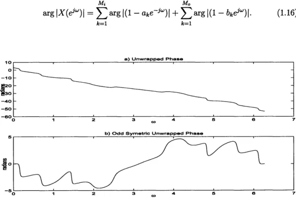
k=1 k=l1 a) Unwrapped Phase 1u 0 -10 E20 30 -40 -50 -60 _{I 1 2 3 .. 4 5 6 7}

b) Odd Symetric Unwrapped Phase

_5

A 0

-

--0 I 2 3 4 5 6 7

Figure 1-2: a) Example unwrapped phase function. b) Unwrapped phase function

without the linear phase and the contribution of the additive r constant.

I I I

1.3 Example Phase Functions

This section presents several examples of the wrapped and unwrapped phase

func-tions. The goal is to study how these functions vary with the locations in the z-plane

of the zeros of the z-transform of a signal.

Consider a real finite-length signal with one pair of conjugate zeros at angles 7r/4

& -7r/4 and radius r. The z-transform of this signal is

X(z)

=

(1

rej7/

re-j7/

z-1).

(1.17)

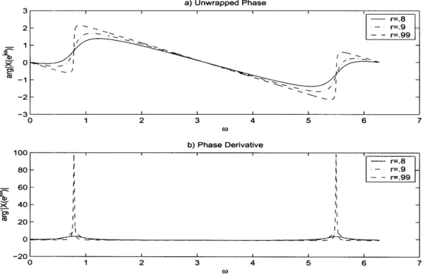
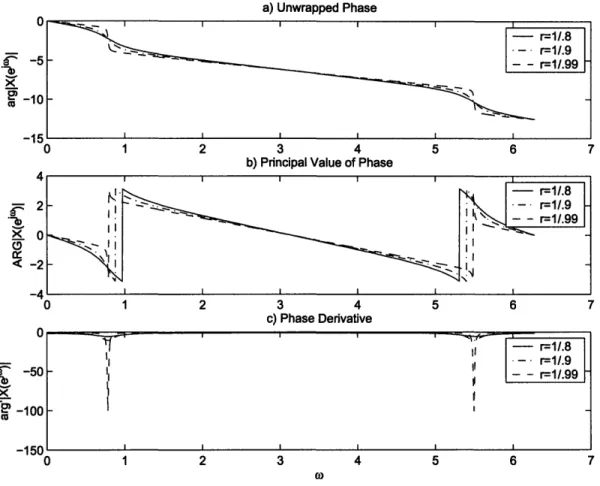
Figure 1-3 shows the unwrapped phase and phase derivative of X(ejw) for r = .8,.9, &.99. Note that in this case the unwrapped phase is equal to the principal value. a) Unwrapped Phase 2 -1 -2 N 'R 0 1 2 3 4 5 6 7 co b) Phase Derivative 100 r=.8 80 - r=.99 60 -0

-20

Figure 1-3: a) Unwrapped phase function. b) Phase Derivative.

Figure 1-4 shows the unwrapped phase with the contribution of the linear phase

component, the principal value of the phase, and the phase derivative of X(ejw) for

r

=

1

&

a) Unwrapped Phase U . -5

x

<:-2

x.

b) Principal Value of Phase

5 6 7

1 2 3 4 5 6 7

c) Phase Derivative

1 2 3 4 5 6 7

(0

Figure 1-4: a) Unwrapped phase function. b) Principal Value. c) Phase Derivative.

Figures 1-3 and 1-4 demonstrate that the closer the zeros of the z-transform are

to the unit circle the sharper the phase change at frequencies in their vicinity. These

sharp variations are the principle cause of the difficulty of phase unwrapping.

r=1/.8 r=1/.9 r=1/.99 - r=1/.8 _X t l| . r=1/.9 I - - r=1.99 I I I I I I I I A_ ::) 3 n I I I I 'O I

Chapter 2

Existing Algorithms to Compute

the Unwrapped Phase

When the complex cepstrum is computed, the discrete Fourier transform (DFT) is

used instead of the DTFT. The DFT is a sampled version of the DTFT, usually at

the roots of unity w = 27rk/N where k E Z and N E N.

k[k]

= X(ejkN)

= log IX[k] + j arg IX[k]l

Hence, only the corresponding samples of the unwrapped phase are needed. This

section will describe several existing algorithms to compute these samples.

2.1 Phase Unwrapping by Detecting

Discontinu-ities

The unwrapped phase can be obtained from the principal value of the phase, as

in equation 1.14, by detecting and removing the discontinuities introduced by the

arctangent routine. One way to implement this is by finding and removing differences

[1]. The algorithm starts by calculating A[k], the first difference of the samples of the principal value, using

A[k] = ARGIX[k + 1] - ARGIX[k]l. (2.1)

Next, any values of A[k] that lie outside the range [-7r, r[ get wrapped to obtain

WA[k] whose values lie within that range (L[k] is an integer function of k):

WA[k] = A[k] + 27rL[k] (2.2)

such that - r < WA[k] < 7r.

A correction sequence will be defined as:

CA[k] = WA[k] - A[k] = 2irL[k]. (2.3)

The unwrapped phase is then obtained by

k-1

arg IX[k + 1]1 = ARGIX[k + 1]1 + E CA[m].

(2.4)

m=O

The limitation of this method is that it only uses samples of the principal value

of the phase to perform the unwrapping. It also assumes that there is at most a

change of r in the unwrapped phase from one sample in frequency to the next. This assumption fails when the phase varies rapidly; the closer the zeros of the z-transform

of a signal are to the unit circle the more rapidly its DTFT phase varies. The ability

of this method to detect the 2r discontinuities is determined by the distance (2r/N)

between adjacent samples of the phase. This distance is controlled by N, the size of

the DFT; therefore, if the DFT size is too small relative to the variation of the phase

this method will fail to compute the correct unwrapped phase.

One possible way to check that the correct DFT size is chosen, is to compute the unwrapped phase using progressively longer DFTs until two consecutive unwrapped phase functions match, and assume that is the correct DFT size. An efficient

imple-mentation uses the FFT and increases the size by consecutive powers of two.

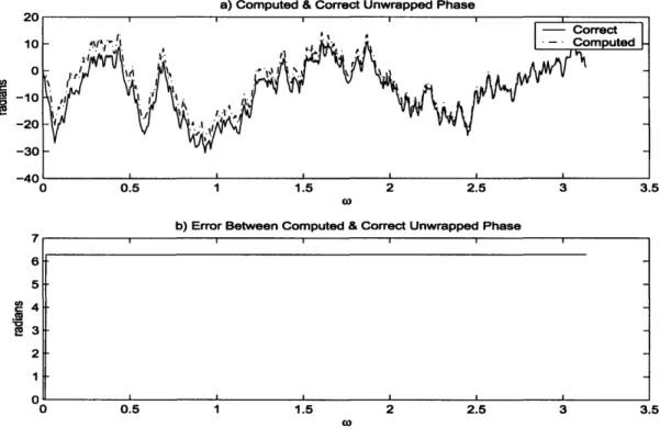
This method mainly fails in the following two situations: the first, is when a

match is not found before the maximum allowed (by the hardware) DFT size is

reached. The second, is when a match is found, but it is not the correct unwrapped

phase (i.e. an even larger DFT size would yield a different answer). An example of

the latter is shown in Figure 2-1, the unwrapped phases with DFT sizes equal to 214

& 215 matched; however, the correct unwrapped phase function requires a 216 DFT

size. Note that the linear phase components are different between the correct and the

computed phase functions, thus when they are removed the error between the two

functions is no longer limited to be a multiple of 27r as in Figure 2-1 (b).

In Cu co 0 t, ._ La

a) Computed & Correct Unwrapped Phase

0.5 1 1.5 2 2.5 3

co

b) Error Between Computed & Correct Unwrapped Phase

i i i i I 7. 6 5 4 3 2 1 0 0 0.5 1.5 2 2.5 co 3 1 3.5 3.5

Figure 2-1: a) Correct and computed unwrapped phase functions after removal of

linear phase component. b) Error in the correct and computed unwrapped phase

(before removal of linear phase component).

2.2 Phase Unwrapping Using Adaptive Numerical

Integration

Equation (1.15) suggests that samples of the unwrapped phase can be obtained by

numerical integration of samples of the phase derivative. The accuracy of the nu-merical integration will be limited by the integration step size, which is the distance between adjacent samples. Unfortunately, it does not seem possible to determine a

priori the DFT size needed to obtain a correct unwrapped phase function.

Tribolet [4] suggested an adaptive numerical integration method. He assumed that the value of the unwrapped phase at the frequency sample wk is known, and used the

trapezoidal rule to perform the numerical integration and obtain an estimate of the

unwrapped phase at wk+l:

afglX[wk+l]I = arg IX[wk] + Wk+l - wk

{arg'

(2.5)

2

However, depending on the step size (k+1 - Wk), the obtained value aglX[wk+l]l

may be inconsistent relative to ARGIX[wk+ll]l. The calculated value is assumed

in-consistent when:

IagX[wk+1]I - ARGIX[wk+1]I + 2irl[wk+1]I > e, (2.6)

where 1[Wk+l] is an integer and E is a set threshold. If the calculated value of aiglX[wk+llI

is

Equa-tions (2.5) and (2.6) are then repeated until a consistent estimate of the unwrapped

phase is obtained. The unwrapped phase at sample wk+1 is then computed by:

arg IX[wk+1]l = ARGIX[wk+l]I + 27rl[wk+l] (2.7)

This method becomes less appealing the closer the zeros of the z-transform of the

signal are to the unit circle. As was observed in Section 1.3, the closer a zero is to the

in consequence the smaller the integration step size needs to be. The smaller step size

is obtained by repeated iterations of the step size adaptation. Hence, this algorithm

will become more computationally intensive as more of the zeros of the z-transform

of the signal approach the unit circle.

An issue of greater concern with this method is that a false yet consistent (accord-ing to (2.6)) estimate of a sample of the unwrapped phase could be obtained, caus(accord-ing the calculated unwrapped phase to be incorrect. Using a smaller threshold £ will

most likely yield a more accurate unwrapped phase. However, this would increase the

number of step size adaptations. It is important to note that there is no guarantee

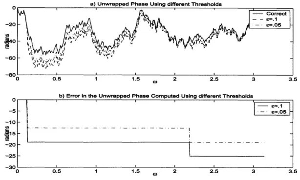
that an even smaller step size would not yield a different unwrapped phase function. Figure 2-2 shows an example that clearly highlights these issues. Consider cal-culating samples of the unwrapped phase of a signal of length 1024 using adaptive numerical integration. Three different thresholds are used: = .1, .05, &.01. Of these only E = .01 yields the correct unwrapped phase. As can be seen in the figure the

higher thresholds yielded erroneous unwrapped phase functions with the errors equal

to multiples of 2. It is also important to note that a threshold of .1 required 2673

iterations of the step size adaptation, while

= .05 required 3207 and

= .01 required

5245. These numbers clearly show the inverse relationship between the value of the

threshold and computational intensity; in our implementation of this algorithm we

used E = .05.

A modification to this method presented by Scott [5] uses the phase derivative at

the two endslopes (arg' IX[wk+l]l & arg' IX[k]l

I)

integra-tion along with their average to improve the confidence of the algorithm.

Another modification [6] to the adaptive integration method used the second

deriva-tives of the phase (arg" IX(ejw)I) to perform piecewise polynomial interpolation using cubic splines, as a substitute to the trapezoidal integration used by Tribolet.

0 -20 -640 -60 -An 0 0.5 1 1.5 2 2.5 3 3.5 0 -5 -10 -20 -25 -30 0 0.5 1 1.5 2 2.5 3 3.5

Figure 2-2: a) Unwrapped phase function after removal of linear phase component for

different thresholds. b)Error in the computed unwrapped phase for different

thresh-olds.

2.3 Computation of the Unwrapped Phase Using

Polynomial Factoring

Steiglitz and Dickinson [7] suggested calculating the roots of the polynomial

(z-transform) of a finite length signal. The unwrapped phase is then obtained by adding

together the phase contributions of each root, as in Equation (1.16). The success of

this method depends on the success of the polynomial factoring algorithm used to

calculate the roots.

A new efficient method for factoring high degree polynomials was proposed by

Sitton and Burrus [8]. The method uses the Fast Fourier Transform (FFT) to create

a search grid around the unit circle by evaluating the z-transform of the signal at

evenly spaced samples on concentric circles with radii close to 1 in the z-plane (see Figure 2-3).

Figure 2-3: A depiction, reproduced from [8], of a sample search grid.

and then Newton's method [9] is used to obtain the exact locations of the zeros. This

polynomial factoring algorithm focuses on searching for zeros in the area close to the

unit circle, and thus works better on polynomials with zeros clustered closer to the

unit circle. However, this factoring method becomes less efficient and is more likely to fail on signals for which the zeros of their z-transforms are farther from the unit circle,

and in such cases the correct unwrapped phase cannot be obtained from the factored

roots. A detailed explanation of this polynomial factoring algorithm is provided in

the next chapter.

2.4 Phase Unwrapping from the Time Series

McGowan [13] presented a method that uses the discrete-time sequence x[n] to

deter-mine the additive factor required at each sample in frequency to unwrap the phase.

The algorithm is based on finding the integer-valued function l(Wk+l) in the following

equation:

arg[X(ejk+l)] - arg[X(eJwk)]

=

-{arctan[XI

j,

+

rl(wk+i)}.

(2.8)

In this case, the arctan routine used returns a value for the phase between -r/2

and 7r/2. The term

is found by tracking how many times the sign of

XR(eJ-)

changes as w goes through a singularity of the ratio or similarly the change in sign of Xi(ej") XR(ej ) as w goes through the zeros of XR(ejw). For example, as w

goes through a zero of XR(ej ' ) and the sign of XI(ej") ·XR(e" j ) changes from +ve

to -ve, 1(Wk+1) is incremented by one and it is decremented by one as the sign of

XI(eJi).XR(e jw)

goes from -ve to +ve. To calculate the number of sign changes

l(wk+l)

at each

the discrete-time sequence and Sturm Polynomials [14] are used.

This method unwraps the phase at any frequency directly from the time series

without the need to obtain the unwrapped phase of any intermediate values. Also

the unwrapped phase at a certain frequency can be obtained from a fixed number

of calculations. However, a major limitation of this method is that it is restricted

to extremely short time sequences. An improvement on this method, that allows

for longer time sequences, was presented by Long [15]. This improvement, however, becomes less accurate as the signal length increases due to computational errors.

2.5 Iterative Method to Compute the Unwrapped

Phase

This method proposed by Quatieri and Oppenheim in [17] computes the unwrapped

phase of the DTFT of an input x[n] in the following steps:

1. Iterative techniques are used to compute a minimum-phase sequence Xmp[n]

from the principal value of the phase of the mixed-phase input sequence x[n] with the linear-phase component removed.

2. The log of the magnitude of the DTFT of the minimum-phase sequence log IX(eJw)l is then used to compute the unwrapped phase arg IXmp(eJi)l of xmp[n] using the

Hilbert transform relationships [2] of minimum-phase sequences.

3. The unwrapped phase arg IX(ejw)l is then obtained by adding the linear-phase

component removed in step 1 to arg IXmp(eiw)l.

This was successfully tested in [17] on simple mixed-phase sequences. However, no results are presented in [17] for long sequences and it suffers from several compli-cations. Specifically, xmp[n] is infinite in length even if x[n] is finite length; therefore,

the DFT size used in the iteration needs to be large enough to ensure aliasing will

not occur. Another issue with this algorithm is that it requires the linear phase

component of the phase of x[n] to be known a priori which is in general not the case.

2.6 Phase Unwrapping by Isolating Sharp Zeros

The method presented in [18] uses the locations of the zeros of the signal that are

close to the unit circle to compute the unwrapped phase. The method attempts

to determine the radial positions of sharp zeros within segments of the z-plane. A

segment is the frequency step between two consecutive samples of the DFT (27r/N). Sharp zeros as defined in [18] are ones that are close to the unit circle, particularly whose radii are between .99 and 1.01. A zero is in a segment if it lies between the

two radial lines that pass through the DFT sample points and extend to infinity. The

algorithm develops and uses two measures to obtain the radial positions:

1. Phase derivative with respect to radial distance, which is the derivative with

respect radial distance of the phase change across a segment.

2. Phase derivative at any frequency sampling point k with respect to radial

dis-tance.

Once the radial positions of the sharp zeros within a segment are computed, they

are used to determine the theoretical phase change across that segment. This is

then compared to the change in the principal value over that segment to obtain the

appropriate multiple of 27r required to unwrap the phase.

This method performs well provided the signal does not have many sharp zeros clustered close to each other. When such clustering occurs a sharp zero might be missed resulting in a false unwrapped phase.

2.7 Summary

Of the methods presented in this section only the first three are of particular interest

to us. Phase unwrapping by detecting discontinuities (DD) and by adaptive numerical

integration (ANI) are the most widely used methods, and recent advances in poly-nomial factoring [8] have made computation of the unwrapped phase by polypoly-nomial

factoring (PF) a more attractive method.

Both DD and ANI assume that there is a limit to how fast the unwrapped phase

may vary in frequency. However, Section 1.3 demonstrated that the unwrapped phase

has sharp variations near zeros that are close to the unit circle. Therefore, these

meth-ods will perform poorly on signals that have most of their z-transform zeros clustered near the unit circle. The polynomial factoring algorithm presented in [8] is capable of factoring high degree polynomials whose zeros are located close to the unit

cir-cle. Thus, using this factoring algorithm in PF leads to correct computation of the

unwrapped phase for signals that cause DD and ANI to perform poorly. The fact

that PF is complementary to both DD and ANI motivates the proposed composite

methods presented in Chapter 4.

Chapter 3

Method for Factoring High Degree

Polynomials

In [7] a new method for factoring high degree polynomials was presented that can factor polynomials with random coefficients with degree as high as a million. This

algorithm uses the property that zeros of polynomials with random coefficients cluster

in an annulus around the unit circle, and the area of the annulus gets smaller as the

degree increases, as presented in Appendix A. This property allows the algorithm to

focus the search for zeros in the vicinity of the unit circle.

3.1 Outline of the Algorithm

1. A search grid that is dense near the unit circle is created by sampling the z-plane at concentric circles. This is done by expanding and contracting the z-plane (by

applying an exponential weighting to the input) and then computing its FFT.

2. The grid is searched for local minima. These present candidate locations for the zeros of the signal.

3. The candidate locations from step 2 are then polished using Newton's [9] or

method is quadratic, while that of Laguerre is cubic.

4. If the search missed some roots then the computed roots are used to deflate the

original polynomial to obtain one of lower degree.

5. The deflated polynomial is then factored, and the newly found roots polished against the original polynomial.

6. Ideally steps 4 and 5 are repeated until all roots are found. However, the deflation process is highly prone to errors. When deflation fails, the algorithm

returns to step 1 and searches over a denser grid.

3.2 Deflation Failure

One of the major sources of error in this polynomial factoring algorithm, is the

de-flation step. Dede-flation errors usually happen when either the input polynomial is

ill-conditioned or the resulting deflated polynomial is ill-conditioned, i.e. one for which a slight change in the coefficients results in a large change in the zero locations. Below is an example of deflation failure. This example is taken from the authors of

this factoring algorithm.

Consider a well conditioned polynomial of degree 1000 with coefficients drawn from a zero mean independent identically distributed uniform distribution. Assume the grid searching and polishing found 986 of the 1000 zeros of the z-transform of the signal. Moreover, assume the remaining 14 zeros are located near z = 1 in the z-plane, as shown in Figure 3-1(a).

The zeros found are then used to deflated the original polynomial. The resulting

fourteenth degree polynomial has zeros that are plotted in Figure 3-1(b). Comparing these zero locations to the ones in Figure 3-1(a) shows that the deflation failed.

a) Z-plane plot of correct location of remaining zeros c - _u0.5 E -1 -3 -2 -1 0 1 2 3 Real Part

b) Z-plane plot of the location of the zeros of the deflated polynomial

.'0

0

Figure 3-1: a) Z-plane plot showing the correct location of the remaining 14 zeros. b) Z-plane plot showing the zero locations of the deflated polynomial.

3.3 Discussion

This factoring algorithm focusses its search for zeros in the vicinity of the unit circle.

Hence, this algorithm performs well on polynomials with zeros that cluster in a tight

annulus around the unit circle. Appendix A shows that polynomials with coefficients

that are i.i.d. random variables exhibit this property. Moreover, this property also

holds for polynomials whose coefficients are samples of naturally occurring physical signals such as speech and Electroencephalography (EEG). However, when the

as-sumption of the zeros clustering around the unit circle does not hold, this method

will perform poorly and may even fail to factor the polynomial. Another case where this method could fail is when the input polynomial is ill-conditioned.

Chapter 4

Proposed Composite Methods

This chapter will present two new methods for phase unwrapping that are capable of

reliably computing the unwrapped phase in situations where the existing algorithms

may fail.

4.1 Motivation

Phase unwrapping by detecting discontinuities (DD) presented in Section 2.1 and

phase unwrapping by adaptive numerical integration (ANI) presented in Section 2.2

are the most frequently used in practice. These methods become inefficient and

may fail as the zeros of the z-transform of the signal approach the unit circle. This

limitation is of concern because, as was presented in Appendix A, sampled natural

physical signals tend to have their zeros clustered in a tight annulus around the unit

circle. Moreover, the area of the annulus decreases with increasing signal size. On the

other hand, computation of the unwrapped phase by polynomial factoring (PF) using

the algorithm presented in Chapter 3 performs best when all the zeros are close to

the unit circle. Consequently, we conclude that the DD and ANI methods tend to be

complementary to the PF method: DD and ANI perform poorly when PF performs

well and vice versa. This motivates an algorithm that uses polynomial factoring with

4.2

Overview

The proposed composite methods consider any signal x[n] as a convolution of two signals xuc[n] and x,em,[n].

x[n] = ,.emf[n]

* xuc[n] & X(z) = X,,m(z)XUc(z)

(4.1)

Xuc(z) contains the zeros of X(z) that are problematic for DD and ANI, i.e. zeros

that are closer to the unit circle (zuc), and X,,m(z) contains the remaining zeros of

X(z).

The proposed algorithm is a five step process:

1- Use polynomial factoring to find the zeros that are clustered near the unit circle,

i.e. zeros of Xuc(z).

2- Calculate the unwrapped phase contribution (arg Xuc(eJ'w)) of these zeros.

3- Obtain xrem[n] by deconvolving xuc[n] from x[n].

4- Use either the DD or ANI algorithm to unwrap the phase contribution of the

remaining zeros to get arg IXrem(eji)

I.

5- Add the unwrapped phase calculated in step 2 and in step 4 to obtain the total

unwrapped phase.

arg IX(e) = arg Xuc(ei")l + arg IXrem(ejiw) (4.2)

This five step process is a simplification of the actual proposed algorithm, and

assumes that xrem[n] can correctly be calculated by deflation. However, this is in many cases not true; therefore, step 4 cannot be directly applied. Modifications are

made to the DD and ANI methods to accomodate these cases. These modifications

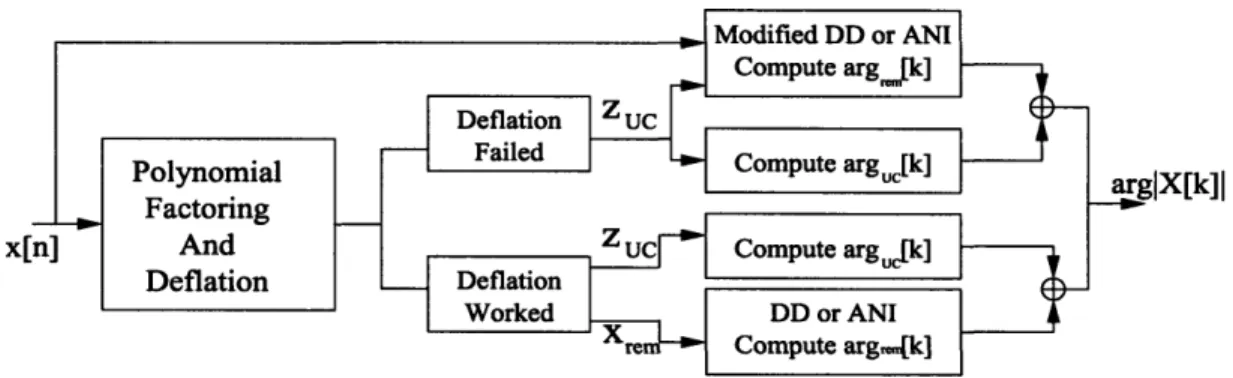
require the original signal x[n] and zuc as inputs. Figure 4-1 is a block diagram

representation of the proposed algorithms. The next sections of this chapter will

describe the details of the polynomial factoring part, and those of the modified DD

and ANI algorithms.

xl

Figure 4-1: Overview block diagram.

4.3 Polynomial Factoring and Deflation

The concepts of polynomial factoring and deflation in the algorithm are taken from

Sitton and Burrus [8]. MATLAB code downloaded from the website [11] of the authors

of [8] was modified and used to implement this part of the algorithm.

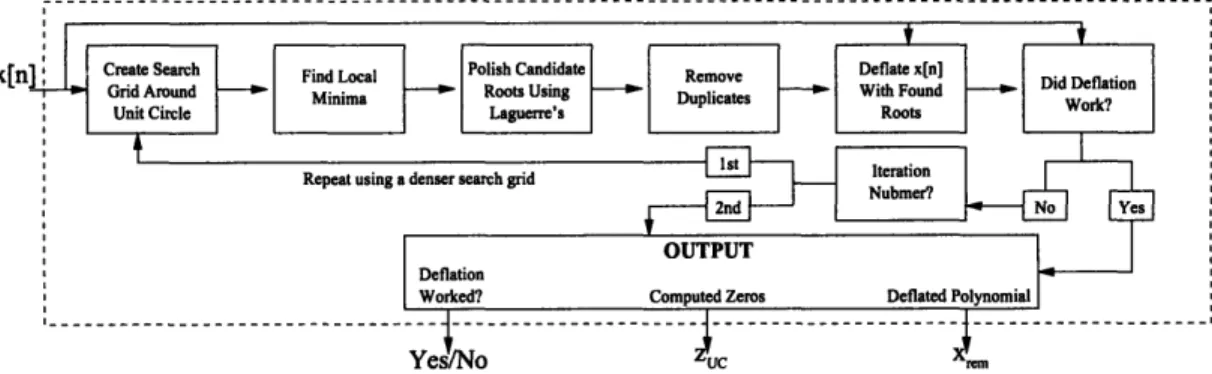
4.3.1

Steps to Find Zeros Close to the Unit Circle

This section briefly outlines the process used to search for zeros of the z-transform of a signal that are close to the unit circle.

1. Create a search grid that is dense around the unit circle.

2. Find local minima, and use them as candidate locations for roots.

3. Polish the candidate locations using Laguerre's algorithm to obtain the correct

location.

4. Remove any duplicates (zeros that polished to the same location) from the set

of computed zeros.

5. Deflate the input polynomial using the computed roots.

6. (a) If deflation worked, output the computed zeros and the deflated

polyno-mial, Xrem [n].

(b) If deflation failed, and this is the first iteration through these steps, repeat

(c) If deflation failed, and this is the second iteration, output the computed

zeros.

Our experience showed that a max of two iterations should be allowed to attempt

to obtain a deflated polynomial because a third iteration increases computation time

and in most cases does not help. It is important to note that this section of the

algorithm finds most of the zeros that are close to the unit circle, but will usually

miss a few: this is mainly because the signal may have multiple zeros that are very close to each other.

A block diagram outlining these steps is shown in Figure 4-2. The following sec-tions will describe in detail how the search grid was created, and how the polynomial deflation was performed.

- - - -..

Figure 4-2: Polynomial factoring and deflation block diagram.

4.3.2 Search Grid

The search grid is created by sampling the z-plane on concentric circles of varying

radii. This sampling is performed by applying exponential weighting to the input

sequence and then taking the DFT of the weighted sequence. Applying exponential

weighting to a signal refers to a pointwise multiplication of the signal with a positive

sequence a

'x

[n].

Taking the DFT of xep,[n] is equivalent to sampling the z-transform of x[n] at a radius

c-1:

Xexp(e

)

=

E x[n](a-leik)-n

X(

e

The grid is chosen so that it is denser near the unit circle: as the unit circle is approached the concentric circles are more closely spaced and the number of samples

(size of DFT) on each of the circles increases. A sample search grid is shown in Figure

4-3.

As is shown in the figure, the search grid only spans the inside of the unit circle. To

Example Search Grid Only Upper Right Quadrant Shown

'¥.f;.r~rf'~r. .r.g.r ...

- I

-0 0.1 0.2 0.3 0.4 0.5

Real

0.6 0.7 0.8 0.9 1

Figure 4-3: Sample search grid, only upper right hand quadrant shown.

0.9 0.8 0.7 0.6 'n 0.5 E 0.4 0.3 0.2 0.1 (4.3) . . . . : : J. _ _ . -I I I · I_

obtain samples on concentric circles outside the unit circle the time-reversed signal

x[-n] is used. A zero zo of x[-n] corresponds to a zero z' of x[n] [1] because

z-transform{x[-nJ] = X(1/z).

The goal of the grid search is to find candidate locations of zeros that are close to the unit circle. However, as is observed in Figure 4-3 the choice of grid covers the whole of the inside of the unit circle. The reason for this is that restricting the search to an area around the unit circle does not considerably speed up the algorithm (since the grid becomes sparse away from the unit circle). Also our experience showed that not restricting the grid found more zeros which led the deflation step to be more likely to succeed. In general, the majority of the candidate locations found by the grid correspond to zeros that are close to the unit circle.

4.3.3 Deflation

The deflation step attempts to obtain a polynomial xrem[n] of lower degree by

remov-ing the contributions of the computed zeros from the input polynomial. The deflation

separates the computed zeros into two different groups: those that are close to the

unit circle, and those that are not. The zeros far away from the unit circle are un-factored into a polynomial xfar[n] which is then used to deflate x[n] and obtain and intermediate polynomial i[n]; this deflation is carried out in the frequency domain using point-wise division

X[k] = X[k]/Xfar[k].

The zeros close to the unit circle are unfactored to form a polynomial xclose[n] which is then used to deflate x[n] and obtain xrem[n]; this deflation is done as a time domain

To check if deflation has worked, a polynomial x,re[n] is formed as

Xrec [n] = Xrem [n] * Xfar [n] * Xdose [n],

and compared to the input polynomial x[n].

4.4 Modified DD and ANI Algorithms

When deflation fails,

cannot be obtained. Thus, the DD and ANI algorithms

cannot be directly applied. This section shows how these algorithms can be modified

to compute arg

IXrem[k]

, without access to

using only the input signal

and the computed roots Zuc.

4.4.1 Modified DD Algorithm

To apply the DD phase unwrapping algorithm all that is needed are samples of the

wrapped phase ARGIX,m[k]l of xrem[n] (refer to Section 2.1). ARGIXrem[k]I can be computed by the following steps:

1. Compute ARGIX[k]I, samples of the wrapped phase of x[n], using the

arctan-gent routine.

2. Compute arg IXuc[k]l from the computed roots zuc by summing the individual

phase contributions of each zero.

3. Subtract modulo 27r the unwrapped phase of the computed roots from the

wrapped phase of the input x[n],

4.4.2 Modified ANI Algorithm

In ANI (Section 2.2) samples of the wrapped phase ARGIXrem[k]I and samples of the phase derivative arg' IXrem[k]

I

how ARGIXrem[k][ can be computed. Similarly, arg' Xrem[k]l can be computed in the following steps:

1. Compute arg' IX[k]l, samples of the phase derivative of x[n], using

arg'IX[k]l =

Xk]

}-2. Compute arg' IXvc[k] I from the computed roots zuc by summing the individual

phase derivative contributions of each zero.

3. Subtract the phase derivative of the computed roots from the phase derivative of the input x[n],

arg' IXrem[k]l

= arg' X[k]I - arg' IXuc[k].

This algorithm also requires that the step size be reduced when the numerical

inte-gration fails to produce consistent results (Section 2.2). With each step size reduction

a new sample of ARGIXrem(eiw)l and arg' IXrem(ej") is required. This can be done using the same steps described above for one DFT point.

4.5 Robustness To Errors In Factored Zeros

The polynomial factoring part of the algorithm also computes an estimate of the error of each polished root. The error estimate, as proposed in the code obtained from [11], is based on the Newton correction -f(z)/f'(z) evaluated at the location of the polished zero. Errors incurred by the polynomial factoring section of the algorithm may cause the deflation to fail; however, in general they will not translate into errors

To see this, consider a signal x[n] with the following z-transform and unwrapped

phase

X(z)

arg IX(ej )I

=

Xrem(z)(1 - zoz

)

= arg IXrem(ej) + argl (1- ze-j)l.

We assume that the polynomial factoring algorithm erroneously computed a zero at

Z, instead of z. Therefore, the wrapped phase and the phase derivative of the input

deflated by the computed root are

ARGIXrem(ew)Il = ARGIXrem(e3j)I + ARGI(1 - ze-j)l - ARGI(1 - ioe-j3)l

and

arg' IXrem(ejw)l = arg' IXrem(ejW)I + arg' 1(1 -

zoe-j)l-

Performing the unwrapping of ARGIXem(ejw)l using either the modified DD or the

modified ANI algorithms yields:

arg IXrem(ejW) = arg IXr,(ejW)l + argl(1 - zoe-j)

arg 1(1 -

oe-jw)l.

Finally, combining the unwrapped phase of the found roots with that of Xrem(e

_w)

gives the unwrapped phase of X(ejw):

arg IX(eJW)l

= arg IXrm(e)l + arg 1(1

e-j)

= arg IXe(ejW)l + arg (1

zeJwl-

arg l(1

o-jw)l

+arg

aoe-j~)l

l(1

-= arg IXrem(ejw)l + arg 1(1 - z(e-j)I (4.7)

Thus, we have shown that an error in a zero location due to the first section

of the algorithm will be absorbed into the second section as the phase contribution

of a pole, and will not affect the final computed unwrapped phase. It is important

(4.5)

to note, however, that if the errors are large they will interfere with the DD and ANI algorithms; therefore, zeros whose errors estimates are large are removed. Our experience has led us to remove zeros whose estimated errors were larger than 10-6.

4.6 Summary

The two proposed composite algorithms for computing the unwrapped phase ex-ploit the fact that PF is complementary to DD and ANI. PF favors signals whose z-transform zeros are tightly clustered near the unit circle. DD and ANI favor signals whose z-transform zeros are located far from the unit circle. By combining these algorithms it is possible to unwrap the phase of most mixed-phase input signals, re-gardless of the distribution of their zeros.

The first proposed composite algorithm (CA) combines polynomial factoring

(Section 4.3) with phase unwrapping by detecting discontinuities (Section 2.1). The

second proposed composite algorithm (CA2) combines polynomial factoring with phase unwrapping by adaptive numerical integration. CA2 is more accurate than CA1 due to the consistency test in ANI (Section 2.2); in our implementation of CA2 the threshold in the consistency test is chosen to be e = .05.

The next chapter presents experimental results that demonstrate the superiority

Chapter 5

Algorithm Evaluation

This chapter presents experimental results that demonstrate the superiority of the

proposed composite algorithms over the existing methods. We compare phase

un-wrapping by detecting discontinuities (Section 2.1), phase unun-wrapping by adaptive

numerical integration (Section 2.2), phase unwrapping by polynomial factoring

(Sec-tion 2.3), and both proposed composite algorithms CA1 and CA2 . The criterion for

comparison is both speed and accuracy. The signals that are used to evaluate these

algorithms are:

1. A synthetic signal with z-transform zeros that are clustered near the unit circle.

2. A synthetic signal with z-transform zeros that are away from the unit circle. 3. A synthetic signal with z-transform zeros that are both close to and far away

from the unit circle.

4. A large number of synthetic signals with z-transform zeros whose locations are randomly chosen in the z-plane.

5. Sampled physical signals, specifically speech and EEG signals. 6. Filtered speech and EEG signals.

For the first three synthetic signals and the sampled physical signals a table will be

used to summarize the performance of the different phase unwrapping algorithms.

The table consists of the following:

1. Whether the algorithm correctly computes the unwrapped phase.

2. Run time of a MATLAB implementation of the algorithm on a PC with a

1.6GHz Pentium M processor and 512 MB of RAM. 3. Additional relevant details:

(a) Number of step size adaptation iterations required to unwrap the phase of

x[n] and x,em[n] in ANI and CA2 respectively.

(b) Size of DFT used to unwrap the phase of x[n] and rem,,[n] in DD and CA1

respectively.

Our evaluation using the large number of synthetic signals is based on the average

run time of the algorithms and percentage of times the algorithms correctly computed

the unwrapped phase.

In this thesis we only consider real-valued signals; however, with minor modifi-cations the algorithms perform in a similar fashion when applied to complex-valued

input signals.

5.1 Algorithm Evaluation Using Synthetic Signals

This section uses synthetic signals to compare the different phase unwrapping

algo-rithms. Since we generate the data, the exact locations of the roots are known and

therefore from Section 2.3 the correct unwrapped phase can be computed and used to check the different algorithms. The locations of the zeros are chosen to evaluate algorithm performance for three main classes of signals:

1. signals with z-transform zeros that cluster near the unit circle.

2. signals with z-transform zeros that lie far away from the unit circle.

3. signals with z-transform zeros that are located both close to and away from the

We also evaluate the performance using a large number of synthetic signals whose

zero locations are randomly chosen to span these classes.

The synthetic signals are generated as a convolution of several exponentially weighted random real coefficient (either uniformly or normally distributed) signals. As is presented in Appendix A zeros of polynomials with random coefficients are

clus-tered in a tight annulus around the unit circle. Applying exponential weighting to

a sequence (4.3.2) changes the center radius of the annulus. Therefore, the zeros of the z-transform of the generated synthetic signals are in concentric annuli of varying

center radii.

5.1.1 Synthetic Signal with Zeros Close to the Unit Circle

We generate a signal, of length=4093, with z-transform zeros concentrated in annuli

with center radii of: 1,.9999 & 1/.9999. Figure 5-1 (a) shows the histogram of the

distribution of the radii the zeros.

10 5

1!

-5

-10

a) Histogram of radii of zeros

0 0.5 1 1.5

radius

b) Correct unwrapped phase of signal with zeros close to the unit circle

-150 L

0 1 2 3 4 5 6 7

Figure 5-1: Results for the synthetic signal with zeros close to the unit circle.

2

7

IOu

Method Correct Run Time Details

DD No 0.5sec DFT size used N=23 2

ANI Yes 86.83sec Number of step size adaptations=11572 PF Yes 49.6sec Factoring worked

CA1 Yes 17.47sec DFT size used N=213

CA2 Yes 45.8sec Number of step size adaptations=105

Table 5.1: Results for the synthetic signal with zeros close to the unit circle.

As we see from Table 5.1 PF works well, while DD and ANI perform poorly. Specifically, DD fails, and even though ANI correctly unwraps the phase it is highly

inefficient, requiring 11572 step size adaptations and 87 seconds to run. On the other

hand, in CA2 the polynomial factorization finds and removes most of the zeros close to

the unit circle. Therefore, the phase contribution of the remaining zeros is unwrapped

using only 105 step size adaptations.

5.1.2 Synthetic Signal with Zeros Far from the Unit Circle

We generate a signal, of length=4093, with z-transform zeros concentrated in annuli

with center radii of: .9,.8 & 1/.9. Figure 5-2 (a) shows the histogram of the

distribu-tion of the radii of the zeros.

Method Correct Run Time Details

DD Yes 0.1sec DFT size used N=24

ANI Yes .2sec Number of step size adaptations=0

PF

No

N/A

Factoring failed

CA1 Yes 1.92sec DFT size used N=21 3

CA2 Yes 2.1sec Number of step size adaptations=0 Table 5.2: Results for the synthetic signal with zeros far from the unit circle.

As we see from Table 5.2 DD and ANI correctly and efficiently unwrap the phase. Specifically, ANI requires no step-size adaptation and calculates the correct phase in only .2 seconds. This signal also shows an example where PF fails to factor the signal.

a) Histogram of radii of zeros

, . ..

) 0.5 1 1.5 2 2.

radius

b) Correct unwrapped phase of signal with zeros away from the unit circle

10 5 0 -5 -10 -15 C 1 2 3 co 4 5 6

Figure 5-2: Results for the synthetic signal with zeros far from the unit circle.

5.1.3 Synthetic Signal with Zeros Close to and Far from the

Unit Circle

We generate a signal of length=4093, with z-transform zeros concentrated in annuli

with center radii of: 1, .9, .999, & 1/.9. Figure 5-3 (a) shows the histogram of the

distribution of the radii of the zeros.

I

Method Correct Run Time Details

DD No 0.57sec DFT size used N=232

ANI Yes 43.27sec Number of step size adaptations=8398

PF

No

N/A

Factoring failed

CA1 Yes 8.02sec DFT size used N=2 13

CA2 Yes 30.5sec Number of step size adaptations=56 Table 5.3: Results for the

circle.

synthetic signal with zeros close to and far from the unit

This synthetic signal illustrates a case where the existing algorithms perform

poorly. Specifically, Table 5.3 shows that DD and PF fail, while ANI requires 8398

step size adaptations to correctly unwrap the phase. In this example the advantage

dUU 1500 1000 500 15

II