Winding Roads: Routing edges into bundles

(1)

HAL Id: hal-00495279

https://hal.archives-ouvertes.fr/hal-00495279

Submitted on 25 Jun 2010

HAL is a multi-disciplinary open access

archive for the deposit and dissemination of

sci-entific research documents, whether they are

pub-lished or not. The documents may come from

teaching and research institutions in France or

abroad, or from public or private research centers.

L’archive ouverte pluridisciplinaire HAL, est

destinée au dépôt et à la diffusion de documents

scientifiques de niveau recherche, publiés ou non,

émanant des établissements d’enseignement et de

recherche français ou étrangers, des laboratoires

publics ou privés.

Winding Roads: Routing edges into bundles

Antoine Lambert, Romain Bourqui, David Auber

To cite this version:

Antoine Lambert, Romain Bourqui, David Auber. Winding Roads: Routing edges into bundles.

Computer Graphics Forum, Wiley, 2010, 29 (3), pp.853-862. �hal-00495279�

(2)

Eurographics/ IEEE-VGTC Symposium on Visualization 2010 G. Melançon, T. Munzner, and D. Weiskopf

(Guest Editors)

Volume 29(2010), Number 3

Winding Roads: Routing edges into bundles

A. Lambert and R. Bourqui and D. Auber

CNRS UMR5800 LaBRI, INRIA Bordeaux - Sud Ouest, France

Abstract

Visualizing graphs containing many nodes and edges efficiently is quite challenging. Drawings of such graphs generally suffer from visual clutter induced by the large amount of edges and their crossings. Consequently, it is difficult to read the relationships between nodes and the high-level edge patterns that may exist in standard node-link diagram representations. Edge bundling techniques have been proposed to help solve this issue, which rely on high quality edge rerouting. In this paper, we introduce an intuitive edge bundling technique which efficiently reduces edge clutter in graphs drawings. Our method is based on the use of a grid built using the original graph to compute the edge rerouting. In comparison with previously proposed edge bundling methods, our technique improves both the level of clutter reduction and the computation performance. The second contribution of this paper is a GPU-based rendering method which helps users perceive bundles densities while preserving edge color.

Categories and Subject Descriptors (according to ACM CCS): I.3.3 [Computer Graphics]: Picture/Image Generation—Line and curve generation

1. Introduction

Graphs play an important role in many research areas, such as biology, microelectronics, social sciences, data min-ing, and computer science. Improvements in data acquisition techniques drive the need for visualization, as the size and the complexity of acquired graphs prohibit manual draw-ing. The graph drawing and information visualization com-munities focus on designing effective visualizations of such large graphs. For particular classes of graphs, such as trees, planar graphs or directed acyclic graphs, effective solutions have been found that give very good results ; not only in terms of time and space complexity but also in terms of aes-thetic criteria. However, real-world graphs from application domains usually do not belong to these classes. To find an algorithm that gives good results (in terms of computation time, aesthetic criteria and information emphasized) for ar-bitrary graphs is a difficult problem. As it produces visually pleasant and structurally significant results, the most pop-ular approaches to draw such graphs are the force-directed approaches (e.g., [FLM94,HJ04]).

However, due to data complexity, we cannot expect force-directed approaches to give readable representations of all

graphs. To the best of our knowledge, there exists for in-stance no drawing algorithm that offers a satisfying layout of a scale-free network (i.e. a graph whose degree distribu-tion follows a power law). Furthermore, in some applica-tion domains, such as geography, nodes posiapplica-tions cannot be changed as they bring information. In such cases, informa-tion discovery becomes difficult as edge crossings and node-edge overlaps clutter the representation. Reducing the clutter in a graph representation is therefore of utmost importance to identify relationships and high-level edge patterns.

In the past, clutter reduction had been achieved using two main techniques : compound visualization and edge bundling. In a compound visualization (e.g [vv04,AvK06,

AMA07]), an abstraction of the original network is built by collapsing clusters into metanodes and the result is then displayed on the screen. This technique reduces the clutter-ing of the representation as inter-cluster edges are merged into metaedges. However, complex interactions for collaps-ing/expanding metanodes are necessary to retrieve the in-formation. Furthermore, the compound visualization is not suitable when nodes positions cannot be changed as clusters may overlap.

(3)

Recently, edge bundling techniques [PXY∗₀₅_,_Hol06_,

CZQ∗₀₈_,_Hv09_{] are of increasing interest in the graph}

visualization community. Put under the spotlight by Holten [Hol06], this technique routes edges into bundles in order to uncover high level edge patterns and to emphasize relationships in relational data.

In this paper, we focus on a novel approach to gener-ate edge-bundled representations of graphs. We introduce an intuitive edge bundling algorithm which efficiently reduces edge clutter in graphs drawings. Our method discretizes the plane into regions. Boundaries of these regions are used as

roadsto route edges. The main contribution of this paper is therefore a new edge bundling technique that improves com-putation times when compared to existing methods but also avoids node-edge overlaps. The second contribution of this paper is a GPU-based rendering method which enables users to perceive bundle densities while preserving edge color. Our algorithm and rendering technique have been imple-mented as two plugins for the Tulip graph visualization soft-ware [Aub03].

The remainder of this paper is structured as follows. Sec-tion2reviews related work on edge clutter reduction meth-ods and techniques to enhance edge bundles visualization. In section3and4, we present the main steps of our method and several implementation issues. We next explain a way to parametrize the level of clutter reduction in section5. Sec-tion6refers to rendering techniques necessitated by edge bundling visualization. Finally, we draw a conclusion and give directions for future work in section7.

2. Previous Work

As mentioned above, we focus in this paper on a repre-sentation of edges whose extremities have fixed positions. In this section, we investigate existing techniques for edge clut-ter reduction but also techniques for enhancing edge bun-dles visualization. For a general overview of clutter reduc-tion methods and not only edge clutter reducreduc-tion techniques, we recommend the survey of Ellis and Dix [ED07].

2.1. Edge Clutter reduction

Edge routing :One of the first attempts to reduce clutter in graphs drawings was made by the graph drawing com-munity. Indeed, to increase the readability of a graph draw-ing, one should try to bound the number of edge crossings but also to avoid node-edge overlaps (to use non-point-size nodes for instance). In [DGKN98], Dobkin et al. give a novel method using visibility graphs and shortest-path edge rout-ing to remove node-edge overlaps. The technique was ported to tangent visibility graphs by [WMS06]. Finally, Dwyer and Nachmanson [DN10] give a fast heuristic to compute an ap-proximation of the visibility graph to reduce the time com-plexity of the approach and therefore to support large graph

edge routing. These approaches efficiently reduce edge clut-ter by avoiding node-edge overlaps, however they do not help the user to identify high level edge patterns.

Interactive techniques : Wong et al. give in [WCG03,

WC05] interaction techniques to remove clutter around the user’s focii. Edges close to one of the focii are pushed away in a fisheye-like manner while preserving nodes positions. The representation is locally uncluttered around each focus, but this technique does not reduce the clutter of the entire representation.

Confluent Drawing :The graph drawing community fo-cused on a particular representation of graph, called

con-fluent graph drawing. In a confluent graph drawing, a non-necessarily planar graph is represented without edge crossing. In this techniques, groups of crossing edges are drawn as curved overlapping lines. For instance, Dicker-son et al. [DEGM03] give an algorithm to compute a con-fluent graph drawing which is based on the detection of maximum cliques and bi-cliques (complete bipartite graph). Then, edges are bundled to obtain a “planar” representation of these unplanar subgraphs. Even though confluent graph drawing techniques give interesting results, they cannot by applied to all classes of graphs (see [DEGM03] for more de-tails).

Node clustering :Phan et al. present in [PXY∗₀₅_{], a flow}

map layout technique based on geometrical node clustering. Edges are routed along the hierarchy tree branches. This idea has also been used by Holten in [Hol06] to enhance relation-ship in hierarchical (and relational) data. The main drawback of both methods is that edges are routed using a hierarchy tree which can be restrictive in the general case.

Edge clustering :In [GK06], Gansner and Koren give an improved circular layout algorithm where edges are routed either on the outer face of the circle or in its inner face. Edges routed inside the circle are bundled using an edge cluster-ing algorithm that tries to optimize area utilization. Another edge clustering method is given by Cui et al. [CZQ∗₀₈_{]. In}

this paper they propose a geometric approach to create bun-dles of edges. The main idea is to build a control mesh based on user interaction or a Delaunay triangulation. The mesh is then used to compute regions where edges should be merged. The merging of edges is done according to a clustering al-gorithm based on the orientation of edges. A post processing step is applied to reduce the “zigzag” effect of edges. Finally, Holten and van Wijk introduced in [Hv09] a force-directed heuristic to bundle edges and therefore, to unclutter a rep-resentation of a graph where nodes positions are fixed. In this heuristic, dummy nodes are inserted to split edges into segments. A similarity measure between edges is computed to determine which of them should interact. Dummy nodes of any two interacting edges are linked by inserting dummy edges. Bundles are obtained by running a force-directed al-gorithm preserving positions of the original nodes.

(4)

A. Lambert & R. Bourqui & D. Auber / Winding Roads 3 2.2. Enhancing edge-bundled graph visualizations

Smoothing curves :The main feature common to each

edge-bundled graph visualizations is the drawing of edges as curves. Indeed, rendering graph edges as curves makes the task of following them easier and gives a more visually appealing graph drawing.In [Hol06], Holten renders bundled edges piecewise with cubic B-splines. By using this type of splines, which offered local control on the curve shape, one can produce distinct and coherent bundles. In [ZYC∗₀₈_],

Zhou et al. use others models of splines to render bundled edges which are Bézier curves and Catmull-Rom splines. Another method used by Holten et al. [Hv09] and Weiwei

et al.[CZQ∗₀₈_{] is to apply a smoothing technique on the}

edges drawn as polylines to morph them into curves.

Coloring edges :Another method of enhancing

edge-bundled graph visualization is to use edge colors and opac-ities to encode information. In [CZQ∗₀₈_{], edge colors are}

mapped to the directions of the original links. A similar tech-nique is used in [Hol06] but edge direction is encoded by an interpolated color gradient running from a fixed color for the source to a fixed color for the target. In [Hol06] edge opaci-ties are mapped to their length with long curves being more transparent than short ones, preventing short curves to be-come obscured. In [CZQ∗₀₈_{], the opacity of each segment}

of the polyline representing an edge is mapped to the den-sity of lines overlapping it. Another technique for estimat-ing the quantity of edge segments merged together is pro-posed in [Hv09]. A GPU-based method is used to compute the amount of overdraw for each pixel of the produced graph visualization. This value is then used to map pixel colors to a user-defined gradient color scale after a minimum and max-imum value of overdraw have been computed.

3. Routing edges for bundling

The main idea of our technique is to use edge routing to bundle edges. We first create a grid graph according to the node positions. This grid is then used to compute the shortest routes for each edge. Like highways attract more drivers than smaller roads, we use frequent paths to bundle edges.

3.1. Grid computation

To compute the shortest paths of each original edge, we create a grid graph on which we connect the original nodes. This graph is computed by discretizing the plane into cells using nodes positions. In the following paragraph, we inves-tigate several approaches to create the grid graph.

Cui et al. [CZQ∗₀₈_{] use a regular grid to discretize the}

plane. This grid is used to aggregate edges that have the same orientation together. Using a fine regular grid would resolve in large grid graph sizes. Indeed the grid must be very pre-cise to route edges through highly dense regions. However, using a large grid raises two major problems. First, it gener-ates a multitude of routes and therefore reduces the bundling

of long edges. Secondly, the grid graph may contain many times more than |V |2nodes, making the approach expensive in terms of shortest paths computation and memory.

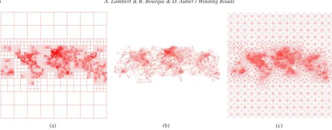
To obtain a multi-resolution grid graph, one can use a quad tree [FB74]. In a quad tree, the plane is decomposed in four parts until it contains at most one element. In figure1(a), one can see the grid graph generated on the 2000 air traffic network. Such an approach is efficient in terms of computa-tion time since its complexity is O(|V | · log(|V |)). However, on one hand it generates a large grid (37,395 nodes/69,102 edges for the 2000 AT network) and on the other hand, large cells promote horizontal and vertical paths. Voronoï di-agrams [Vor08] can also be used to generate the grid graph. In a voronoï diagram, cells are regions of the plane in which points of a cell are closer to the cell’s site (here original nodes) than to any other site. Figure1(b) shows the grid graph obtained with the Voronoï approach. Using classi-cal Voronoï diagram does not guarantee to avoid node edge overlap in case of non point size node. However that prob-lem can be easily addressed using a constrained Voronoï di-agram (taking node sizes into account). This method gener-ates a small grid graph (4,531 nodes/13,558 edges for the 2000 AT network) and can be computed in O(|V | · log(|V |)) time [For86]. However, it generates large cells for sparse re-gion. Due to our routing method, these large cells will cre-ate large detours. In this work, we propose a hybrid algo-rithm based on both quad trees and Voronoï diagrams. In our algorithm, the size of quad tree cells are parametrized to generate different levels of clutter reduction (see section5). Voronoï diagrams are then used to construct the final grid graph. Figure1(c)shows the grid graph obtained with this hybrid approach. Since the quad tree adds O(|V |) nodes, the O(|V | · log|V ]) time complexity is preserved. Therefore, the resulting grid graph is of reasonable size (10,146 nodes/ 30,315 edges on 2000 AT network).

3.2. Edge routing

The next step of our method consists of routing edges in the original graph onto the grid we obtained in the previ-ous step. We can use a shortest path algorithm directly to achieve this operation. Since the grid is planar, we obtain a polyline drawing of the graph. However, this method does not guarantee that edges follow the same path and thus it creates few bundles. To augment the bundling effect, we use the metaphor of roads and highways. The idea is to trans-form regular roads into larger ones if they are highly used. We reproduce this effect by first computing all the shortest paths between linked nodes on the original graph. Then, ac-cording to the number of shortest paths passing through an edge of our grid, we adjust the weights of the edge. Reduc-ing the weights of an edge is equivalent to transformReduc-ing it into a highway, since using that edge enables it to go faster from one point to another. We then compute a shortest path for each edge of the original graph. This weights

(5)

adjust-(a) (b) (c)

Figure 1: Grid graphs generated on the 2000 Air Traffic (AT) network with (a) a quad tree (37395 nodes/69102 edges), (b) a

Voronoi diagram (4531 nodes/13558 edges) and (c) the hybrid quad tree/Voronoï approach (10146 nodes/30315 edges).

com-plexity. To speed up the edge routing process we introduce in the next section several optimizations.

4. Implementation issues

A naive implementation of our approach can bundle graphs in a reasonable amount of time. In figure2, one can see that on the US migration graph [Hv09,CZQ∗₀₈_{] it takes}

75 seconds to bundle the graph with our approach. This ex-ecution time is faster than [Hv09] but significantly slower than [CZQ∗₀₈_{]. This benchmark was ran on an Intel(R)}

Core(TM)2 Extreme CPU Q9300 2.53GHz. To improve the efficiency of our method and make it usable on larger graphs, several optimizations must be done. In this section, we pro-pose optimizations that reduce the overall computation time. These optimizations consist of minimizing the number of shortest paths computed and taking advantage of modern multi-core architectures. These improvements do not change the output of the algorithm when compared to the straight-forward implementation. However, the execution time can be reduced by a factor of ten or more, depending on the num-ber of CPUs and the topology of the graph.

First optimization :The first optimization consists of re-ducing the time to compute the shortest paths. In our imple-mentation, we use Dijkstra’s algorithm [Dij71]. The weights of the edges are modified according to the paths we want to promote. Thus, we must use the weighted shortest path algorithm, and we can not use faster Euclidian graph short-est path methods [SV86]. If we use this straightforward ap-proach, we have to compute the shortest paths for each node of the original graph to each node of the grid. These op-erations can be done in O(|Vgraph|.|Egrid|.log|Vgrid|) time.

However, we only need the shortest path between each ad-jacent nodes of the original graph on the grid. With a slight modification to Dijkstra’s algorithm, we can stop the com-putation of paths when all candidates in the Dijkstra’s pri-ority queue are at a distance greater than all the neighbors of our source node. In figure2(a),2(b)and2(c)one can see that this modification significantly decreases running time. In figure2(c), one can see that the running time has been re-duced by a gain of factor 6.4. This call graph has been drawn with a force-directed algorithm [HJ04] which tries to lay out as close as possible connected nodes. Thus, this optimiza-tion allows us to restrict the exploraoptimiza-tion to a small part of the grid each time. This makes our algorithm efficient for graphs drawn with this kind of algorithm.

Second optimization :The second optimization aims to reduce the number of calls to the shortest path algorithm and also increases the efficiency of the previous one. After computing the shortest paths from one node to its neighbors, we don’t need to consider that node again during the com-putation. Minimizing the number of nodes to treat in order to consider each edge of the graph is the so called vertex cover problem [Hoc97]. Unfortunately this problem is NP-complete. However, it is possible to compute a minimal (but not optimal) vertex cover of a graph. Instead of using the original graph for computing the neighbors of a node in the first optimization, we construct a copy of that graph, called vertex cover graph, in which we delete a node after it has been treated. Deleting this node in the vertex cover graph re-duces the degree of its neighbors and thus it will reduce the set of nodes considered by the first optimization. In figure2, one can see that in all cases this improvement significantly decreases the running time of our technique.

Third optimization :The third optimization aims to re-duce the number of critical sections in the parallel imple-mentation of our algorithm and to create tasks of

(6)

equiva-A. Lambert & R. Bourqui & D. Auber / Winding Roads 5

(a) (b) (c)

Figure 2: Computation time of our method applied : (a) on the US migration graph used by [Hv09,CZQ∗₀₈_{] (}₁₇₁₅

vertices/9780 edges), (b) on the 2000 air traffic network (1525 vertices/16479) and (c) on the call graph (5741 vertices/11442

edges).

lent size for each thread. Our method needs to run a short-est paths algorithm for each vertex of our cover set. This approach can be parallelized by computing several short-est paths simultaneously. However, there are critical sections that one needs to address. For instance, the update of the number of shortest paths passing through a particular edge can be done by several threads in parallel. To remove these critical sections, we use a preprocessing step that creates sets of nodes which do not conflict with each other. We have tried the graph coloration heuristic of Welsh and Powell [WP67]. Our experimentation shows that it does not improve the run-ning time and it seems better to use critical sections instead. After several experiments, we found that the key is to cre-ate a local coloration before starting each parallel section. The algorithm maintains a list of nodes ordered according to the distances in the original layout to their neighborhood. Before each parallel section, we select the k (where k cor-responds to the number of threads) first nodes that are not connected. This operation prevents treating the same edge several times and generates a set of tasks with a more ho-mogeneous size. Indeed, the first optimization speeds up the computation of shortest paths if the neighbors are close to each other in the layout. Thus, if one treats in parallel nodes having close neighbors and far neighbors, the execution time of each thread can be significantly different. Using our or-dering, we ensure that we take a set of nodes in which the shortest path computation time is similar. In figure2, one can see that even if the scheduling adds extra computation time it allows us to speed up the overall running time.

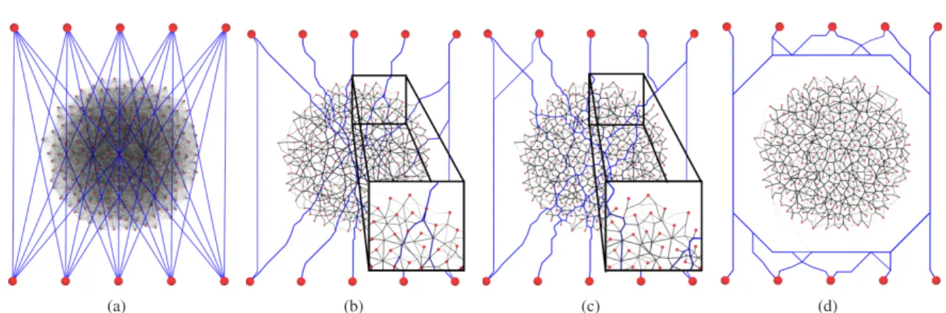
5. Level of Clutter Reduction

As described in previous sections, our method consists of routing the original edges on the grid graph using the well-known Dijkstra’s algorithm. Weighted shortest paths allow us to define different levels of clutter reduction by either adapting edge weights or avoiding a particular path. In fig-ure3, one can see the different levels of clutter reduction that we propose.

5.1. Edge-edge clutter reduction

The edge-edge clutter reduction we define corresponds to the one used in [CZQ∗₀₈_,_Hv09_{], i.e. only clutter due}

to edge crossings is reduced. In this case bundles of edges can overlap with nodes of the original graph. For instance, figure3.(b) shows the result obtained on the graph of fig-ure3.(a) using only edge-edge clutter reduction. One can see in the zoomed view that blue edges are routed through nodes of the network. To obtain this level of clutter reduction, one just has to consider each edge of the grid graph when routing the edges. In particular, a node-grid edges (i.e. edges linking original nodes to nodes of the grid graph) can be used when computing the shortest paths on the grid graph.

5.2. Node-edge clutter reduction

Edge-edge clutter reduction only allows us to reduce the clutter due to edge crossings. Still, one may want to unclutter the representation by reducing clutter due to node-edge over-laps. We can forbid routing node through the original graph. For instance, in figure3.(c), one can see that the blue edges are routed around nodes in the graph while these edges cross the nodes using edge-edge clutter reduction only. We obtain node-edge clutter removal by filtering out node-grid edges during Dijkstra’s algorithm. As these node-grid edges are not taken into account when computing the shortest paths, no original edge can be routed through a node of the original graph. Of course, path ending on original nodes are allowed.

5.3. Uncluttering highly dense zones

We can further improve clutter reduction by promoting paths to pass through sparse regions. For instance, in fig-ure3.(d), one can see that all blue edges have been routed

aroundthe dense subgraph (in the middle of figure3.(d)). Our method naturally produces this effect since paths pass-ing through dense regions are quite twisty. As the density in this part of the drawing is high, the corresponding region of the grid graph contains many cells. Therefore, the length of

(7)

(a) (b) (c) (d)

Figure 3: Different clutter reductions of a graph representation (a), using edge-edge clutter reduction method (b), avoiding

node-edge overlap (c) and uncluttering dense zones (d).

an edge routed through this part of the graph is longer than the Euclidian distance between its extremities. To augment this phenomena, dummy nodes are added around the original node when applying our quadtree method (see section3). We are able to unclutter even more dense regions by adapting the initial weights of the grid edges. Let l be the Euclidian dis-tance between two nodes in our grid (i.e. length of an edge). We compute the new weights using the following formula

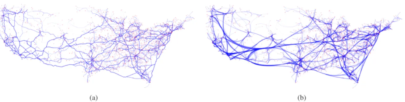
w(e) = length(e)α

, the α parameter can be used to increase or decrease the uncluttering of dense regions. An α less than one promotes path outside dense regions. In figure6.(b) one can see that edges going from bottom left to the bottom right corner are bundled on the south pole. It thus reduces clutter in the center of the map.

6. Interactive rendering of edge-bundled graphs 6.1. Smoothing the edges with curves

Once the bundling process has been performed on the graph, edges become polylines due to the routing phase which adds bends to them. With respect to the size of the graph and the grid used to compute the bundles, the number of edge bends can be quite high. When rendering the edge-bundled graph layout, these bends induce a “zigzag” effect on the edges making them hard to follow. In order to smooth edges, we offer the possibility of rendering them as curves in our visualization system using edge bends as curves control points. Several kinds of parametric curves are proposed in-cluding Bézier curves and cubic B-splines. Moreover, edges going to the same region of the graph and sharing succes-sive bends remain merged, giving a nicer impression of flows between different areas of the graph. However, even if this result is more visually appealing, one drawback of this tech-nique is that we re-introduce edge-node clutter in the draw-ing. Due to the high computational cost of rendering curves with a large number of control points , especially Bézier curves, we have developed a GPU-based implementation.

It allows us to draw a large number of curves defined by an arbitrary number of control points in real time, giving us the ability to smoothly interact with the graph drawing. As an example, a comparison between the polyline and Bézier curve rendering of the graph edges is shown in figure4.

6.2. Edge splatting

When edges have been merged into bundles, high-level edge patterns emerge on the graph drawing, giving a nice impression of flows between different regions of the graph. However, the information regarding the number of edges contained in a bundle is not easily seen in the drawing. In order to distinguish strong bundles from weak ones, we pro-pose an edge splatting technique to visually enhance them.

Our method is inspired from the GraphSplatting technique introduced by van Liere et al. in [vd03]. In this work, the au-thors represent a graph as a 2D continuous scalar field and calculate a splat field. GraphSplatting provides a way to vi-sualize continuous variations in the density of vertices which can help determine the structure of the underlying graph. Another work sharing similar features to this technique is the one by Chiricota et al. [CJM04]. They propose a technique to select points in a scatterplot representation by applying a Gaussian blur on the associated image. This blurring effect melts points forming a dense subregion of the scatterplot into a large patch that can help a user to identify and select clus-ters in the underlying data.

The following presents our rendering pipeline to visualize the density of edges that have been merged into bundles. It is based on a combination of common image processing and computer graphics technique and each stage entirely runs on the GPU. In a similar way than the GraphSplatting tech-nique, the idea is to compute a splat field encoding contin-uous variations in the density of merged edges. This splat field can then be displayed on screen in a various ways. We explored two solutions to visually encode bundles density.

(8)

A. Lambert & R. Bourqui & D. Auber / Winding Roads 7

(a) (b)

Figure 4: Comparison between two representations of an edge-bundled graph. In (a), edges are drawn as polylines while in (b)

they are drawn as Bézier curves. When edges are rendered as Bézier curves, their shapes are smooth and a nice impression of flows between different regions of the graph emerges from the drawing. However, edges can overlap nodes due to the lack of local control proper to Bézier curves.

The first one simply maps density values to colors based on a user-defined color scale. The second one preserves edges colors and uses a per-pixel shading technique mapping den-sity values to heights giving the impression than strong bun-dles appears higher than weak ones.

6.2.1. Computing and rendering the splat field

The first stage of our edge splatting rendering pipeline is to compute the number of edges crossing each pixel of the drawing. As in [Hv09], this operation can be done by performing an offscreen rendering of the graph edges in an accumulation buffer. Using the OpenGL graphics API, we can implement it with a render-to-texture technique using a

Frame Buffer Objectwith a single precision floating point texture attached to it. Then, we assign the same color to each edge and activate additive blending during the render-ing stage.

Next stage of the rendering pipeline is the splat field com-putation. The resulting texture of the previous stage is a field of discrete values encoding edges density per pixel. The goal of this stage is to transform it into a continuous scalar field. This process can be performed by convoluting the discrete density values field with a Gaussian kernel defined by a ra-dius r and a standard deviation σ. This operation can still be performed on the GPU by rendering to a texture and by writing an OpenGL fragment shader to perform the convolu-tion. A shader program allows to modify the default behav-ior of some processing units in the GPU rendering pipeline. A fragment shader aims to customize the pixel processing unit of the pipeline whose role is to calculate the colors of the pixels to display. In OpenGL, shader programs can be written using a C-like language called GLSL (the OpenGL

Shading Language). Shaders offer tangible benefits since they are well suited for parallel processing as most modern GPUs have multiple shader pipelines. Because a fragment shader allows reads of pixels from a texture stored in graph-ics memory, implementing the convolution of the discrete density values with a Gaussian kernel is an easy task. Our

Figure 5: Linear edge splatting generated with a Gaussian

kernel of radius 5 and standard deviation 3.

implementation takes advantage of the fact that a Gaussian filter is linearly separable. Therefore, we can divide the pro-cess into two passes [Smi97]. In this way, performances do not degrade as the radius of the kernel increases. The source code of this fragment shader is generated dynamically with respect to the kernel radius requested by the user. The stan-dard deviation of the Gaussian kernel can also be modified dynamically. The larger the kernel radius and standard devi-ation, the more the splat field is smoothed.

In order to visualize the computed splat field, a gradient-based rendering is performed, mapping the splatting value associated to each pixel to a user-defined color scale. To achieve this task, the minimum and maximum value of the splat field are determined with a GPU texture reduce op-eration [KW03]. A quadrilateral with the same size as the splat field texture is then drawn to the screen and pixel col-oring is performed by a dedicated fragment shader, mapping splatting values to the user-defined gradient. The result of the edge splatting technique on the US migration graph is presented in figure5.

6.2.2. Enhancing the splatting with shading

As a way of improving the splat field representation, we propose an extra rendering stage based on a bump mapping

(9)

technique. Bump mapping is a computer graphics technique introduced by Blinn [Bli78] allowing a rendered surface to appear more realistic without modifying geometry. It adds a per-pixel shading that makes the surface appears bumpy, by changing the surface normals. The colors and brightnesses of the pixels are then altered with respect to these normals using a lighting algorithm. The modified normal for each pixel are stored in a texture called a normal map. RGB com-ponents of the pixels colors store the X, Y and Z values of the normal vectors. This normal map is generated from a

heightmap, another texture storing the height values for each pixel of the surface. Bump mapping is classified in the per-pixel displacement mapping methods. An exhaustive survey of these displacement mapping algorithms is presented by Szirmay-Kalos et al. [SKU08].

Recently, Willems et al. proposed a geographical visual-ization of vessel movements [Wvv09] where they used shad-ing to highlight significant maritime areas, like highways or anchoring zones. Their visualization is based on density fields that are derived from the convolution of dynamic ves-sel positions with a kernel. In our case, if we map splat-ting values to heights, we can use bump mapping to enhance edge-bundled graph visualizations. Bundles with high den-sity edges will appear higher than others with this rendering technique and will visually emerge from the layout. In order to achieve this task, we first need to generate a heightmap from the computed splat field. This map can be generated by mapping the splatting values to a black to white color scale : black representing minimum height and white representing maximum height. Then, we can generate the associated nor-mal map by obtaining the heightmap gradient using for in-stance the Sobel or Prewitt filter [GW06]. This operation can be performed on the GPU with a fragment shader. This pro-gram compute for each pixel the heightmap derivatives in horizontal and vertical directions using the gradient operator and construct the associated normal from these.

Once the normal map associated with the splat field has been generated, bump mapped rendering can be performed. The bump mapped is generated by a dedicated shader

pro-gram reading the modified normals from the normal map texture and performing a per-pixel illumination using Blinn-Phong [Bli77]. The final colors of the pixels are computed from the lighting properties and another texture called the

diffuse map. In our case, the diffuse map can correspond to the splat field color mapping or the original edge colors. To perform a global illumination, the light is set to be direc-tional with each light ray parallel to the Z-axis. Our visual-ization system then lets the user configure the ambient, dif-fuse and specular color of the light source. Results of this rendering technique are presented in figure6.

6.2.3. Rendering performances

In table1, we introduce an estimation of the running time for the edge splatting rendering pipeline. The benchmarks

have been ran on two different edge-bundled graphs con-taining at least ten thousands edges. The table provides esti-mation for the whole pipeline traversal but also for its three main stages : density map generation, splat field computa-tion (includes Gaussian convolucomputa-tion and GPU reduccomputa-tion) and bump mapping rendering (includes diffuse map, heightmap and normal map generation). The introduced performances have been measured by executing one hundred times the edge splatting pipeline and by computing the average ren-dering times. As shown by the results, the most expensive stage is the density map generation. During that process, the rendering of the whole graph edges set is required. Bundled edges can have a high number of bends so the number of vertices sent to the GPU is much larger when compared to straight line rendering. Obviously, the Bézier curve render-ing is more expensive than the polyline one due to the high computational cost of curves generation. The two remaining stages of the rendering pipeline can be executed in real time with respect to the measured framerates. Eventually, perfor-mances are acceptable with respect to the number of edges bends. For instance, the whole pipeline traversal for the US migration graph, which contains ten thousands edges with a large number of bends, takes around 0.1 seconds for the polyline rendering and around 0.5 seconds when rendering edges as Bézier curves.

graph US Migration Air Traffic #nodes / #edges 1715 / 9778 1533 / 16525 #bends per edges

(#control points for curves)

from 1 to 213 mean : 30

from 0 to 203 mean : 29 Whole edge splatting

rendering pipeline (shape : polyline) 0.103 s. (9.7 FPS) 0.17 s. (5.74 FPS) Whole edge splatting

rendering pipeline (shape : Bézier) 0.52 s. (1.92 FPS) 0.57 s. (1.74 FPS) Density map generation

(shape : polyline)

0.09 s. (11.1 FPS)

0.15 s. (6.15 FPS) Density map generation

(shape : Bézier)

0.51 s. (1.96 FPS)

0.56 s. (1.78 FPS) Splat field computation _{(85 FPS)}0.012 s. _{(94.8 FPS)}0.011 s. Bump mapping rendering _{(2250 FPS)}0.00044 s. _{(2185 FPS)}0.00046 s.

Table 1: Performances of edge splatting rendering for

dif-ferent edge-bundled graphs. Rendering is performed in a viewport whose size in pixels is 800 x 800. Edge splatting is performed with a Gaussian kernel of radius 3. The nor-mal map needed for bump mapping is generated with a 5 x 5 Prewitt Filter. The CPU used to perform these tests is an Intel(R) Core(TM)2 Extreme CPU X9100 @ 3.06GHz and the graphic card is a NVidia Quadro FX 1700M.

7. Conclusion

In this paper, we have presented a novel and intuitive tech-nique to route edges into bundles. This techtech-nique reduces the clutter of the representation and also emphasizes high-level edge patterns. Optimizations of our technique allow us to outperform the execution times of existing methods and

(10)

A. Lambert & R. Bourqui & D. Auber / Winding Roads 9

(a)

(b)

Figure 6: Illustrations of the bump mapping based rendering of edge splatting with the edge-bundled representations of the

US migration graph and 2000 AT network. Strong bundles appears higher than other ones with this technique making them visually emerge from the graph drawing. For the US migration graph, heights are linearly mapped to the splat field and the diffuse map used for the bump mapping rendering corresponds to the splat field linear color mapping. For the AT graph, heights are logarithmically mapped to the splat field and the original edges colors are used as diffuse map.

scale to larger graphs. In addition to edge-edge clutter reduc-tion, our method can guarantee that no node-edge overlaps occurred in the drawing. Moreover, by promoting long grid edges, we can further reduce edge cluttering in highly dense regions and preferably bundle edges in sparse ones.

Using curves when rendering edges facilitate informa-tion discovery as it eases the following of bundles. We ex-tend the GraphSplatting technique to edge splatting in or-der to depict bundles densities. Finally, a bump mapping technique enhances the edge splatting and also makes it possible to preserve the color encoding of the edges. Our GPU-implementation allows fast enough rendering to sup-port smooth interaction.

An interesting direction for future work is to explore dif-ferent methods to build the grid graph such as constrained Delaunay triangulations. More specifically, a grid support-ing non-uniform node sizes would allow bundles to avoid

regions of the image in order to display nodes labels, cap-tions, color scales or any other information. We also plan to adapt our method to the sphere, to surfaces having other topologies, or even 3D space.

Improving the curves smoothing technique also remains future work. On one hand, we want to constrain our curves to avoid nodes. On the other hand, we want to speed up the rendering by minimizing the number of bends, while also guarantying that no node-edge overlap is created.

References

[AMA07] ARCHAMBAULT D., MUNZNER T., AUBER D. :

Grouse : Feature-Based and Steerable Graph Hierarchy Explo-ration. In Eurographics/ IEEE-VGTC Symposium on

Visualiza-tion(Norrköping, Sweden, 2007), Museth K., Möller T., Ynner-man A., (Eds.), Eurographics Association, pp. 67–74.1 [Aub03] AUBERD. : Tulip : A huge graph visualisation

(11)

Mathematics and Visualization. Springer-Verlag, 2003, pp. 105– 126.2

[AvK06] ABELLO J., VAN HAM F., KRISHNAN N. :

ASK-GraphView : A Large Graph Visualisation System. IEEE

Trans-actions on Visualization and Computer Graphics 12, 5 (2006), 669–676.1

[Bli77] BLINNJ. F. : Models of light reflection for computer synthesized pictures. In SIGGRAPH ’77 : Proceedings of the 4th

annual conference on Computer graphics and interactive tech-niques(New York, NY, USA, 1977), ACM, pp. 192–198.8 [Bli78] BLINNJ. F. : Simulation of wrinkled surfaces. In

SIG-GRAPH ’78 : Proceedings of the 5th annual conference on Com-puter graphics and interactive techniques(New York, NY, USA, 1978), ACM, pp. 286–292.8

[CJM04] CHIRICOTAY., JOURDANF., MELANCONG. : Metric-based network exploration and multiscale scatterplot. In Proc.

of IEEE Information Visualization Symposium(Washington, DC, USA, 2004), IEEE Computer Society, pp. 135–142.6

[CZQ∗_08] _C_UI_{W., Z}_HOU _{H., Q}_U _{H., W}_ONG_{P. C., L}_I _{X. :}

Geometry-based edge clustering for graph visualization. IEEE

Transactions on Visualization and Computer Graphics 14, 6 (2008), 1277–1284.2,3,4,5

[DEGM03] DICKERSONM., EPPSTEIND., GOODRICHM. T., MENGJ. Y. : Confluent Drawings : Visualizing Non-planar Di-agrams in a Planar Way. In Proc. Graph Drawing 2003 (GD’03) (2003), pp. 1–12.2

[DGKN98] DOBKIN D., GANSNER E., KOUTSOFIOS E.,

NORTH S. : Implementing a general-purpose edge router. In

Proc. Graph Drawing 1997 (GD’97)(1998), pp. 262–271.2 [Dij71] DIJKSTRAE. W. : A short introduction to the art of

pro-gramming. Technische Hogeschool Eindhoven, 1971.4 [DN10] DWYERT., NACHMANSONL. : Fast Edge-Routing for

Large Graphs. In Proc. Graph Drawing 2009 (GD’09) (2010), p. To appear.2

[ED07] ELLISG., DIXA. : A taxonomy of clutter reduction for information visualisation. IEEE Transactions on Visualization

and Computer Graphics 13, 6 (2007), 1216–1223.2

[FB74] FINKEL R. A., BENTLEY J. L. : Quad trees a data structure for retrieval on composite keys. Acta Informatica 4, 1 (March 1974), 1–9.3

[FLM94] FRICKA., LUDWIGA., MEHLDAUH. : A Fast Adap-tive Layout Algorithm for Undirected Graphs. In Proc. Graph

Drawing 1994 (GD’94)(1994), pp. 388–403.1

[For86] FORTUNES. : A sweepline algorithm for Voronoi dia-grams. In SCG ’86 : Proc. of the second annual symposium on

Computational geometry(1986), pp. 313–322.3

[GK06] GANSNERE. R., KORENY. : Improved circular layouts. In Proc. Graph Drawing 2006 (GD’06) (2006), pp. 386–398.2 [GW06] GONZALEZR. C., WOODSR. E. : Digital Image

Pro-cessing (3rd Edition). Prentice-Hall, Inc., Upper Saddle River, NJ, USA, 2006, ch. 10, pp. 707–710.8

[HJ04] HACHULS., JÜNGERM. : Drawing Large Graphs with a Potential-Field-Based Multilevel Algorithm. In Proc. Graph

Drawing 2004 (GD’04)(2004), pp. 285–295.1,4

[Hoc97] HOCHBAUMD. S. : Approximating covering and pack-ing problems : set cover, vertex cover, independent set, and re-lated problems. 94–143.4

[Hol06] HOLTEND. : Hierachical Edge Bundles : Visualization of Adjacency Relations in Hierarchical Data. IEEE Transactions

on Visualization and Computer Graphics 12, 5 (2006), 805–812. 2,3

[Hv09] HOLTEN D., VAN WIJK J. J. : Force-directed edge bundling for graph visualization. In 11th

Eurographics/IEEE-VGTC Symposium on Visualization (Computer Graphics Forum ; Proceedings of EuroVis 2009)(2009), vol. 31, pp. 983–990.2,3, 4,5,7

[KW03] KRÜGERJ., WESTERMANNR. : Linear algebra opera-tors for GPU implementation of numerical algorithms. In

SIG-GRAPH ’03 : ACM SIGSIG-GRAPH 2003 Papers(New York, NY, USA, 2003), ACM, pp. 908–916.7

[PXY∗_05] _P_HAN_{D., X}_IAO_{L., Y}_EH_{R., H}_ANRAHAN_{P., W}_INO -GRADT. : Flow map layout. In Proc. of IEEE Information

Visualization Symposium(Washington, DC, USA, 2005), IEEE Computer Society, pp. 219–224.2

[SKU08] SZIRMAY-KALOSL., UMENHOFFERT. : Displacement mapping on the GPU - State of the Art. Computer Graphics

Forum 27, 1 (2008).8

[Smi97] SMITH S. W. : The scientist and engineer’s guide to

digital signal processing. California Technical Publishing, San Diego, CA, USA, 1997, ch. 24, pp. 404–407.7

[SV86] SEDGEWICKR., VITTERJ. S. : Shortest paths in eu-clidean graphs. Algorithmica 1 (nov 1986), 31–48.4

[vd03] VANLIERER.,DELEEUWW. : GraphSplatting : izing graphs as continuous fields. IEEE Transactions on

Visual-ization and Computer Graphics 9, 2 (2003), 206–212.6 [Vor08] VORONOIG. : Nouveles applications des paramètres

continus à la théorie de formas quadratiques. J Reine Angew

Math 134(1908), 198–287.3

[vv04] VANHAMF.,VANWIJKJ. J. : Interactive Visualization of Small World Graphs. In Proc. of IEEE Information

Visualiza-tion Symposium(Washington, DC, USA, 2004), IEEE Computer Society, pp. 199–206.1

[WC05] WONGN., CARPENDALES. : Using Edge Plucking for Interactive Graph Exploration. In Proc. of IEEE Information

Vi-sualization Symposium, Poster Compendium(Washington, DC, USA, 2005), IEEE Computer Society, pp. 51–52.2

[WCG03] WONGN., CARPENDALES., GREENBERGS. : Edge-Lens : An Interactive Method for Managing Edge Congestion in Graphs. In Proc. of IEEE Information Visualization Symposium (Washington, DC, USA, 2003), IEEE Computer Society, pp. 51– 58.2

[WMS06] WYBROW M., MARRIOTT K., STUCKEY P. :

In-cremental connector routing. In Proc. Graph Drawing 2005

(GD’05)(2006), pp. 446–457.2

[WP67] WELSHD. J., POWELLM. B. : An upper bound to the chromaticnumber of a graph and its application to timetabling problems. The Computer journal 10 (1967), 85–86.5

[Wvv09] WILLEMS N., VAN DE WETERING H., VAN WIJK

J. J. : Visualization of vessel movements. In 11th

Eurographics/IEEE-VGTC Symposium on Visualization (Com-puter Graphics Forum ; Proceedings of EuroVis 2009) (2009), vol. 31, pp. 959–966.8

[ZYC∗_08] _Z_HOU_{H., Y}_UAN_{X., C}_UI_{W., Q}_U_{H., C}_HEN_{B. :}

Energy-based hierarchical edge clustering of graphs. In

Visu-alization Symposium, 2008. PacificVIS ’08. IEEE Pacific(2008), pp. 55–61.3