HAL Id: hal-00880980
https://hal.archives-ouvertes.fr/hal-00880980
Submitted on 8 Nov 2013
HAL is a multi-disciplinary open access
archive for the deposit and dissemination of
sci-entific research documents, whether they are
pub-lished or not. The documents may come from
teaching and research institutions in France or
abroad, or from public or private research centers.
L’archive ouverte pluridisciplinaire HAL, est
destinée au dépôt et à la diffusion de documents
scientifiques de niveau recherche, publiés ou non,
émanant des établissements d’enseignement et de
recherche français ou étrangers, des laboratoires
publics ou privés.
classification with sparse SVM
Devis Tuia, Michele Volpi, Mauro Dalla Mura, Alain Rakotomamonjy, Rémi
Flamary
To cite this version:
Devis Tuia, Michele Volpi, Mauro Dalla Mura, Alain Rakotomamonjy, Rémi Flamary. Automatic
Feature Learning for spatio-spectral image classification with sparse SVM. IEEE Transactions on
Geoscience and Remote Sensing, Institute of Electrical and Electronics Engineers, 2014, 52 (10),
pp.6062-6074. �10.1109/TGRS.2013.2294724�. �hal-00880980�
Automatic feature learning for spatio-spectral image
classification with sparse SVM
Devis Tuia, Member, IEEE, Michele Volpi, Student Member, IEEE,
Mauro Dalla Mura, Member, IEEE, Alain Rakotomamonjy, R´emi Flamary
Abstract—Including spatial information is a key step for suc-cessful remote sensing image classification. Especially when deal-ing with high spatial resolution (in both multi- and hyperspectral data), if local variability is strongly reduced by spatial filtering, the classification performance results are boosted. In this paper we consider the triple objective of designing a spatial/spectral classifier which is compact (uses as few features as possible), discriminative (enhance class separation) and robust (works well in small sample situations). We achieve this triple objective by discovering the relevant features in the (possibly infinite) space of spatial filters by optimizing a margin maximization criterion. Instead of imposing a filterbank with pre-defined filter types and parameters, we let the model figure out which set of filters is optimal for class separation. To do so, we randomly generate spatial filterbanks and use an active set criterion to rank the candidate features according to their benefits to margin maximization (and thus to generalization) if added to the model. Experiments on multispectral VHR and hyperspectral VHR data show that the proposed algorithm, which is sparse and linear, finds discriminative features and achieve at least the same performances as models using a large filterbank defined in advance by prior knowledge.
Index Terms—Feature selection, Classification, Hyperspectral, Very high resolution, Mathematical morphology, Texture, At-tribute profiles
I. INTRODUCTION
R
ECENT advances in optical remote sensing opened new highways for spatial analysis and geographical applica-tions. Urban planning, crops monitoring, disaster management: all these applications are nowadays aided by the use of satellite images that provide a large scale and non-intrusive observation of the surface of the Earth.Two types of new generation sensors have attracted great attention from the research community: very high spatial res-olution (VHR) and hyperspectral sensors (HS). VHR images
Manuscript received XXXX;
This work has been partly supported by the Swiss National Science Foundation (grants PZ00P2-136827 and 200020-144135)) and by the French ANR (09-EMER-001, 12-BS02-004 and 12-BS03-003).
DT is with the Laboratoire des Syst`emes d’Information G´eographique (LaSIG), Ecole Polytechnique F´ed´erale de Lausanne (EPFL), Switzerland. [email protected], http://devis.tuia.googlepages.com, Phone: +41-216935785, Fax : +41-216935790.
MV is with the Centre for Research on Terrestrial Environment,
Universit´e de Lausanne (UNIL), Switzerland. [email protected],
http://www.kernelcd.org. Phone: +41-216923543, Fax : +41-216924405. MDM is with Grenoble Images Speech Signals and Automatics Lab (GIPSA-lab), Grenoble Institute of Technology (Grenoble INP), France. [email protected], Phone: +33 (0)4 76 82 64 11.
AR is with LITIS EA 4108, Universit´e de Rouen, France. [email protected]
RF is with Lagrange laroratory, Universit´e de Nice Sophia-Antipolis, CNRS, Observatoire de la Cˆote d’Azur, F-06304 Nice, France. [email protected]
have the advantage of providing pixels with meter or even sub-meter geometrical resolution (ground sample distance), and thus permit to observe fine objects in urban environments, such as details on buildings or cars, with enhanced precision in their spatial description [1]–[5]. Typically, VHR images are characterized by a limited spectral resolution since they can only acquire few spectral channels (a single one for panchromatic images, and less than ten for multispectral ones). On the contrary, HS images are capable of a finer sampling of the continuous electromagnetic spectrum, sensing the surveyed surface in up to hundreds of narrow contiguous spectral ranges (typically, each band has a range of about 5-20 nm). This type of imagery can be very useful for agriculture [6], [7] or forestry [8], [9], since it allows to discriminate types of vege-tation and it inspects their conditions by fully exploiting subtle differences in their spectral reflectance [10]–[12]. However, the enhanced spectral resolution of HS imagery does not generally allow a very high spatial resolution: for satellite HS, resolution is typically of the order of decameters. On the contrary, airborne new generation sensors, such as APEX [13], or more recent solutions based on unmanned aerial vehicles [14], allow nowadays to obtain VHR HS imagery, thus combining the advantages (and drawbacks) of both types of sensors.
Despite the potential of new generation remote sensing, the complexity of imagery of high resolution (either spatial or spectral) greatly limits their complete exploitation by the application communities in a daily use. Considering a classi-fication task, on the one hand VHR images tend to increase the intraclass spectral variance, as each type of landcover is contaminated by the signature of the objects composing it. For instance, antennas or flowers on a roof can mix the signature of the tiles composing the roof with the one of metal or vegetation. Furthermore, even if these objects are correctly classified thanks to the high spatial resolution, their presence makes the extraction of their semantic class (e.g., the whole rooftop) more difficult.
On the other hand, HS images are confronted to problems in the efficiency of data handling due to computational and memory issues related to the large number of bands acquired. Moreover, high dimensionality makes the modeling of the class distributions more difficult to achieve, typically resulting in degenerate solutions given by small sample scenarios. For all these reasons, classifiers exploiting spatial information extracted from hyperspectral data, but also applying dimension reduction, tend to achieve better results than purely spectral classifier applied on high dimensional feature spaces [10], [15].
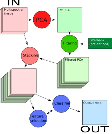
PCA
Stacking Classifier Feature selection Filtering 1st PCA Output map Filterbank (pre-defined) Multispectral image Filtered PCAIN
OUT
Fig. 1. Standard flowchart for spatio-spectral classification.
These two problems have been tackled by two contradictory, but related solutions: the first problem by the inclusion of spatial information [2], [15]–[17], i.e. the augmentation of the feature space by adding some spatial (e.g. contextual) features enhancing the discrimination between spectrally sim-ilar classes. Contextual features typically provide information about the distribution of greylevels in a spatial neighborhood of the pixel. There is a plethora of spatial features that have been considered in the literature, the main being tex-tural [3], [4], [18]–[20], morphological [16], [17], [21]–[26], Gabor [27], [28], wavelets [29]–[31] and shape indexes [32], [33]. The second issue related to the high dimensionality of the input data has mainly been tackled by feature selection [?], [2], [34], [35] or extraction [?], [16], [36]–[38] techniques, i.e. the reduction of the feature space to a subspace containing only the features which are considered to be the most important to solve the problem.
When dealing with VHR HS images, the two aspects appear simultaneously. In this case, the common practice is to apply a predefined filterbank using prior knowledge on global, low frequency features (for example a panchromatic image [4], the first PCAs [16] or other features extracted with supervised or unsupervised approaches [39]). Subsequently, the enriched input space (the spatial features only [2], [4], [16] or a combination of the spatial and spectral features [24], [40], [41]) is entered into a classifier, often applying an additional feature selection/extraction phase to reduce the dimensionality of the enriched space [4], [24]. Figure 1 summarizes this standard procedure.
However, this procedure has many drawbacks: first, the
filterbank is predefined and thus scale and image dependent. As a consequence, the creation of such a specific set requires expert knowledge from the user. Second, in the case of HS images, the first feature extraction step is compulsory and also imposed, as it is not possible to extract all the contextual features from each spectral band. The choice of the feature extraction technique directly influences classifier accuracy, since the retained features or the criteria they optimize might be suboptimal for class discrimination. Lastly, the optimization of a classifier with integrated feature selection, in particular when dealing with a large filterbanks, is often computationally very costly.
In this paper, we consider these drawbacks in detail and propose a joint solution: we let the model discover the good features by itself. A desirable model is compact (contains as few features as possible), discriminative (the features enhance class separation) and robust (works well in situations charac-terized by the availability of few labeled samples). Achieving these three objectives simultaneously is extremely challenging, especially since the space of possible spatial filters and feature extraction methods is potentially infinite. We tackle the first and last objective by proposing the use of a sparse ℓ1 linear
support vector machine [43], which naturally performs feature selection without recurring to specific heuristics. Contrary to standard support vector machines, which minimize theℓ2norm
of the model weights, the proposed classifier minimizes theℓ1
norm, which forces most of the weights of the features to be zero and thus performs selection of the relevant features among a pre-defined set. Then, by extending the optimality conditions of the sparse ℓ1 norm support vector machine, we are able
to provide a sound theoretical condition to asses whether a novel feature would improve the model after inclusion. This permits the exploration of a potentially infinite number of features. The proposed algorithm bears resemblance to the online feature selection algorithm described in [44]. While both approaches alternate between the optimization of a model given a finite set of features followed by the selection of a novel feature, [44] uses an heuristic for assessing the goodness of the new feature. This strategy has also been used in remote sensing classification [45]. In this contribution, they tend to separate the feature selection step and classifier learning step by proposing several criteria for feature selection (hill climbing, best fit, grafting), whereas we focus on a global regularized empirical risk minimization problem leading to a unique criterion (optimal w.r.t the risk). Moreover their results suggest that the use of ℓ1 regularization leads to the
best feature selection, which emphasize the interest of our approach. Another related paper is [46], where the authors use genetic algorithms to select features from a possibly infinite bag of randomly generated features. In this case, the feature selection phase is prior to classification.
The second problem is the most complex and is the main contribution of this article. We do not want the model only to be sparse on the current set of features, but also to automat-ically discover a relevant set of featureswithout imposing it in advance.By relevant, we mean a set of features enhancing class separation is a margin-maximization sense. To discover the relevant features, we explore the possibly infinite space
of spatial filters, and assess whether one of the features considered would improve class separation if added to the model. The relevant features are discovered within a random subset of the infinite set of possible ones, queried iteratively: the size and richness of such set defines the portion of the filter
space that has been screened. To avoid trial-and-error or
re-cursive strategies involving model re-training for each feature
assessment, we propose to use a large margin-based fitness
function and an active set algorithm proposed by the authors in [47]. Since we do not make assumptions on which band is to be filtered, the type of features to be generated, or their parameters, we explore the high dimensional (and continuous, thus possibly infinite) space of features and retrieve the optimal set of filters for classification. Unlike recursive strategies, we re-train the SVM model only when a new feature has been highlighted as relevant and has been added to the current input space.
Finally, it is worth underlining that the feature optimization is performed separately for each class, as the relevant spatial variables might be different for classes with varying spatial characteristics (e.g., roads can be better enhanced by spatially anisotropic filters whereas crops by textural ones).
Experiments conducted on a multi-spectral VHR and VHR HS images confirm these hypothesis and allow one to identify and qualify the important filters to efficiently classify the scenes. The proposed method constructs class-specific filter-banks that maximize the margin with respect to the other classes, in a one-against-all discrimination setting.
A significant improvement in accuracy with respect to ℓ2
SVM with predefined sets of features was not the principal aim. Indeed, the main advantage of the proposed approach is the ability to select automatically from an extremely large set of potential features, hence alleviating the work of the user. We believe that it is easier for a non-specialist to define a sensible interval of values instead of a fixed sampling for feature extraction parameters. The conjunction of a sparse SVM with this automatic feature selector provides a reduced amount of filters that maximizes class separation, which is thus desirable from both the prediction and model compactness perspectives. We also show that the selected features can be efficiently re-used in a traditional ℓ2 SVM, thus leading to
additional boosts in performance . Finally, the discovery of the compact discriminative set of filters from the large input space is also beneficial in scenarios dealing with a limited number of training samples, since the amount of sparsity can be controlled.
The reminder of the paper is as follows: Section II presents the proposed methodology and the active set algorithm. Sec-tion III presents the VHR and HS data used in the experi-ments, that are detailed and discussed in Section IV. Finally, Section V concludes the paper.
II. LEARNING WITH INFINITELY MANY FEATURES Consider a set of n training examples {xi, yi}ni=1 where
xi∈ Rbcorresponds to the vector characterizing a pixel in the image with b bands and yi∈ {−1, 1} to its label. We define
a θ-parametrized function φθ(·) that maps a given pixel into
some feature space (the output of a filter or feature extraction).
Let F be the set of all possible finite subset of features andϕ an element of F composed of d features {φθj}
d i=1, in
the following called active set. For a given x, we denote as Φϕ(x) the vector of Rdwhosej-th component is φθj(x). Note
that the vectorΦϕ(x) only involves a finite number of feature
mapsd with associated parameters {θj}dj=1. We also suppose
in the sequel that P
iφθj(xi)
2
= 1, ∀θj which means that
the vector resulting from the application of a feature map to all the pixels is unit-norm. This normalization is necessary in order to compare fairly features with different range of values. In this framework, we are looking for a decision function f (·) of the form f (x) = d X j=1 wjφθj(x) = w TΦ ϕ(x) (1)
with w = [w1, . . . , wd]T the vector of all weights in the
decision function.
We propose to learn both the best finite set of feature maps ϕ (i.e., φs and θs) and the f (·) function by jointly optimizing the following problem:
min ϕ∈F minw n X i=1 H(yi, wTΦϕ(xi)) + λkwk1 (2)
whereH(y, f (x)) = max(0, 1 − yf(x))2
is the squared hinge loss and λ is a regularization parameter. The squared hinge loss is selected for optimization reasons. Indeed, since it is differentiable, it allows us to use efficient gradient descent
optimization in the primal as discussed in [?].This is a bilevel
optimization problem but for a fixed ϕ, optimizing the inner problem boils down to aℓ1 regularized linear SVM.
The optimality conditions of the problem (2) are [43]: rθj + λ sign(wi) = 0 ∀j wj 6= 0 (3) |rθj| ≤ λ ∀j wj = 0 (4) |rθ| ≤ λ ∀φθ6∈ ϕ (5) with rθ= −2 X i φθ(xi) max(0, 1 − yiwTΦϕ(xi)) (6) the scalar product between feature φθ(·) and the hinge loss
error, which can be interpreted as the alignment between the current prediction error and the feature under consideration. Optimality conditions (3) and (4) are the usual conditions for aℓ1regularized SVM, i.e. for the inner problem of (2), while
condition (5) is the optimality condition related to features that are not included in the active setϕ. Interestingly, this last condition shows that at optimality, if a feature is not included in the active set, then it has the same optimality condition as if it were included in the active with a0 weight.
These optimality conditions suggest the use of an active set algorithm that solves iteratively the inner problem, restricted to the features in the current active setϕ. At each iteration, if a feature not in the active set violates optimality constraint (5), it is added to the active set of the next iteration, leading to a decrease of the cost after re-optimization of the inner problem.
Algorithm 1 Active set algorithm Inputs
- Initial active set ϕ 1: repeat
2: Solve aℓ1 SVM with current active setϕ
3: Generate a new feature bank{φθj}
p j=1∈ ϕ/ 4: Computerθj as in (6)∀j = 1 . . . p 5: Find featureφ∗ θj maximizing |rθj| 6: If|rθ∗ j| > λ + ǫ, then ϕ = φ ∗ θj ∪ ϕ
7: until stopping criterion is met
In addition, if theith feature in the active set has a zero weight after re-optimization (i.e., wi = 0) it can be removed from
the active set in order to keep small the size of the inner problem. Note that Equation (6) demonstrates the necessity of normalized features. Without unit-norm normalization, feature will be selected by their norm and not by their alignment with the classification residuals.
With continuously parametrized filters, the number of pos-sible features could be infinite, so a comprehensive test of the candidate features is intractable. In this situation, [48] proposed to randomly sample a finite number of features and add to the active set the one violating the most constraint (5). Furthermore, in order to ensure convergence in a finite number of iteration, we choose to use anǫ−approximate condition for updating the active set. A featureφθ is added to the active set
only if |rθ| > λ + ǫ. The resulting approach is provided in
Algorithm 1.
Note that the algorithm is designed to handle large scale datasets. Indeed checking the optimality conditions and se-lecting a new feature has complexity O(n) and solving the inner problem is performed only on a small number of features di using an accelerated gradient algorithm combined with
a warm-starting scheme (see [48]). Note that the active set strategy allows to solve several small scale problems with a
number of features di ≪ d. The iteration complexity of the
inner problem solver at iteration i of algorithm 1 line 2 is
O(ndi). For comparison, using a classical linear SVM on d
features requires the computation of aO(nd) gradient at each
iteration, and a O(d3
) matrix inversion for a second order
solver such as [?]. Moreover, a warm starting scheme is used
at each iteration in the incremental algorithm. This means that a reasonable solution is provided to the ℓ1 SVM solver as
starting point, thus providing faster convergence with respect to a random or zero initialization.
III. DATA AND SETUP A. Datasets
Experiments have been carried out on two classification tasks, the former considering a VHR urban problem and the latter an agricultural scene sensed with a HS sensor.
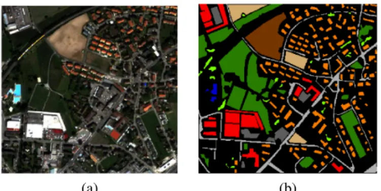
a) Br ¨uttisellen 2002 (QuickBird sensor, VHR): the first image is a 4-bands optical image of a residential neighborhood of the city of Zurich (Switzerland), named Br¨uttisellen, acquired in 2002 (Fig. 2). The image has a size of 329 × 347 pixels, and a geometrical resolution
(a) (b)
Fig. 2. Zurich Br¨uttisellen QuickBird data. (a) RGB composition and (b)
ground truth. Color references are in Tab. I (unlabeled samples are in black). TABLE I
LEGEND AND NUMBER OF LABELED SAMPLES AVAILABLE FOR THE
BRUTTISELLEN¨ 2002DATA
ID Color Class name No samples
1 Residential 6746 2 Commercial 5277 3 Meadows 14225 4 Harvested vegetation 2523 5 Bare soil 3822 6 Roads 6158 7 Pools 283 8 Parkings 1749 9 Trees 2615
of 2.4m. Nine classes of interest have been highlighted by photointerpretation and 40, 762 pixels are available (see Tab I). Spatial context is necessary to discriminate spectrally similar classes such as ‘trees’ – ‘meadows’ and ‘roads’ – ‘parking lots’.
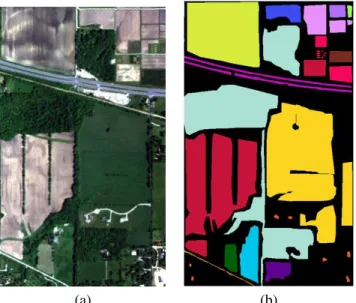
b) Indian Pines 2010 (ProSpecTIR spectrometer, VHR HS): the ProSpecTIR system acquired multiple flightlines near Purdue University, Indiana, on May 24-25, 2010 (Fig. 3). The image subset analyzed in this study con-tains 445×750 pixels at 2m spatial resolution, with 360 spectral bands of 5nm width. Sixteen land cover classes were identified by field surveys, which included fields of different crop residue covers, vegetated areas, and man-made structures. Many classes have regular geometry associated with fields, while others are related with roads and isolated man-made structures. Table II shows class labels and number of training samples per class. B. Experimental setup
In the experiments, we tested different initial setups, to assess stability of the method with respect to initial conditions. In all cases, we report average results over five independent starting training sets. We run the active set algorithm (AS) for 200 iterations for each class, thus discovering the discriminant features for each class separately. This means that we extract at most200 features per class. The algorithm stops according to two criteria: i) either the 200 iterations are met or ii) 40 filter generations have not provided a single feature violating the constraint of Eq. (5) byǫ.
a) Br ¨uttisellen 2002: we extracted 5% of the available training samples randomly and used them to optimize the
(a) (b)
Fig. 3. Indian Pines 2010 SpecTIR data.(a) RGB composition and (b) ground truth. Color references are in Tab. II (unlabeled samples are in black).
TABLE II
LEGEND AND NUMBER OF LABELED SAMPLES AVAILABLE FOR THE
INDIANPINES2010DATA
ID Color Class name No. samples
1 Corn-high 3387 2 Corn-mid 1740 3 Corn-low 356 4 Soy-bean-high 1365 5 Soy-bean-mid 37865 6 Soy-bean-low 29210 7 Residues 5795 8 Wheat 3387 9 Hay 50045 10 Grass/Pasture 5544 11 Cover crop 1 2746 12 Cover crop 2 2164 13 Woodlands 48559 14 Highway 4863 15 Local road 502 16 Houses/Buildings 546
ℓ1 linear one-against-all SVM in the proposed active set
algorithm. We extract filters from one of the four original bands (AS-Bands) and add to the learned feature set the one most violating the constraint of Eq. (5). At each iteration, a new set of features (from which the most beneficial feature is elected) is randomly generated by filtering the selected band with j random filters θj ∈ Θ.
b) Indian Pines 2010: in the hyperspectral case, we preferred to opt for balanced classes and thus used 100 labeled pixels per class. This choice was led by the presence of mixed and highly unbalanced classes in the data. Additionally to the AS-Bands setting, we also tested a second one extracting the filters from the first 50 PCA projections as base “images” (AS-PCAs). This is closer to a classical hyperspectral classification setting. However, we do not limit the extraction to the first principal components, but to a large number to study if relevant information is contained in the projections related to lower variance. Since the input space is higher dimensional (360 in the AS-Bands case and 50 in the
AS-PCAscase, against only 4 in the Br¨uttisellen exper-iment), we considered many variables at the same time. Each filterbank contains the selected filters applied on 20 randomly selected bands (respectively PCs). This ensures a sufficient exploration of the wider input space. In this case, we allow the model to select more than one feature per bank: we do not re-generate the filterbank at each iteration, but we only remove the selected feature, re-optimize the SVM and add the variable most violating the updated constraints. We generate a new filterbank if no feature violates the constraints or if a sufficient number of features has been extracted from the current filterbank (in the experiments reported, we set the maximum number of features to be selected in a same filterbank to 5). For each experiment, the spatial filters library contains three features types, namely texture TXT, morphological MOR and attribute ATT filters. The set of filters considered and the range of possible parameters is reported in Table III. Inertia and standard deviation ATT filters are not included in the HS experiment, for computational reasons. Note that the procedure is general and any type of filter / variable can be added toΘ (such as wavelet decompositions, Gabor, vegetation indices, etc.). For the AS experiments, the same features are used, but with parameters unrestricted, thus allowing the method to scan a wider space of possible filters.
For each one of the settings presented above, we report results obtained i) by using the AS algorithm as is and ii) by training a ℓ2 SVM with the features selected by the AS
algorithm (ℓ+
2 in the Tables).
As goodness reference, we compare the AS algorithm with SVM results using predefined filterbanks: the original bands (Bands), the 10 first PCAs (PCA, only in the hyperspectral case), the ensemble of possible morphological filters, whose parameters are given in Table III (MOR) and the same for attribute filters (ATT) and the totality of filterbanks in the filters library (ALL)1. For each precomputed filterbank family
(Bands, PCA, MOR, ATT and ALL), we consider three SVMs: 1) ℓ1SVM on all the input features,
2) ℓ2 SVM on the features selected by the ℓ1 SVM
(re-ported asℓ◦
2 in the tables)
3) ℓ2SVM trained on all the input features.
For the hyperspectral case (Indian Pines), the level of sparsity is varied for cases 1) and consequently to 2) by varying the λ parameter (λ = 100 for a very sparse solution andλ = 1 for a less sparse one).
The AS model is allowed to generate features with all possible filters in the Table and unrestricted parameters, while the experiments with predefined filterbanks generate a smaller set of filters beforehand, considering a disk structuring element only (as a consequence, no angular features are considered2).
For example, in the MOR case and for the Br¨uttisellen dataset,
1Results considering texture features alone (TXT) are not reportedfor space
reasons, especially since these features alone were always outperformed by the other contextual features (MOR and ATT). Nonetheless, TXT features are included in the ALL set and in the proposed AS.
2Moreover, as their parameters are continuous, there would be an infinity
a predefined filterbank will include six scales from 1 to 11 pixels with steps of 2 (in short [1 : 2 : 11]), eight types of filters and one structuring element type (disk), which makes 6∗8∗1 = 48 features per band. Since we have four bands, that makes 48 ∗ 4 = 192 filters. Each OAA subproblem considers these features in conjunction with the original bands, which makes a total of192 + 4 = 196 features per class (as reported in Tab. IV).
We compare the average Kappa of the AS- methods, κ¯AS
with those obtained with pre-defined features, κ¯PRE (where
PREcan stand for Bands, PCA, MOR, ATT and ALL) using a standard single tailed mean-test. For a given confidence level α, ¯κASis significantly higher than ¯κPRE if
(¯κAS− ¯κPRE) √ nAS+ nPRE− 2 q ( 1 nAS + 1 nPRE)(nASσ 2 AS+ nPREσPRE2 ) > t1−α[nAS+ nPRE− 2] (7) wheret1−α[nAS+ nPRE− 2] is the Student’s t-distribution.
In our case, nAS = nPRE = 5 (number of experiments),
σ are observed standard deviation among the five runs and α = 5%. All the comparisons reported in Tables IV and V are performed solely between models considering the same ℓ-norm and illustrated by three color codes:Yes(AS outperforms significantly the method with pre-defined library), Same (the Kappas are equivalent) andNo(PRE outperforms significantly the proposed method).
IV. RESULTS AND DISCUSSION A. VHR image of Br¨uttisellen
Numerical assessment. Averaged numerical accuracies for the Br¨uttisellen dataset are reported in Table IV. The dif-ferent settings introduced in Section III aim at comparing the proposed active set feature discovery with standard SVM classification OAA schemes using ℓ1 and ℓ2 norms. We
first consider the result obtained by the standard models. As expected, by using only the original image composed by the 4 spectral bands, accuracies are generally lower than when adding the spatial context to the feature vector. In the ℓ1 SVM, which naturally performs feature selection, the
estimated Cohen’s Kappa statistic (κ) increases from 0.61 to 0.90 when considering spatial context in the classification. The appropriateness of feature selection is underlined by the close (but slightly higher) accuracy of the standard ℓ◦
2 linear
SVM. In this case, κ scores increase from 0.65 to 0.93. The slightly higher accuracy for theℓ◦
2strategy is related to a better
weighting of the features: when using the ℓ1 regularization,
the model forces many features to go to zero, while naturally non-zero weights deviate significantly from zero. However, the optimality of these models is emphasized by the results of the ℓ2 SVM (not enforcing selection of the features and known
to be less biased thanℓ1). In this case, the estimatedκ grows
from 0.66 to 0.95. Nonetheless, note that all the approaches discussed so far require as input a precomputed filterbank of up to 556 variables per each OAA subproblem, while the proposed AS models require on average23 features per class.
Now consider the proposed method. By observing the ℓ1
AS-Bandsresults in Table IV it appears clearly that the pro-posed feature learning converges to both accurate and sparse solution, without exploiting any precomputed set of features. The only information given to the AS-Bands SVM is the list of possible filters: the algorithm automatically retrieves features optimizing the SVM separating margin for the OAA classification sub-problems, by evaluating randomly generated variables. In this case, theℓ1 AS-bandsmodel converges to
an estimated average κ statistic of 0.91, thus slightly higher and comparable to the one obtained with the standard ℓ1
SVM on the predefined filterbank. Also, the ℓ+
2 approach –
plugging the features selected by the ℓ1 AS-Bands into an
ℓ2 linear SVM – provided the same accuracy of theℓ◦2 setting
(using the features selected from the pre-defined filterbank). This confirms that the retained features possess the same discriminative power of the ones selected from a very large and manually predefined filterbank. The proposed method significantly outperforms most of the other experiments (Yesin the Table) or performs at least equivalently (Same, situations with large predefined banks, where the relevant features are present from the beginning). The only case outperforming AS-Bands is the ℓ2 SVM using the complete filterbank in Θ. The average number of active features for all the OAA sub-problems from the ℓ1 AS-Bands is 23, thus slightly
higher than the 20 features selected by a standard ℓ1 SVM.
Note that, some important features may not be available in the precomputed setting, while the AS-Bands strategy could have retrieved them (typically the angular features, that would have increased the size of the pre-computed sets beyond reason).
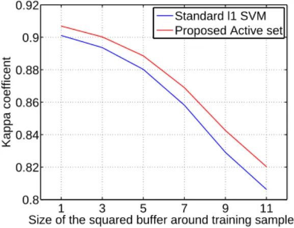
A last issue with the numerical assessment is related to the dependence between training and testing samples: in the setting discussed above, the test pixels are all the labeled pixels not contained in the training set. Therefore, and especially since we are using mostly spatial filters based on moving win-dows, the values of adjacent pixels can be highly correlated, which biases positively the results. To study this phenomenon, we eliminated from the test set pixels located in the spatial proximity of the training samples, by applying a buffer of increasing size around all the training samples. Figure 4 compares the performance of the proposed AS-Bands with the ALLℓ1linear SVM: the positive bias is clearly observed,
since the Kappa score decreases for buffers of increasing size. This is related both to the dependence between training and testing samples, but also to the fact that, for large buffers, almost the entirety of the test set is located at the borders of the labeled polygons in the ground reference; these areas are those with the highest degree of spectral mixing and are more complex to classify. However, the gain of the proposed system on the method using pre-defined filterbanks is constant, showing the consistency of the approach over the competing methods.
Features discovered. We now analyze the features extracted by the AS approach for one of the five runs performed (Fig. 5).
We remind the reader that the AS method can generate all
possible filters of the type described in Table III and thus scans the wide spaceΘ of the morphological, textural and attribute
TABLE III
FILTERS LIBRARY USED IN THE EXPERIMENTS,ALONG WITH THEIR PARAMETERS AND POSSIBLE VALUES
Bank Filters Parameters Type Search range
Br ¨uttisellen Indian Pines
All filters - Band (or PCA) int [1 : b]
Opening, Closing, Opening top-hat, - Shape of structuring element str {disk, diamond∗,
Closing top-hat, Opening by recon- square∗, line∗}
Morphological
struction, Closing by reconstruction, - Size of structuring element int [1 : 2 : 11] [1 : 2 : 21]
(MOR [16])
Opening by reconstruction top-hat and Closing by reconstruction top-hat
- Angle∗(if Shape = ‘line’) float [0, π]
Texture [4] Mean, Range, Entropy and Std. dev. - moving window size int [3 : 2 : 21]
Attribute Area - Area int [100 : 1000 : 10000]
(ATT [25]) Diagonal - Diagonal of bounding box int [10 : 10 : 100]
Inertia - Moment of inertia float [0.1 : 0.1 : 1] N/A
Standard deviation - Standard deviation float [0.5 : 5 : 50] N/A
∗used only in the AS experiment
TABLE IV
AVERAGED NUMERICAL FIGURES OF MERIT OF THE CONSIDERED STRATEGIES FOR THEBRUTTISELLEN DATASET¨ . RESULTS ARE COMPARED TOℓ1AND
ℓ2SVMS USING THE ORIGINAL BANDS(BA N D S,NO SPATIAL INFORMATION)AND CONTEXTUAL FILTERS GENERATED FROM THE3FIRSTPCS AND THE WHOLE SET OF POSSIBLE FEATURES INTABLEIII (THEALLSET CONTAINS ALL MORPHOLOGICAL,ATTRIBUTE AND TEXTURE FILTERS).
Pre-generated filterbanks library Active set
SVM Model ℓ1 ℓ◦2 ℓ2 ℓ1 ℓ+2
Feature set Bands MOR ATT ALL Bands MOR ATT ALL Bands MOR ATT ALL AS-Bands AS-Bands
Residential 76.71 87.60 92.44 88.75 77.78 90.93 91.76 92.15 76.50 93.65 92.64 94.24 96.71 95.89 Commercial 51.49 76.08 66.42 87.66 50.88 79.50 71.35 90.84 50.11 87.92 79.97 93.88 83.73 87.82 Meadows 99.93 87.76 99.58 97.63 99.80 96.13 99.18 99.25 99.80 98.83 99.43 99.64 99.60 99.37 Harvested 0 98.61 83.24 97.13 0.25 97.58 97.99 98.26 0.53 97.73 98.80 98.91 97.51 99.61 Bare soil 49.53 96.86 99.41 99.95 70.76 99.82 99.97 99.97 82.48 99.93 99.93 99.98 99.91 99.98 Roads 88.92 76.56 84.32 83.44 86.74 80.55 84.67 88.15 86.40 85.58 86.46 90.42 89.39 89.73 Pools 21.09 99.92 98.28 100.0 92.89 99.14 99.92 98.09 92.96 90.85 99.61 97.30 96.40 98.75 Parking 0 74.93 31.26 80.67 0 73.55 44.59 82.28 0 81.96 72.38 87.03 51.99 71.37 Trees 0 94.21 12.81 93.93 19.21 93.52 34.25 92.22 20.05 94.60 76.33 94.64 65.93 88.61 Overall accuracy 69.75 85.27 85.50 92.16 72.47 90.20 88.08 94.41 73.25 93.67 92.06 95.90 92.46 94.42 Cohen’s Kappa 0.613 0.816 0.819 0.903 0.650 0.879 0.852 0.931 0.660 0.922 0.902 0.950 0.907 0.931
# features per class 4 196 324 556 4 196 324 556 4 196 324 556 ∞
Active features (µ) 4 10 13 20 4 10 13 20 4 196 324 556 23
Is AS-Bands better? Yes Yes Yes Same Yes Yes Yes Same Yes Same Yes No – –
+= on features selected by the active set algorithm only
◦= on features selected by the l
1 SVM only 1 3 5 7 9 11 0.8 0.82 0.84 0.86 0.88 0.9 0.92
Size of the squared buffer around training samples
Kappa coefficent
Standard l1 SVM Proposed Active set
Fig. 4. Performance bias introduced by adjacency of training and testing
samples. Comparison between the ℓ1SVM (ALL feature set) and the proposed
AS-Bandsstrategy.
filters. As there are continuously parametrized filters (angular filters, attribute filters), the space of valid filter functions is infinitely dimensional. The first pie chart in Fig. 5(a) illustrates the proportion of filter types selected by the ℓ1 AS-Bands
Top hat 25% Attribute inertia 17% Attribute area 13% Opening / closing 12% Top-hat by reconstruction 9% Texture, std 6% Texture, entropy, 5% Attribute, diagonal 5% Texture, range 4% Reconstruction, 3% Other, 2% Residential (31) Commercial (50) Meadows (30) Harvested (21) Bare soil (7) Roads (49) Pools (5) Parkings (22) Trees (14) (a) (b)
Fig. 5. Infinite active set algorithm: (a) selected filterbank per type and (b)
number of retained features per class.
method. Morphological top hat, inertia and area attributes filters compose more the 55% of the discovered features. This is clearly related to the object characteristics: top-hat pro-vides important information about the contrast of the objects (depending on the scale, locally dark or bright objects are emphasized), while inertia is important for elongated objects (such as roads) and area for wide smooth classes (such as bare soil). Since the process is run independently for each class, the classification sub-problems can be analyzed in terms of selected variables. Since the proposed AS method extracts
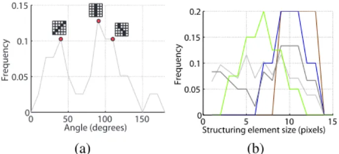
separate features for each class, it is possible to study the features that have been selected specifically for a given land use discrimination problem. Figure 5(b) depicts the number of active features for each OAA subproblem. This gives rough information about the spatial complexity of the classes, as strongly textured classes will require more spatial features to be discriminated. For instance, the class ‘commercial’ required 50 features to be optimally discriminated from the rest: by observing the spatial arrangement of this class, this choice results appropriate since the discrimination of commercial buildings with different spatial arrangements (parkings on roofs, for example) mainly rely on the geometrical properties of this class. Another spectrally ambiguous category are the ‘roads’. The separation of this class required the use of 49 features, again mainly composed by morphological top-hat and attribute inertia (the objects are mainly elongated). Even more interestingly, a large portion of the latter were directional filters, i.e. the structuring element was a line with a specific orientation. In particular, three main orientations arise, as illustrated in Fig. 6(a): these correspond to the main road directions in the image (three peaks in the angles). This observation can be coupled with the plot depicting the frequency of the chosen size of the structuring elements of the morphological operators for each class, in Fig. 6(b). By looking at the curve for the ‘road’ class, it appears that these three main directions are selected among a uniform range of possible sizes of the structuring element. It makes sense that longer structuring elements are oriented as the main road directions, while the shortest are acting inside the road, to filter arbitrarily oriented roads. Otherwise, for the other classes, the optimal size of the structuring elements is correlated to the size of the objects represented in the ground, for instance 7 pixels for trees, from 8 to 14 for bare soil and so on.
Summing up, the results illustrated that the proposed feature learning system selects automatically the variables optimizing class discrimination, since their selection is based on the maximization of the SVM margin. Note that these are not formally the best possible features, as we do not consider the entirety of the generable possible filtered images in the infinitely large filters space. Nonetheless, the features retained are those that optimized class separation among the large amount of features considered. We recall that the only in-formation provided to the system, is the type and family of the possible filters Θ, from Tab. III. As a result, extracted features related to characteristics directly observable on the ground cover are retained for classification, in a completely automatic way. In addition, since the selection is performed per class, the parameters of the transformations corrsponding to the selected features are directly related to the geometrical, textural or spectral characteristics of the objects belonging to that semantic class.
B. Hyperspectral image of Indiana
Numerical assessment. Table V presents the numerical accuracy for the Indian Pines 2010 dataset. Experiments are organized as for the previous case study, but the standard ℓ1
SVM has been run varying the value of the λ parameter: we
0 50 100 150 0 0.05 0.1 0.15 Angle (degrees) Frequency 0 5 10 15 0 0.05 0.1 0.15 0.2
Structuring element size (pixels)
Frequency
(a) (b)
Fig. 6. (a) Orientation of linear structuring elements for the class ‘roads’.
(b) Structuring element size within the morphological filters selected for five classes (for color legend, refer to Tab. IV).
report two cases, one obtained with a large λ (λ = 100), thus enforcing strong sparsity and a second one with a small λ (λ = 1), thus allowing more features in the model. For the baseline methods, the choice of the regularizer λ is driven by the need of compact vs accurate solution: at a first glance, the sparse model performs much worse than the one obtained reducing the λ parameter: it shows a similar level of sparsity as the proposed method (17 active features – 4% of the precomputed set – against 23 in the AS results and 105 of the model with a smaller λ), but with results lower than those obtained with a smaller λ (losses between 8% in ALL to 24% in Bands). As a first observation, we can conclude that a strongly sparseℓ1model produces heavy
decreases in performance because relevant informations have been discarded in the feature selection process.
Considering the proposed AS method, such decrease is not observed. The results are close to the best for theℓ1case (only
the ALL ℓ1 model outperforms it) and are the best for the ℓ2
case. The performances are aκ of 0.922 per an average of 23 active features per class in the AS-Bands case and of 0.960 per 22 active features per class in the AS-PCA respectively. In light of these results, we observe that the AS strategies keep the level of sparsity of theℓ1 model with a largeλ, but with
the numerical performance of theℓ1 model with smallλ. This
is very interesting, since the model built on the subset of an average of 22 features per class discovered by the AS-PCA is always at least significantly comparable (and the most often better) than the ones built with precomputed libraries going up to 429 variables. The only exception is the ALL experiment with the ℓ1 norm, which outperforms our method in the ℓ1
setting.
Finally, remind that the AS results are obtained without bounding the search range of the parameters in Θ: this lets the model explore several scale and, up to a sufficient number of iterations, ensures the coverage of a multitude of them. This avoids the risk of missing the relevant features, simply because the prior knowledge about scales was wrong and the good features weren’t present Θ: this risk is real, since, for example, the performance of the ℓ1 model with smallλ and
the MOR features drops from 97.64% to 92.06% if the range of sizes of structuring element is restricted to [1 : 2 : 11], instead of the[1 : 2 : 21] used for the experiments reported in Tab. IV.
perfor-TABLE V
RESULTS OF THE PROPOSED ACTIVE SET ALGORITHM USING ORIGINAL BANDS(AS-BA N D S)OR THE50FIRSTPCS(AS-PCA). RESULTS ARE COMPARED TOℓ1ANDℓ2SVMS USING THE ORIGINAL BANDS(BA N D S,NO SPATIAL INFORMATION),THE TEN FIRSTPCS(PCA,NO SPATIAL INFORMATION)AND CONTEXTUAL FILTERS GENERATED FROM THE3FIRSTPCS AND THE WHOLE SET OF POSSIBLE FEATURES INTABLEIII (THEALLSET CONTAINS ALL
MORPHOLOGICAL,ATTRIBUTE AND TEXTURE FILTERS). THE NUMBER OF ACTIVE FEATURES REPORTED IS THE AVERAGE PER CLASS.
SVM Input features Active features Overall Accuracy Cohen’s Kappa Is AS better ?
λ type Feature set # per class µ σ µ σ µ σ AS-Bands AS-PCA
Acti v e set ℓ1 AS-Bands * 23 3 93.57 2.74 0.922 0.033 – No AS-PCA * 22 2 96.72 1.98 0.960 0.024 Yes – ℓ+ 2 AS-Bands * 23 3 97.69 0.29 0.972 0.004 – No AS-PCA * 22 2 99.29 0.22 0.991 0.003 Yes – Pre-generated filterbank library Lar ge λ (sparse) ℓ1
Bands 360 22 4 65.85 1.71 0.606 0.018 Yes Yes
PCA(10 PCs) 10 7 1 78.70 0.30 0.747 0.003 Yes Yes
MOR(from 3 PCs) 267 13 1 94.48 0.28 0.933 0.003 Same Yes
ATT(from 3 PCs) 123 10 3 79.33 0.64 0.754 0.007 Yes Yes
ALL(from 3 PCs) 429 17 5 93.84 1.07 0.925 0.013 Same Yes
ℓ◦
2
Bands 360 22 4 80.76 1.02 0.771 0.012 Yes Yes
PCA(10 PCs) 10 7 1 85.04 1.18 0.821 0.014 Yes Yes
MOR(from 3 PCs) 267 13 1 95.71 0.54 0.948 0.007 Yes Yes
ATT(from 3 PCs) 123 10 3 85.77 0.55 0.828 0.007 Yes Yes
ALL(from 3 PCs) 429 17 5 97.53 0.73 0.970 0.009 Same Yes
Small
λ
ℓ1
Bands 360 200 11 89.15 0.53 0.869 0.006 Yes Yes
PCA(10 PCs) 10 9 1 89.03 0.61 0.868 0.007 Yes Yes
MOR(from 3 PCs) 267 76 9 97.64 0.90 0.971 0.011 No Same
ATT(from 3 PCs) 123 48 11 90.87 0.81 0.889 0.010 Yes Yes
ALL(from 3 PCs) 429 105 13 98.69 0.63 0.984 0.008 No No
ℓ◦
2
Bands 360 200 11 93.43 0.45 0.920 0.005 Yes Yes
PCA(10 PCs) 10 9 1 87.17 0.70 0.846 0.008 Yes Yes
MOR(from 3 PCs) 267 76 9 98.19 0.52 0.978 0.006 Same Yes
ATT(from 3 PCs) 123 48 11 92.39 0.67 0.907 0.008 Yes Yes
ALL(from 3 PCs) 429 105 13 98.88 0.42 0.986 0.005 No Same
ℓ2
Bands 360 360 0 94.23 0.54 0.930 0.006 Yes Yes
PCA(10 PCs) 10 10 0 87.24 0.72 0.846 0.008 Yes Yes
MOR(from 3 PCs) 267 267 0 98.18 0.58 0.978 0.007 Same Yes
ATT(from 3 PCs) 123 123 0 92.99 0.52 0.914 0.006 Yes Yes
ALL(from 3 PCs) 429 429 0 99.13 0.24 0.989 0.003 No Same
+= on features selected by the active set algorithm only
◦= on features selected by the ℓ
1 SVM only
mances of the AS-Bands and AS-PCA schemes, we detail some of the results by analyzing the retained active features. Recall that, as in the previous case study, no information about the feature is provided to the AS method beforehand: the features are discovered iteratively by the algorithm itself.
In each experiment, the retained features correspond to a specific filter (family, type and parameters) computed on a selected spectral band or on one of the first 50 PCs. In Fig. 7, the sampling frequency of a specific variable to be filtered (from either the original channels or the PCs) is illustrated for the average of the five runs reported in the numerical
0 100 200 300 0 2 4 6 8 10 Band index
Number of times selected (average)
0 10 20 30 40 50 0 5 10 15 20 PCAs index
Number of times selected (average)
(a) AS-Bands (b) AS-PCA
Fig. 7. Variables selected for filtering in one run of the (a) AS-Bands and
(b) AS-PCA experiments, respectively, for the Indian Pines dataset. The plots report the average of the bands selected by five runs of the algorithm with different initializations.
assessment. The single runs results are relatively consistent between each other, thus showing that, even if the selection of the bands to be filtered is random, the algorithm tends to select the same (or adjacent, thus highly correlated) channels. Two main observation can be made. When starting from the original image, feature composing the final set are not redundant one to each other. This is especially interesting, since we aim at compact models with few features. In Fig. 7(a), it appears that the retained group of bands are concentrated around
specific wavelengths far one from each other. Class-specific
histograms are reported in the second column of Fig. 8. The wavelengths selected are directly related with the class to be discriminated. Observing the plot in Fig. 7(b) and by following the aforementioned considerations, we can state that the first components of the PCA, corresponding to a high empirical variance, are not the only ones contributing to the discrimination. On the contrary, many featurescorresponding
to higher frequencies (lower variance) are retained, suggesting that very useful information is still present in the small-eigenvalue spectrum part of the PCA components,as observed
in previous literature [?], [?].
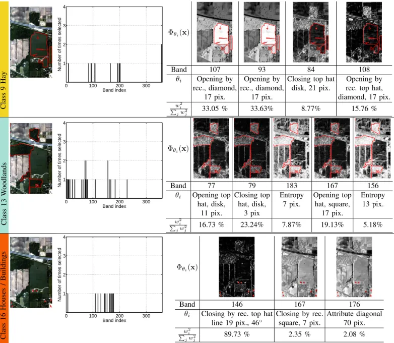
These interesting statements are further detailed in Fig. 8 and Fig. 9. In the former, examples of features retained for three different OAA subproblems are detailed. The class ‘Hay’ corresponds to large patches of dense vegetation. This specific class is outlined in red in the RGB image, as well
as to the retained filtered variables. By looking at the plot illustrating the frequency of selection of the bands along the 5 experiments, a preference on the spectral wavelength useful to discriminate this class did not appear. The filters applied to these spectral bands are in the form of smoothing operations, such as the opening by reconstruction (together take more than the 66% of the squared cumulative weights). Also, top-hat morphological operations are used (24.53% of the weights), particularly useful to reduce ambiguity with the other densely vegetated class, such as the ‘Woodlands’, which is detailed in the second row of the figure. This time, a series of top-hat morphological operations with different structuring elements and texture indicators (entropy) contribute in the squared cumulative weight scoring for the 72.15%. This time, the systems take advantage of the texture that characterize the forest. The last example for the AS-Bands is related to the ‘Houses / Buildings’ class. The highest feature weight has been assigned to a closing by reconstruction top-hat morphological filter, clearly emphasizing the locally dark behaviour of the buildings. However, note that this feature did not only discriminate houses, but also other small objects
characterized by similar structure / contrast. For this reason,
two other features are kept, in particular to discriminate
between houses and other similar structures. Note how, for the three classes, different spectral ranges are selected for the bands to be filtered.
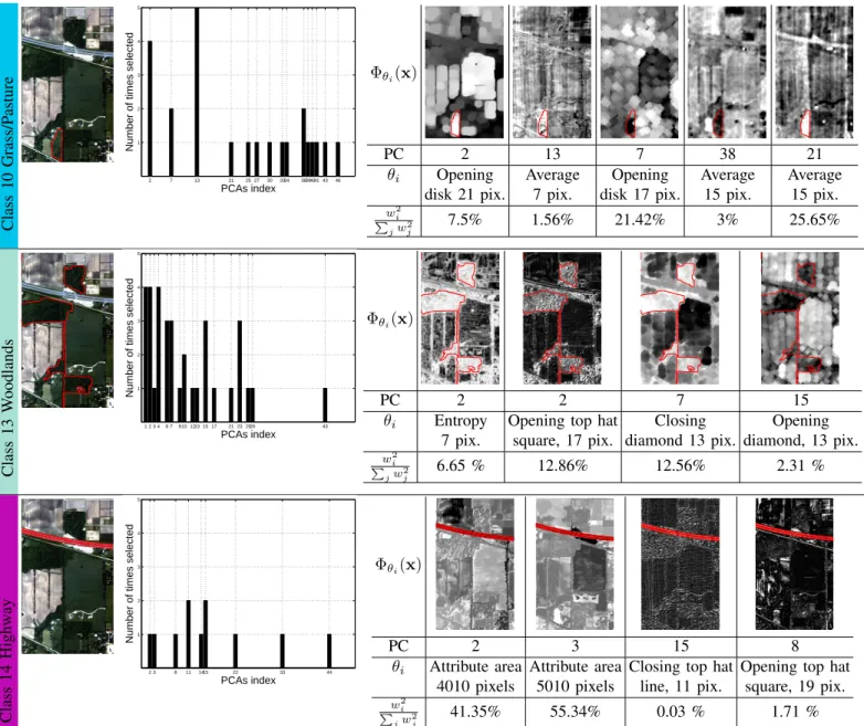
Figure 9 illustrates the retained features in the AS-PCA experiments. The first example provides insights for the dis-crimination of the ‘Grass/Pasture’ class. Interestingly, the 13th
principal component has been selected 5 times and the second PC 4 times. Observing in detail the features, the outlined class is clearly discriminated from similar regions, in particular by the moving average feature, computed on the 21st principal
component taking the 25.65% of the squared cumulative SVM weights. It is worth emphasizing that many principal components higher than the 21st are the base information for
the retained filters, suggesting again that higher frequencies / low variance components still carry discriminative information for the classification problem, rather than just noise, as it is usually admitted in remote sensing literature. By analyzing the next example, the ‘Woodlands’ class, it appears that features discriminating well this class are computed from the lower frequencies of the PCA. 3rd, are selected 4 times.
The last example is related to the discrimination of the class ‘Road’. This ground cover is spatially well structured, a fact that is reflected in the choice of the attribute area features computed over low frequency components. It results that the first two features, that sum to 96.69% for the squared weight contribution, easily discriminate the roads by assigning to them very low values. The remaining features, less important, filter out additional ambiguities related to this specific OAA problem.
Summing up, we observed that the AS feature learning scheme is able to discover spatial and contextual variables that optimize the classification problem. From both the accuracy and the visual points of view, these features appear consistent with both VHR and HS classification problems.
Is this better than random selection? In these last
exper-iments, we would like to compare the proposed AS scheme to a random inclusion of spatial filters. This would prove that the active set criterion of Eq. (5) is valid and, while providing a decrease of the SVM cost by definition, in our case, it also helps in improving the SVM global classification performance. To do so, we compared the active set feature selection-based approach with a random ‘sampling’ of the spatial filter, in which a randomly selected feature φθj is added at each
iteration to the active set ϕ, without checking whether it violates its optimality conditions. The ℓ1 SVM is retrained
after each iteration. This type of validation is standard when considering active learning methods [49], [50], which sample the most informative samples (contrarily to features here) among a large amount of unlabeled pixels.
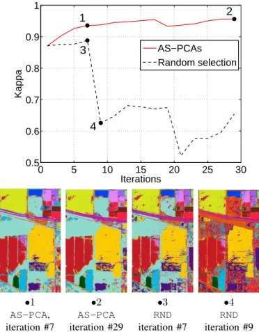
In Fig. 10 this process is illustrated in terms of estimatedκ statistic. The plot shows clearly that the AS-PCA constantly increases the classification accuracy by encoding a margin maximization strategy, while the random strategy is stable until the point, where a feature destroying the structure of a main class is added to the model. At this point, the classification accuracy drops. This is illustrated by classification maps generated from two points on each curve. Maps at points •1 and•2 show a clear increase in the map quality, while in this example•3 and •4 show a degradation in the map coherence. This process can be seen as an active learning of the optimal featurespace for classification, and the violating constraint as the contribution to the error reduction if the feature is included in the current active set.
V. CONCLUSIONS
We proposed an active set algorithm to discover the con-textual features that are important to solve a remote sensing image classification task. The algorithm screens randomly generated filterbanks, without any prior knowledge on the filter parameters (which are specific to the filter type, image contents and they are potentially continuous and thus related to an infinity of possible features). Based on a sparseℓ1linear SVM,
the algorithm evaluates if a feature would lead to a decrease in the SVM decision function if added to the current feature set.
Experiments on VHR multi- and hyperspectral images con-firmed the interest of the method, which is capable of retriev-ing for each class the most discriminant features in a large search space (possibly infinite for continuous parametrized filter types). Visual inspection of the retained features allows one to appreciate the class separability of the top ranked features.
Based on this subset, an ℓ2 SVM can also be trained,
leading to additional boosts in classification performance. In both cases (ℓ1 and ℓ2 SVMs), the models trained on the
features discovered reach comparable or better performance as SVM trained with predefined filterbanks defined by user prior knowledge. Moreover, the progression of the accuracy is almost monotonic, in contrast to inclusion of some randomly generated features, where a non-discriminative feature can lead to degradation of performances.
Future research will consider weighting of the bands (or pro-jections) to be filtered, in order to let the algorithm gradually
0 5 10 15 20 25 30 0.5 0.6 0.7 0.8 0.9 1
3
4
1
2
Iterations Kappa AS−PCAs Random selection •1 •2 •3 •4 AS-PCA, AS-PCA RND RNDiteration #7 iteration #29 iteration #7 iteration #9
Fig. 10. Top: comparison between the thirty first iterations of one run of
the AS-PCA algorithm and a random selection of the spatial filters. Bottom,
classification maps obtained at points[1, 2, 3, 4] on the respective curves.
ignore regions of the input space that lead to uninteresting spatial features not contributing to the model improvement. Such a weighting must be handled with care, since it may lead to trapping in local minima and consequent ignorance of relevant subspaces that contain discriminative features. Semi-supervised extensions will also be topics of interest, to enforce even more the desirable properties of the algorithm in extremely small sample scenarios.
ACKNOWLEDGEMENTS
The authors would like to acknowledge Prof. Mikhail Kanevski (CRET, Universit´e of Lausanne) for the access to the QB image “Br¨uttisellen” and The Laboratory for Appli-cations of Remote Sensing at Purdue University and the US Department of Agriculture, Agricultural Research Service, for the access to the “Indian Pines 2010” SpecTIR image.
REFERENCES
[1] M. Fauvel, J. Chanussot, and J.A. Benediktsson, “Decision fusion for the classification of urban remote sensing images,” IEEE Trans. Geosci. Remote Sens., vol. 44, no. 10, pp. 2828–2838, 2006.
[2] D. Tuia, F. Pacifici, M. Kanevski, and W.J. Emery, “Classification of very high spatial resolution imagery using mathematical morphology and support vector machines,” IEEE Trans. Geosci. Remote Sens., vol. 47, no. 11, pp. 3866–3879, 2009.
[3] A. Puissant, J. Hirsch, and C. Weber, “The utility of texture analysis to improve per-pixel classification for high to very high spatial resolution imagery,” Int. J. Remote Sens., vol. 26, no. 4, pp. 733–745, 2005.
[4] F. Pacifici, M. Chini, and W.J. Emery, “A neural network approach using multi-scale textural metrics from very high-resolution panchromatic imagery for urban land-use classification,” Remote Sens. Environ., vol. 113, no. 6, pp. 1276–1292, 2009.
[5] N. Longbotham, C. Chaapel, L. Bleiler, C. Padwick, W. J. Emery, and F. Pacifici, “Very high resolution multiangle urban classification analysis,” IEEE Trans. Geosci. Remote Sens., vol. 50, no. 4, pp. 1155– 1170, 2012.
[6] P. J. Pinter, J. L. Hatfield, J. S. Schepers, E. M. Barnes, S. Moran, C. S. T. Daughtry, and D. R. Upchurch, “Remote sensing for crop management,” Photogramm. Eng. Rem. S., vol. 69, no. 6, pp. 647–664, 2003. [7] D. Haboudane, N. Tremblay, J.R. Miller, and P. Vigneault, “Remote
estimation of crop chlorophyll content using spectral indices derived from hyperspectral data,” IEEE Trans. Geosci. Remote Sens., vol. 46, pp. 423–437, 2008.
[8] J.-B. F´eret and G. Asner, “Semi-supervised methods to identify
individual crowns of lowland tropical canopy species using imaging spectroscopy and LiDAR,” Remote Sens., vol. 4, pp. 2457–2476, 2012. [9] M.A. Cho, R. Mathieu, G.P. Asner, L. Naidoo, J. van Aardt, A. Ramoelo, P. Debba, K. Wessels, R. Main, I.P.J. Smith, and B. Erasmus, “Mapping tree species composition in sourth african savannas using an integrated airborne spectral and lidar system,” Remote Sens. of Environ., vol. 125, pp. 214–226, 2012.
[10] A. Plaza, J. A. Benediktsson, J. Boardman, J. Brazile, L. Bruzzone, G. Camps-Valls, J. Chanussot, M. Fauvel, P. Gamba, A. Gualtieri,
M. Marconcini, J.C. Tilton, and G. Trianni, “Recent advances in
techniques for hyperspectral image processing,” Remote Sens. Environ., vol. 113, no. Supplement 1, pp. S110–S122, 2009.
[11] J. Verrelst, M. E. Schaepmann, B. Koetz, and M. Kneub¨uhler, “Angular sensitivity analysis of vegetation indices derived from CHRIS/PROBA data,” Remote Sens. Enviro., vol. 112, pp. 2341–2353, 2008.
[12] S. Stagakis, N. Markos, O. Skyoti, and A. Kirparissis, “Monitoring canopy biophysical and biochemical parameters in ecosystem scale using satellite hyperspectral imagery: an application on a Phlomis fructicosa Mediterranean ecosystem using multisangular CHRIS/PROBA observa-tions,” Remote Sens. Enviro., vol. 114, pp. 977–994, 2010.
[13] M. Jehle, A. Hueni, A. Damm, P. D’Odorico, J. Weyermann, M. Kneubiihler, D. Schlapfer, M.E. Schaepman, and K. Meuleman, “Apex -current status, performance and validation concept,” in Sensors, 2010 IEEE, nov. 2010, pp. 533 –537.
[14] H. Saari, V. V. Aallos, C. Holmlund, J. M¨akynen, B. Delaur´e, K. Nack-aerts, and B. Michiels, “Novel hyperspectral imager for lightweight
uavs,” in SPIE Airborne Intelligence, Surveillance, Reconnaissance
(ISR) Systems and Applications, 2010, vol. 7668.
[15] M. Fauvel, Y. Tarabalka, J. A. Benediktsson, J. Chanussot, and J. C.
Tilton, “Advances in spectral-spatial classification of hyperspectral
images,” Proceedings of the IEEE, vol. PP, no. 99, pp. 1 –24, 2013. [16] J.A. Benediktsson, J. A. Palmason, and J. R. Sveinsson, “Classification
of hyperspectral data from urban areas based on extended morphological profiles,” IEEE Trans. Geosci. Remote Sens., vol. 43, no. 3, pp. 480–490, 2005.
[17] G. Licciardi, F. Pacifici, D. Tuia, S. Prasad, T. West, F. Giacco, J. Inglada, E. Christophe, J. Chanussot, and P. Gamba, “Decision fusion for the classification of hyperspectral data: Outcome of the 2008 GRS-S data fusion contest,” IEEE Trans. Geosci. Remote Sens., vol. 47, no. 11, pp. 3857–3865, 2009.
[18] A. Baraldi and F. Parmiggiani, “An investigation of the textural
characteristics associated with gray level cooccurrence matrix statistical parameters,” IEEE Trans. Geosci. Remote Sens., vol. 33, no. 2, pp. 293–304, 1995.
[19] C. A. Coburn and A.C.B. Roberts, “A multiscale texture analysis
procedure for improved forest and stand classification,” Int. J. Remote Sens., vol. 25, no. 20, pp. 4287–4308, 2004.
[20] M. Volpi, D. Tuia, F. Bovolo, M. Kanevski, and L. Bruzzone, “Super-vised change detection in VHR images using contextual information and support vector machines,” Int. J. Appl. Earth Obs. Geoinf., vol. 20, pp. 77–85, 2013.
[21] M. Pesaresi and I. Kannellopoulos, “Detection of urban features using morphological based segmentation and very high resolution remotely sensed data,” in Machine Vision and Advanced Image Processing in Remote Sensing, Kannelopoulos I., G.G. Wilkinson, and T. Moons, Eds. Springer Verlag, 1999.
[22] M. Pesaresi and J.A. Benediktsson, “A new approach for the morpho-logical segmentation of high-resolution satellite images,” IEEE Trans. Geosci. Remote Sens., vol. 39, no. 2, pp. 309–320, 2001.
applied to geoscience and remote sensing,” IEEE Trans. Geosci. Remote Sens., vol. 40, no. 9, pp. 2042–2055, 2002.
[24] D. Tuia, F. Ratle, A. Pozdnoukhov, and G. Camps-Valls, “Multi-source composite kernels for urban image classification,” IEEE Geosci. Remote Sens. Lett., Special Issue ESA EUSC, vol. 7, no. 1, pp. 88–92, 2010. [25] M. Dalla Mura, J. Atli Benediktsson, B. Waske, and L. Bruzzone,
“Morphological attribute profiles for the analysis of very high resolution images,” IEEE Trans. Geosci. Remote Sens., vol. 48, no. 10, pp. 3747– 3762, 2010.
[26] N. Longbotham, F. Pacifici, T. Glenn, A. Zare, M. Volpi, D. Tuia, E. Christophe, J. Michel, J. Inglada, J. Chanussot, and Q. Du, “Multi-modal change detection, application to the detection of flooded areas: outcome of the 2009-2010 data fusion contest,” IEEE J. Sel. Topics Appl. Earth Observ., vol. 5, no. 1, pp. 331–342, 2012.
[27] P. Kruizinga, N. Petkov, and S.E. Grigorescu, “Comparison of texture features based on gabor filters,” in Proceedings of Image Analysis and Processing, Venice, Italy, 1999, pp. 142–147.
[28] D.A. Clausi and H. Deng, “Design-based texture feature fusion using gabor filters and co-occurrence probabilities,” IEEE Trans. Im. Proc., vol. 14, no. 7, pp. 925–936, 2005.
[29] L.M. Bruce, C.H. Koger, and Jiang Li, “Dimensionality reduction of hyperspectral data using discrete wavelet transform feature extraction,” IEEE Trans. Geosc. Remote Sens., vol. 40, no. 10, pp. 2331 – 2338, 2002.
[30] S.K. Meher, B.U. Shankar, and A. Ghosh, “Wavelet-feature-based
classifiers for multispectral remote-sensing images,” IEEE Trans. Geosc. Remote Sens., vol. 45, no. 6, pp. 1881 –1886, 2007.
[31] S. Prasad, Wei Li, J.E. Fowler, and L.M. Bruce, “Information fusion in the redundant-wavelet-transform domain for noise-robust hyperspectral classification,” IEEE Trans. Geosci. Remote Sens., vol. 50, no. 9, pp. 3474–3486, 2012.
[32] Liangpei Zhang, Xin Huang, Bo Huang, and Pingxiang Li, “A pixel shape index coupled with spectral information for classification of high spatial resolution remotely sensed imagery,” IEEE Trans. Ge, vol. 44, no. 10, pp. 2950 –2961, 2006.
[33] X. Huang and L. Zhang, “Classification and extraction of spatial features
in urban areas using high-resolution multispectral imagery,” IEEE
Geosci. Remote Sens. Lett., vol. 4, no. 2, pp. 260–264, 2007. [34] L. Bruzzone and S.B. Serpico, “A technique for features selection in
multiclass problems,” Int. J. Remote Sens., vol. 21, no. 3, pp. 549–563, 2000.
[35] G. Camps-Valls, J. Mooij, and B. Scholkopf, “Remote sensing feature selection by kernel dependence measures,” IEEE Geosci. Remote Sens. Lett., vol. 7, no. 3, pp. 587 –591, 2010.
[36] B. Kuo and D. Landgrebe, “Nonparametric weighted feature extraction for classification,” IEEE Trans. Geosc. Remote Sens., vol. 42, no. 5, pp. 1096–1105, 2004.
[37] L. G´omez-Chova, R. Jenssen, and G. Camps-Valls, “Kernel entropy component analysis for remote sensing image clustering,” IEEE Geosci. Remote Sens. Lett., vol. 9, no. 2, pp. 312 –316, 2012.
[38] C.M. Bachman, T.L. Ainsworth, and R.A. Fusina, “Exploiting manifold geometry in hyperspectral imagery,” IEEE Trans. Geosci. Remote Sens., vol. 43, no. 3, pp. 441–454, 2005.
[39] P. R. Marpu, M. Pedergnana, M. Dalla Mura, S. Peeters, J. A.
Benedik-tsson, and L. Bruzzone, “Classification of hyperspectral data using
extended attribute profiles based on supervised and unsupervised feature extraction techniques,” International Journal of Image and Data Fusion, vol. 3, no. 3, pp. 269–298, 2012.
[40] G. Camps-Valls, L. G´omez-Chova, J. Mu–oz-Mar´ı, J. Vila-Franc´es, and J. Calpe-Maravilla, “Composite kernels for hyperspectral image classification,” IEEE Geosci. Remote Sens. Lett., vol. 3, no. 1, pp. 93– 97, 2006.
[41] D. Tuia, G. Camps-Valls, G. Matasci, and M. Kanevski, “Learning
relevant image features with multiple kernel classification,” IEEE Trans. Geosci. Remote Sens., vol. 48, no. 10, pp. 3780 – 3791, 2010. [42] M. Pedergnana, P. R. Marpu, M. Dalla Mura, J. A. Benediktsson, and
L. Bruzzone, “A novel technique for optimal feature selection in attribute
profiles based on genetic algorithms,” IEEE Trans. Geosci. Remote
Sens., in press.
[43] F. Bach, R. Jenatton, J. Mairal, and G. Obozinski, “Convex optimization with sparsity-inducing norms,” in Optimization for Machine Learning. MIT Press, 2011.
[44] S. Perkins, K. Lacker, and J. Theiler, “Grafting: Fast, incremental feature selection by gradient descent in function space,” J. Mach. Learn. Res., vol. 3, pp. 1333–1356, 2003.
[45] K. Glocer, D. Eads, and J. Theiler, “Online feature selection for pixel classification,” in Int. Conf. Machine Learn. ICML 05, Bonn (D)., 2005.
[46] N. R. Harvey, J. Theiler, S. P. Brumby, S. Perkins, J. J. Szymanski, J. J. BLoch, R. B. Porter, M. Galassi, and A. C. Young, “Comparison of GENIE and conventional supervised classifiers for multispectral image feature extraction,” IEEE Trans. Geosci. Remote Sens., vol. 40, no. 2, pp. 393–404, 2002.
[47] A. Rakotomamonjy, R. Flamary, and F. Yger, “Learning with infinitely many features,” Machine Learning, vol. 91, no. 1, pp. 43–66, 2013. [48] R. Flamary, F. Yger, and A. Rakotomamonjy, “Selecting from an infinite
set of features in SVM,” in European Symposium on Artificial Neural Networks ESANN, 2011.
[49] D. Tuia, M. Volpi, L. Copa, M. Kanevski, and J. Mu˜noz-Mar´ı, “A survey of active learning algorithms for supervised remote sensing image classification,” IEEE J. Sel. Topics Signal Proc., vol. 5, no. 3, pp. 606– 617, 2011.
[50] M. M. Crawford, D. Tuia, and L. H. Hyang, “Active learning: Any value for classification of remotely sensed data?,” Proceedings of the IEEE, vol. 101, no. 3, pp. 593–608, 2013.
Class 9 Hay 0 100 200 300 1 2 3 4 Band index
Number of times selected
Φθi(x)
Band 107 93 84 108
θi Opening by Opening by Closing top hat Opening by
rec., diamond, rec., diamond, disk, 21 pix. rec. top hat,
17 pix. 17 pix. diamond, 17 pix.
w2 i P jwj2 33.05 % 33.63% 8.77% 15.76 % Class 13 W oodlands 0 100 200 300 1 2 3 4 Band index
Number of times selected
Φθi(x)
Band 77 79 183 167 156
θi Opening top Closing top Entropy Opening top Entropy
hat, disk, hat, disk, 7 pix. hat, square, 13 pix.
11 pix. 3 pix 17 pix.
w2 i P jw2j 16.73 % 23.24% 7.87% 19.13% 5.18% Class 16 Houses / Buildings 0 100 200 300 1 2 3 4 Band index
Number of times selected
Φθi(x)
Band 146 167 176
θi Closing by rec. top hat Closing by rec. Attribute diagonal
line 19 pix., 46◦
square, 7 pix. 70 pix.
w2 i
P
jw2j 89.73 % 2.35 % 2.08 %